
Chapter 3
Stock Prices and Crude Oil Shocks: The Case of GCC Countries
F. Spagnolo*
Abstract
The aim of this chapter is to identify the effects of oil price volatility on stock market volatility for eight oil exporter or importer countries. Using weekly data for the 2004–15 period, we model the relationship between oil and stock prices using a multivariate GARCH–BEKK model. We find evidence of comovement between oil and stock markets, especially in the GCC region, whereas results for volatility spillovers are quite mixed. Consequently, general policies aimed at stabilizing stock prices in oil exporting countries cannot be formulated; the specific linkages between different markets need to be taken into account in order to devise appropriate policy measures.
Keywords
oil prices
VAR–GARCH model
volatility spillover
GCC Stock
JEL Classification
C32
F36
G15
1. Introduction
The relationship between oil and stock prices has been analyzed extensively in the recent literature. This chapter aims to shed light on the volatility spillover dynamics running from the oil market into stock market volatility for eight selected Middle Eastern/African frontier markets.a The methodology adopted in this chapter is based on the VAR–GARCH (vector autoregression–generalized autoregressive conditional heteroscedasticity) approach of Engle and Kroner (1995), which allows us to test for the presence of volatility spillover in both directions (ie, from oil prices to stock prices as well as in the opposite direction).
The effect of crude oil prices on US financial and economic variables is well documented in the literature. Hamilton (1996) uses an impulse response approach to show that US recessions were triggered by increases in oil prices. Ghouri (2006), using a linear model, finds that West Texas Intermediate (WTI) oil prices are inversely related to monthly US stock market returns.
Hammoudeh et al. (2004), using a GARCH methodology, find little evidence of spillover effects from oil prices to US stock prices. Elyasiani et al. (2012) compare specific industry sectors in the US stock market and find that, at industry level, there is strong evidence that global oil price volatility constitutes an asset price risk factor for most indices. Mollick and Assefa (2013) investigate the effect of oil on Standard & Poor’s (S&P) 500, Dow Jones, Nasdaq, and Russell 2000 index returns. The authors, also using a GARCH approach, show that US stock returns and WTI oil returns were, to some extent, negatively affected by both the oil prices and the exchange rate prior to the 2007 financial crisis. Moreover, their findings show that, after the onset of the financial crisis, stock returns were positively affected by oil prices and less affected by the exchange rate.
Nazlioglu et al. (2015) use an impulse response function methodology to examine the relationship between WTI and financial stress indices. The analysis, conducted by dividing the sample into a pre-2008 and a post-2008 crisis, shows evidence of significant spillovers in mean as well as in variance. Another recent study, by Salisu and Oloko (2015), considers a VARMA–BEKK–AGARCH (vector autoregressive moving average—Baba–Engle–Kraft–Kroner—asymmetric GARCH) approach to show that stock prices in the United States were more strongly affected by oil prices in the postcrisis period than they had been in the precrisis period.
Huang et al. (1996) use a vector autoregression (VAR) framework to investigate the causality between oil future prices and US stock prices and find weak evidence in terms of return volatility spillover for the period 1979–83. Using a similar approach, Kilian and Park (2009) investigate the relationship between oil and stock prices in the United States by looking at US oil refiners’ acquisition costs to find that US stock prices react differently depending on whether shocks are driven by demand or by supply, while Kang et al. (2014) replace stock prices with bond prices to find that demand and supply shocks originating from oil prices account for strong variations in the US bond market.
Balcilar and Ozdemir (2013) find evidence of nonlinearity between stock prices and oil prices and use a Markov switching model to argue that oil future prices might be a reliable predictor of the S&P 500 index. Alsalman and Herrera (2013), by means of the simultaneous equation method, find that an increase in the price of oil has an effect on UK stock indices up to 1 year ahead. Conrad et al. (2014) consider a modified dynamic conditional correlations–mixed data sampling (DCC–MIDAS) and find a positive oil–stock correlation during recessions and a negative one during economic expansions.
Park and Ratti (2008) and Apergis and Miller (2009) study several developed countries and find that the stock market is affected by positive oil shocks only in Norway (an oil exporter country). Arouri et al. (2011a) use a multifactor asset pricing model for 12 weekly European industrial sector indices and report evidence of substantial returns and volatility spillovers between oil and stock market prices. Arouri et al. (2011b) use a VAR–GARCH(1,1) model to test the relationship between daily oil and stock prices within the Gulf Cooperation Council (GCC) region, and show that oil prices tend to affect positively several stock markets in the region, while the volatility from GCC stock markets to oil markets is nearly absent. Jouini (2013) models weekly stock returns in Saudi Arabia from 2007 until 2011 by means of a VAR–GARCH model; results show evidence of significant and bidirectional spillovers between the Saudi Market Index and oil prices. Jouini and Harrathi (2014) consider a BEKK–GARCH model to revisit the empirical evidence regarding the volatility interactions among GCC stock markets and oil prices for the period 2005–11. Their findings suggest volatility spillover running from stock price volatility into oil market volatilities and vice versa. Zarour (2006) uses a VAR process to show that, while all GCC stock markets are affected by oil price shocks, Saudi and Omani stock market returns also affect oil prices. Lescaroux and Mignon (2008) examine the short- and long-run relationships between WTI oil prices and macroeconomic and financial indicators for oil exporting (including the GCC) and oil importing countries based on causality tests, cross-correlations, and cointegration techniques. Their analysis indicates that there exists a strong Granger causality running from oil to share prices, especially for oil exporting countries. Furthermore, oil prices were found to lead (countercyclically) share prices for the majority of the investigated countries.
Using a BEKK–GARCH model, Malik and Hammoudeh (2007) find that there is a significant volatility spillover running from oil to stock markets in the United States and GCC countries. Filis et al. (2011) compared three oil importing countries (Germany, the Netherlands, and the United States) and three oil exporting countries (Brazil, Canada, and Mexico) using a DCC–GARCH framework. Their results suggest that the relationship between oil and stock prices depends on the nature of the shocks; that is, demand shocks caused by drastic events, such as war, might affect stock markets more significantly than supply-side shocks originated by production cuts. The authors also find a correlation between lagged oil prices and stock market returns. Finally, Wang et al. (2013) use a structural VAR (SVAR) model to examine both oil importing countries (China, France, Germany, India, Italy, Japan, South Korea, the United Kingdom, and the United States) and oil exporting countries (Canada, Saudi Arabia, Kuwait, Mexico, Norway, Russia, and Venezuela). Their findings indicate that oil supply uncertainty can depress the stock markets of both oil exporter and importer countries.
2. The Model
We model the joint process governing oil and stock prices using a bivariate VAR–GARCH(1,1) framework.b The model has the following specification:
where xt = (stockt, oilt). The parameter vectors of the mean Eq. 3.1 are the constant α = (α1,α2) and the autoregressive term β = (β11, 0 | 0,β22). The residual vector ut = (e1,t,e2,t) is bivariate and normally distributed, ut | It − 1 ∼ (0, Ht), with a corresponding, conditional variance–covariance matrix given by

 (3.2)
(3.2)where

Eq. 3.3 models the dynamic process of Ht as a linear function of its own past values Ht − 1 and the past values of the squared innovations  . The BEKK model guarantees, by construction, that the covariance matrix in the system is positive definite. Given a sample of T observations, a vector of unknown parameters θ, and a 2 × 1 vector of variables xt, the conditional density function for the model, Eq. 3.1, is:
 (3.3)
(3.3)The log-likelihood function is:
 (3.4)
(3.4)Standard errors are calculated using the quasi-maximum likelihood method of Bollerslev and Wooldridge (1992), which is robust to the distribution of the underlying residuals.
3. Empirical Analysis
3.1. Data and Hypotheses Tested
We use weekly data for four GCC stock markets [the Kingdom of Saudi Arabia (KSA), Oman, Qatar, and the United Arab Emirates (UAE)], three frontier stock markets (Algeria, Morocco, and Namibia), as well as the United States for the period 6/1/2004 to 6/25/2015, for a total of 544 observations. WTI oil prices and stock prices were sourced by the US Energy Information Administration and Bloomberg, respectively. Weekly indices, Wednesday to Wednesday, were preferred in order to overcome the varying trading day closures of the different stock markets across the eight countries considered in this study. We define weekly returns as logarithmic differences of oil and stock prices. Descriptive statistics are reported in Table 3.1, along with plots of the data in Figs. 3.1 and 3.2. Namibia appears to be the most volatile stock market (out of the eight considered) with a standard deviation equal to 0.014, while Oman is the least volatile stock market with a standard deviation of 0.004. Oil prices show high volatility, with a standard deviation equal to 0.013.
Table 3.1
Descriptive Statistics
| Oil | KSA | UAE | Qatar | Oman | Algeria | Namibia | Morocco | USA | |
| Mean | 0.001 | 0.001 | 0.001 | 0.001 | 0.001 | 0.001 | 0.001 | 0.001 | 0.001 |
| Median | 0.001 | 0.001 | 0.001 | 0.001 | 0.001 | 0.001 | 0.001 | 0.001 | 0.001 |
| Maximum | 0.067 | 0.028 | 0.039 | 0.044 | 0.022 | 0.034 | 0.187 | 0.018 | 0.030 |
| Minimum | −0.076 | −0.103 | −0.075 | −0.059 | −0.054 | −0.041 | −0.175 | −0.035 | −0.042 |
| Std. dev. | 0.013 | 0.010 | 0.010 | 0.009 | 0.006 | 0.004 | 0.014 | 0.006 | 0.006 |
| Skewness | −0.465 | −3.168 | −1.138 | −0.883 | −2.541 | −2.314 | 0.631 | −0.972 | −0.923 |
| Kurtosis | 8.021 | 28.492 | 9.252 | 10.273 | 19.758 | 34.436 | 111.524 | 8.357 | 11.182 |
| Jarque–Bera | 620.4 | 1641.3 | 1053.3 | 1332.5 | 7296.3 | 2385.0 | 2280.7 | 767.2 | 1662.0 |
| Probability | 0.001 | 0.001 | 0.001 | 0.001 | 0.001 | 0.001 | 0.001 | 0.001 | 0.001 |
| Sum | 0.252 | −0.160 | −0.225 | 0.070 | −0.055 | 0.221 | 0.388 | 0.069 | 0.077 |
| Sum sq. dev. | 0.089 | 0.054 | 0.062 | 0.042 | 0.024 | 0.011 | 0.105 | 0.018 | 0.022 |

Note: Descriptive statistics on weekly data over the period 6/9/2004 to 6/10/2015.

Figure 3.1 Oil and GCC stock market returns.

Figure 3.2 Non-GCC stock market returns.
Following Caporale and Spagnolo (2003) and Al-Maadid et al. (2015), we use a multivariate GARCH–BEKK model to test for volatility spillover by placing restrictions on the relevant parameters. We consider the following two null hypotheses: (1) tests of no stock price volatility spillover to oil price volatility (H0: Stock → Oil: a21 = g21 = 0) and (2) tests of no oil price volatility spillover to stock price volatility (H0: Stock → Oil: a21 = g21 = 0).
3.2. Discussion of the Results
To test the adequacy of the models, Ljung–Box portmanteau tests were performed on the standardized and standardized squared residuals. Overall, the results indicate that the VAR–GARCH(1,1) specification satisfactorily captures the persistence in the returns and squared returns of all the series considered (Tables 3.2 and 3.3). Crossmarket dependence in the conditional variance varies in magnitude and direction across pairwise estimations.c The estimated VAR–GARCH(1,1) model with associated robust standard errors and likelihood function values is presented in Tables 3.2 and 3.3.
Table 3.2
Estimated VAR–GARCH(1,1) Model, GCC Countries
| KSA ≥ oil | UAE ≥ oil | Oil ≥ KSA | Oil ≥ UAE | ||||||
| Conditional mean | |||||||||
| Coef. | p-value | Coef. | p-value | Coef. | p-value | Coef. | p-value | ||
| α1 | 0.080 | (0.001) | 0.021 | (0.495) | α2 | 0.076 | (0.050) | 0.053 | (0.158) |
| β11 | 0.027 | (0.540) | 0.142 | (0.001) | β22 | −0.050 | (0.245) | −0.010 | (0.801) |
| Conditional variance | |||||||||
| C11 | 0.235 | (0.001) | 0.450 | (0.001) | C22 | 0.247 | (0.003) | 0.263 | (0.001) |
| C21 | −0.035 | (0.811) | −0.139 | (0.103) | |||||
| a11 | 0.639 | (0.001) | 0.453 | (0.001) | a22 | 0.276 | (0.001) | 0.345 | (0.001) |
| a21 | −0.055 | (0.230) | 0.103 | (0.034) | a12 | 0.017 | (0.829) | −0.038 | (0.536) |
| g11 | 0.753 | (0.001) | 0.754 | (0.001) | g22 | 0.933 | (0.001) | 0.884 | (0.001) |
| g21 | 0.012 | (0.776) | −0.010 | (0.722) | g12 | 0.051 | (0.421) | 0.130 | (0.090) |
| Log-lik. | −1424.658 | −1595.544 | |||||||
| Qstock(10) | 12.724 | (0.235) | 13.084 | (0.219) | AIC | 5.027 | 5.622 | ||
| Qoil(10) | 8.642 | (0.566) | 14.378 | (0.156) | HQ | 5.080 | 5.675 | ||
|
|
15.301 | (0.122) | 4.211 | (0.973) | SBC | 5.032 | 5.759 | ||
|
|
9.561 | (0.479) | 5.246 | (0.874) | |||||
| Qatar ≥ oil | Oman ≥ oil | Oil ≥ Qatar | Oil ≥ Oman | ||||||
| Conditional mean | |||||||||
| Coef. | p-value | Coef. | p-value | Coef. | p-value | Coef. | p-value | ||
| α11 | 0.035 | (0.042) | 0.026 | (0.064) | α22 | 0.062 | (0.120) | 0.051 | (0.191) |
| β11 | 0.114 | (0.004) | 0.145 | (0.000) | β22 | 0.063 | (0.225) | −0.043 | (0.232) |
| Conditional variance | |||||||||
| c11 | 0.168 | (0.000) | 0.216 | (0.000) | C22 | 0.268 | (0.000) | 0.156 | 0.000 |
| c21 | −0.012 | (0.853) | −0.042 | (0.701) | |||||
| a11 | 0.640 | (0.000) | 0.565 | (0.000) | a22 | 0.329 | (0.000) | 0.318 | (0.000) |
| a21 | 0.024 | (0.289) | −0.112 | (0.001) | a12 | −0.169 | (0.00) | −0.153 | (0.239) |
| g11 | 0.785 | (0.000) | 0.703 | (0.000) | g22 | 0.902 | (0.000) | 0.942 | (0.000) |
| g21 | −0.007 | (0.598) | 0.012 | (0.645) | g12 | 0.134 | (0.007) | 0.259 | (0.009) |
| Log-lik. | −1013.974 | −1208.977 | |||||||
| Qstock(10) | 9.618 | (0.477) | 13.958 | (0.175) | AIC | 4.895 | 4.283 | ||
| Qoil(10) | 14.534 | (0.150) | 14.606 | (0.147) | HQ | 3.655 | 4.336 | ||
|
|
7.000 | (0.726) | 6.3577 | (0.784) | SBC | 5.032 | 4.336 | ||
|
|
6.237 | (0.795) | 10.365 | (0.409) | |||||

Note: Standard errors (S.E.) are calculated using the quasi-maximum likelihood method of Bollerslev and Wooldridge (1992), which is robust to the distribution of the underlying residuals. Q(10) and ![]() are the Ljung–Box test (1978) of significance of autocorrelations of 10 lags in the standardized and standardized squared residuals, respectively. Parameter a12 measures the causality in variance effect of oil price volatility toward stock returns volatility. The covariance stationary condition is satisfied by all the estimated models. Note that in the conditional variance equation, the sign of the parameters is not relevant. Numbers are rounded to the third decimal.
are the Ljung–Box test (1978) of significance of autocorrelations of 10 lags in the standardized and standardized squared residuals, respectively. Parameter a12 measures the causality in variance effect of oil price volatility toward stock returns volatility. The covariance stationary condition is satisfied by all the estimated models. Note that in the conditional variance equation, the sign of the parameters is not relevant. Numbers are rounded to the third decimal.
Table 3.3
Estimated VAR–GARCH(1,1) Model, Non-GCC Countries
| Algeria ≥ oil | Namibia ≥ oil | Oil ≥ Algeria | Oil ≥ Namibia | ||||||
| Conditional mean | |||||||||
| Coef. | p-value | Coef. | p-value | Coef. | p-value | Coef. | p-value | ||
| α1 | 0.041 | (0.001) | 0.016 | (0.317) | α2 | 0.068 | (0.106) | 0.072 | (0.067) |
| β11 | 0.150 | (0.001) | −0.032 | (0.454) | β22 | −0.119 | (0.220) | −0.037 | (0.629) |
| Conditional variance | |||||||||
| C11 | 0.186 | (0.001) | 0.110 | (0.001) | C22 | 0.241 | (0.001) | 0.251 | (0.000) |
| C21 | 0.142 | (0.023) | −0.105 | (0.159) | |||||
| a11 | 0.358 | (0.001) | 0.299 | (0.001) | a21 | −0.003 | (0.672) | 0.017 | (0.422) |
| a12 | 0.141 | (0.248) | −0.085 | (0.433) | a22 | 0.376 | (0.001) | 0.359 | (0.001) |
| g11 | 0.749 | (0.001) | 0.929 | (0.001) | g22 | 0.908 | (0.001) | 0.915 | (0.001) |
| g21 | −0.252 | (0.103) | 0.002 | (0.871) | g12 | −0.251 | (0.103) | 0.038 | (0.447) |
| Log-lik. | −1424.658 | −1277.908 | |||||||
| Qstock(10) | 8.665 | (0.564) | 9.951 | (0.445) | AIC | 3.602 | 4.241 | ||
| Qoil(10) | 12.658 | (0.243) | 13.858 | (0.180) | HQ | 3.602 | 4.394 | ||
|
|
0.660 | (1.000) | 6.815 | (0.742) | SBC | 3.739 | 4.478 | ||
|
|
4.460 | (0.924) | 8.786 | (0.553) | |||||
| Morocco ≥ oil | USA ≥ oil | Oil ≥ Morocco | Oil ≥ USA | ||||||
| Conditional mean | |||||||||
| Coef. | p-value | Coef. | p-value | Coef. | p-value | Coef. | p-value | ||
| α1 | 0.103 | (0.001) | 0.016 | (0.317) | α2 | 0.063 | (0.093) | 0.072 | (0.067) |
| β11 | −0.039 | (0.359) | −0.032 | (0.455) | β22 | 0.020 | (0.545) | −0.037 | (0.629) |
| Conditional variance | |||||||||
| C11 | 0.344 | (0.001) | 0.110 | (0.001) | C22 | 0.255 | (0.001) | 0.251 | (0.001) |
| C21 | −0.027 | (0.691) | −0.105 | (0.159) | |||||
| a11 | 0.532 | (0.001) | 0.299 | (0.001) | a22 | 0.311 | (0.001) | 0.359 | (0.001) |
| a21 | 0.026 | (0.493) | 0.017 | (0.442) | a12 | −0.018 | (0.033) | −0.085 | (0.433) |
| g11 | 0.759 | (0.001) | 0.929 | (0.001) | g22 | 0.920 | (0.001) | 0.915 | (0.001) |
| g21 | −0.012 | (0.027) | 0.002 | (0.872) | g12 | 0.077 | (0.005) | 0.038 | (0.447) |
| Log-lik. | −1227.91 | −1206.651 | |||||||
| Qstock(10) | 3.450 | (0.969) | 7.405 | (0.687) | AIC | 5.315 | 4.267 | ||
| Qoil(10) | 14.874 | (0.137) | 15.192 | (0.125) | HQ | 5.368 | 4.320 | ||
|
|
0.062 | (1.000) | 8.784 | (0.553) | SBC | 5.451 | 4.404 | ||
|
|
11.308 | (0.334) | 7.490 | (0.679) | |||||

Notes: see notes in Table 3.2.
We select the optimal lag length of the mean equation using the Schwarz information criterion. The parameter estimates for the conditional variance equations show that the estimated “own market” coefficients are statistically significant for all stock markets with the estimates for g11, suggesting a high degree of persistence. Results can be summarized as follows:
• Volatility spillover from oil prices volatility into stock market returns volatility. The findings show a significant volatility shock spillover, measured by α12, running from oil prices into stock market prices in the cases of Morocco and Qatar, the greatest being for Qatar (0.169) and the least being for Morocco with a12 = 0.018. There is evidence of significant conditional volatility spillover, measured by g12, running from oil toward UAE (0.130), Qatar (0.134), and Oman (0.259). These results are consistent with findings reported in Arouri et al. (2011b), which show significant volatility spillovers between oil and stock markets in the GCC region.
• Volatility spillover from stock market returns volatility into oil prices volatility. There is significant volatility spillover running from stock market returns into oil prices only in the cases of UAE (a21 = 0.103) and Morocco (a21 = 0.012). These results are in line with the findings of Jouini (2013), showing that for the majority of the countries considered, shocks originating in the stock markets do not affect the oil prices volatility.
Conditional correlations, reported in Figs. 3.3 and 3.4, capture the comovements across oil prices and stock markets. They clearly show a higher (and positive) degree of comovement in the case of GCC countries compared to the other countries under investigation.
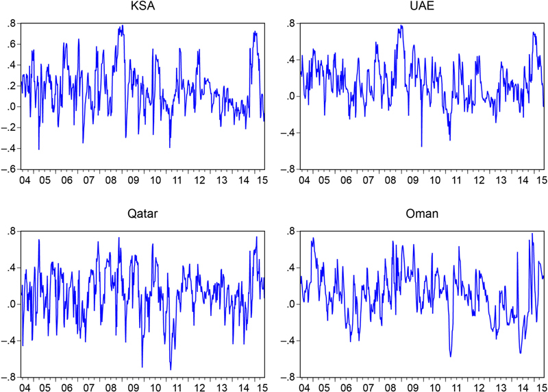
Figure 3.3 Conditional correlations between oil prices and GCC stock markets.

Figure 3.4 Conditional correlations between oil prices and non-GCC stock markets.
Overall, our results are in line with those from previous studies and suggest strong comovement between oil and stock markets, in particular for GCC countries. As far as volatility spillover is concerned, despite being relatively mixed, the results also show that oil price volatility can be seen as an important determinant of stock price volatility, specially in the GCC, as those countries are clearly more exposed to oil price shocks.
4. Conclusions
This chapter has investigated volatility spillovers between oil prices and stock market prices for eight countries selected by estimating a VAR–GARCH model with a BEKK representation. We have provided empirical evidence on the level of interdependence and volatility transmission between oil prices and several oil exporter stock market indices. Our findings have confirmed that stock markets and oil prices are highly and positively correlated. We have also found evidence of comovement between oil and stock markets, especially in the GCC region, whereas results for volatility spillovers are quite mixed. Consequently, general policies aimed at stabilizing stock price volatility in oil exporting countries cannot be formulated; the specific linkages between different markets need to be taken into account in order to devise appropriate policy measures.
..................Content has been hidden....................
You can't read the all page of ebook, please click here login for view all page.