Search in book...
Toggle Font Controls
Create new playlist

Name your new playlist

Playlist description (optional)
Sign In

Email address

Password

Forgot Password?

or

Continue with Facebook

Continue with Google
Sign Up

Full Name

Email address

Confirm Email Address

Password

or

Continue with Facebook

Continue with Google

Chapter 13

Frontier Market Investing: What’s the Value Add?

E.L. Black^*

S. Nogare^**
^* Cascade Cash Management, Newcastle Upon Tyne, United Kingdom
^** Accenture, New York City, NY, United States

Abstract

We propose that this chapter will assess the value of frontier markets from an investment perspective. The work we have already completed using a regime switching model in this area will be utilized, showing evidence that the value add of frontier markets is to improve the level of risk-adjusted returns while the extreme correlation of frontier markets in both bear and bull markets also has a positive effect on the overall investment. The growth projections of frontier markets, coupled with the lowering of international regulatory and liquidity constraints, suggest this is an area required for consideration in a client portfolio. We are happy to provide the work that we have already completed in this area as a contribution to the book.

Keywords

extreme correlation

portfolio exposure

frontier markets development

international diversification

regime switching model

1. Introduction

Stagnancy in developed nations has led investors to seek growth elsewhere. In the early 2000s, emerging markets occupied this space. The original BRIC economies of Brazil, Russia, India, and China provided above-average returns for the decade as respective governments established infrastructure and investment programs to fuel development. China sat as the central figure of the BRICs story, delivering double-digit growth as the People’s Republic industrialized rapidly, using the proceeds in an international shopping spree acquiring Western brands such as Volvo’s car division and IBM’s PC business. Brazil enjoyed Chinese demand for commodities, and Russia has established close oil links with China in a new geopolitical Beijing–Moscow trade axis. But is the Chinese story over? Growth has slowed, which has had ramifications for other emerging markets and raised volatility. As a result, investors and fund managers have looked to new frontiers in the quest for greater returns. The so-called MINT economies (Mexico, Indonesia, Nigeria, Turkey), as coined by Fidelity Investments, reflect expanding countries with rapidly growing populations and a young age demographic. The Financial Times Stock Exchange (FTSE) defines frontier markets as representing developing countries with high rates of economic growth, but small and relatively illiquid stock markets. This chapter considers the investment opportunity that frontier markets represent using a mean-variance and regime switching framework to evaluate their usefulness in investor and fund portfolios.

The increased correlation of international markets since the 2008 global financial crisis has profoundly affected the structure of modern investments. Globalization and financial market integration have grown exponentially since the 1980s. While capital market restrictions in the early years led to segmented global capital markets, since 2000 many foreign policies have become somewhat relaxed. Transnational corporations have provided jobs and local investment, but this has inadvertently meant that one country’s economic and fiscal difficulties can now easily filter into another, invoking contagion. Some growing economies, however, still suffer from poor corporate governance and large market illiquidity. Investors and fund managers have quickly adapted and financial innovation has spiked, with exchange-traded funds (ETFs) primarily offering passive access to these illiquid markets.

Countries rapidly develop by becoming part of the globalized world. Globalization and financial market integration have increased each country’s international exposure, producing tighter connections among national markets and adding complexity to modern portfolio management. The interconnectedness of global markets mostly relies on the intricate mechanisms within the overseas investments undertaken that have been driven by financial institutional investment and governmental policy.

This positive development of nations has been mostly connected with greater reward. Frontier markets have been cited as one of the leading classes with regard to upcoming development and infrastructural opportunities. Accordingly, international financial institutions have shown an increasing interest in these markets, allocating vast funds while creating new vehicles for investment exposure. In particular, attention has been placed around the governmental responsibility to adopt policies effectively that will permit reliable and consistent future growth. We believe that the ability and consistency to accomplish these tasks will determine the future path of each nation and, in turn, the level of investment profitability.

This chapter empirically begins by evaluating whether international opportunities in new upcoming markets exist by mainly understanding what frontier markets are and what they can truly offer. Moreover, due to the “nonnormality of returns,” “asymmetric correlation,” and “business cycles” requiring consideration in the process of portfolio asset allocation, we conduct deeper analysis, investigating periods of extreme correlation in an attempt to increase the evidence on countries’ international conduct under major worldwide shocks such as the Lehman Brothers collapse of 2008 or the European sovereign debt crisis, endured since mid-2010.

Additionally, in an attempt to better define the actual portfolio exposure in frontier markets, we then progress to investigate the effects of Markowitz’s (1952) strong assumption of the normal distribution of returns and the inability of using such an assumption in interpreting different economic states. We evaluate whether the probabilistic regime switching methodology (RSM) applied to real economic data remains flexible enough to produce a better asset allocation than Markowitz’s (1952) modern portfolio theory. In other words, we provide an answer as to the applicability of RSM in assessing both the investment opportunity and the danger presented by frontier markets.

The methodology utilized goes beyond the central concept that links Markowitz asset allocation to passive management. In 1990 the Compass Institute attempted to define the major problems regarding traditional asset allocation. The research determined that more attention to maximizing returns in up markets while protecting the investment in down markets was needed to create a consistent and reliable portfolio. The redefined approach was called adaptive asset allocation (AAA). With this evidence, the methodology involved attempts to exploit the possibility of a more dynamic process, concentrating on particular asset allocation methods which incorporate the probabilities and form each business cycle in the market. Thus, contrary to the traditional rebalancing method, market frequency and structure of past shocks play significant roles. However, in the process, attention to investors’ needs and the integrity of the portfolio structure does not have to be undermined.

The RSM generates superior portfolio performance when compared to Markowitz (1952). This is due to the ability of the model to account for a probabilistic analysis of the business cycle of each time series involved in the process. In addition, with the inclusion of the MSCI Frontier Markets Index of equities we find a further profit surge by opening the portfolio to notable international opportunities.

International investment is a regular component of most asset allocations due to the numerous and different advantages that each country or economic area presents. In fact, an international basket of assets is also able to offer a notable portfolio diversification, especially when country-specific risk is involved and managed. The Wealth Management Association (WMA; formerly APCIMS) guidelines suggest international allocations for overseas equity of 11% in even its conservative investment allocation. Frontier markets, due to their low correlation with the developed world, offer an attractive diversifying feature for investors willing to be subject to the inherent liquidity risk involved. Such risk can be mitigated through exposure indirectly via ETFs, for example.

To summarize, our findings indicate that frontier markets are evolving and provide an attractive outlet for investment. Opportunities are present, and diversification is achievable without a major problem of liquidity pressure. Furthermore, in most of the results frontier markets appear to be preferable over well-known emerging markets. The Markowitz portfolio optimization is unable to capture the intricacies of the modern business cycle, and possible future positive performance is delineated by the probability estimates of the regime switching (RS) model. As a result, the RS model appears preferable to the Markowitz model. Additionally, the tests on correlation and normality embraced a higher power to fit under the RS model.

2. Literature Review

2.1. International Markets

Integrated international markets were conceptually conceived in modern economies from the 1980s onward. Previously closed economic models, poor technology, and international tensions have evolved into transnational integrated networks that have compelled investors to move abroad for diversification of risk along with the desire for higher returns. Such moves have not come without a price. As markets have integrated more closely, ripples in one country have created disturbances in others. The global financial crisis of 2007–08 emanated in the United States with the failure of Lehman Brothers, that at the time held $600 billion of assets. By allowing Lehman Brothers to fail, the US government was later forced to bail out American International Group (AIG), the US insurer that was unable to withstand the collapse of the banking giant. AIG operated internationally, and the bailout, coupled with Lehman Brothers’ collapse, led to serious economic difficulties worldwide.

The high level of interrelatedness in global markets presents both an opportunity and a danger for investment managers. The returns and risk diversification benefits are on offer, but liquidity and information limits render the move abroad to be treated with caution. These limits can be personified in the home bias theory (French and Poterba, 1991), under which investors demonstrate high preferences for holding domestic equities. The usefulness of the manager in comprehending portfolio exposures when new international markets, such as frontier markets, are incorporated or when new information is detected is a crucial step in assessing the true risk and return structure of the positions held. It increases the quality of the manager’s procedures in matching adequately the needs of each investor.

In portfolio management and asset allocation optimization, diversification is a fundamental concept that determines the nature of each single investment. An uncorrelated asset holds the desirable property of reducing the overall risk of the portfolio; however, equity investment goes beyond simple correlation analysis.

In recent literature, diversification is recognized as inconsistent through time. Longin and Solnik (2001) address the problematic nature of extreme correlations among positive and negative global economic scenarios. They find that bear market returns tend to be more correlated than bull market returns. In addition, De Santis and Gerard (1997) suggest that economic downturns evoke a contagious effect that has an impact on the standard overall correlation.

Erb et al. (1994) extend the analysis for G7 countries and propose that the links between the business cycles of two countries determine the correlations in both economic downturns and upturns. Furthermore, Kritzman et al. (2001) find that investors analyze and consider risk as if only one state of the economy exists, losing the perception of a greater risk of economic downturns. They discovered that diversification among international asset classes decreases during turbulent regimes. Ang and Bekaert (2002) support detecting inconsistency in the correlation of the different states of an economy.

As a result, investors may believe their positions to be well diversified, but still may incur substantial losses due to a potential misinterpretation of the diversification dynamics caused by distressed economies. Hence, the first step in constructing a portfolio is to truly consider the existence of a particular relationship among countries and among the several statuses in which the economy can operate.

A comprehension of the underlying forces that can cause turbulent and calm periods in early economies such as frontier markets also plays a significant role in capturing the desired returns. Currency, equity, or economic shocks can affect the stability and the investments opportunity of a particular country. Methods for asset allocation such as the Markowitz (1952) mean-variance approach are particularly simple and at the same time are capable of quickly identifying the best weights to allocate to each asset. Nonetheless, this methodology is built on static historical performance that does not permit the identification of the different states of the economy. To reduce this problem, a modified version that applies precise weighted-average methods helps to alleviate the influence of past returns on the overall calculations. In fact, these approaches rely on the idea that new information is more important than past data. Nonetheless, the allocation of weights remains a subjective matter.

Best and Grauer (1991) demonstrate that expected returns and initial inputs can highly change the behavior of investments. The relationship between fulfilment of investment objectives and expected returns is connected to historical information. In practice, it is assumed that historical average returns are the best approximations of future potentials. However, the past cannot completely explain forthcoming events but can only set a starting point for prospective analysis. Hence, calculating expected returns without critically understanding their behavior could create difficulty in ascertaining the most optimum asset allocation. Changes in politics, laws, or technology can profoundly influence equities prices and, in turn, the portfolio’s structure.

Given the different economic states that can be endured in international markets, we construct a regime switching (RS) model that was first implemented in an economic setting by Hamilton (1989). This is employed to compensate for the failings of the Markowitz (1952) mean-variance approach in accounting for the multiple economic states on offer. Indeed, RS models have the ability to distinguish different structural changes in the economy by creating multistate economic scenarios (ie, normal and turbulent periods). Hamilton (1989) first introduced the model to describe the boom and bust of the US economy by analyzing gross domestic product (GDP) behavior. Furthermore, the evidence found by Startz and Nelson (1989) in which risk premiums are dependent on time suggests that future risk moves in a predictable fashion.

In the existing literature there is evidence of competing solutions, starting with a two-regime approach employed by Schwert (1989) and Turner et al. (1989), rising to a three-regime solution utilized by Kim et al. (1998) or Rydén et al. (1998), and even up to a four-regime solution implemented in the most recent paper of Guidolin and Timmermann (2005). We construct a two-state model form of regime switching following Guidolin and Timmermann (2005). Unquestionably, it is reasonable to think that more intricate and sophisticated combination models (eg, Gray, 1996) could help to better explain equity behavior and consequently asset allocations.

The simple RS model employed allows the data to be explained by a combination of two distributions (ie, regimes) linked via a transition probability describing the likelihood to remain in that particular economic state. Evidence of different market conditions among equities is discovered in many literature articles, such as Ang and Bekaert (2002). We investigate whether regime switching allocation strategies are suitable for international investment in frontier markets, assessing if economic instability and frequent market movements undermine the rewards on offer.

2.2. Frontier Markets

The 2007/08 crisis left investors with a bitter taste in their mouths. As a result, investors became more vigilant in assessing suitability of investments. The effect of the global financial crisis was severe and costly, leading to a difficult and slow recovery worldwide.

To understand the global effects and the connection between international markets, Panel A of Fig. 13.1 reports the standardized price movement for major economies. The time series highlights the high degree of correlation during 2008. During this year, financial markets globally fell due to the collapses of major US banks. In fact, the US index fell dramatically from its highest point in Oct. 2007 to its lowest in Feb. 2009 (Fig. 13.2).

Figure 13.1 Adjusted price movements from 2002 to 2015.
In the graph, panel A identifies the behavior of each equity index. The standardized initial value is reported at time 06/07/2002 and reinvested until day 06/17/2015. Panel B instead outlines the annual ln returns for the past 6 years. In the last two columns the means for the past 10 years with the respective 10-year standard deviations are reported. (Bloomberg and recalculations.)

Figure 13.2 MSCI Frontier Markets Equity Index composition. (Morgan Stanley Capital International (MSCI)).

Panel B depicts an equal trend in 2009 with all economic areas suffering from the effects of the 2007/08 crisis. No markets could escape the severe drop in prices. In globalized economies, national financial markets are indifferently affected by major turbulences. Thus, understanding the relationship associated with each market sets the ideal basis for establishing an optimal asset allocation. The markers in panel B indicate the inversion of performance between emerging and frontier markets. In fact, investors have become more confident and aware of the presence of new and distinct investment opportunities from emerging markets.

The expression frontier markets,^a coined in the early 1990s, aims to describe a particular group of countries. The previous differentiation between developed and emerging markets was no longer entirely fulfilling its purpose. Emerging markets are defined as fairly technologically and socially developed nations with a moderately solid government and a regulatory stability, but that cannot fully fit into the developed world due to particular country-specific shortages.

In contrast, frontier markets are nations at the beginning stages of economic development. They show extremely high potential in terms of infrastructure, technological development, and population needs that translate into potentially profitable financial investments. Nevertheless, they are not technologically, socially, or politically organized enough to fit into the emerging markets category.

Industrial development is expected to rise among these markets in the upcoming future for two key reasons. First, in the developed world, a continuously increasing number of sectors are already at their full range (or are adjusting at a low rate), leaving investors with lower and lower margins. Second, frontier markets are poor in basic infrastructure, consolidating difficult and unsustainable population’s condition. In particular, the bigger proportion of a youthful demographic suggests a healthier future economy.

It is known that energy, health care, transportation, and technology define the basic bricks needed to build healthier and richer societies. This can be translated into investment opportunities for external investors.

Alternative definitions of frontier markets have been provided, with some following a broader classification such as the acronym N11, as coined by Jim O’Neill (2003), which attempts to capture the “next eleven” BRIC countries taking into consideration several factors. For the purposes of this work, we consider the Morgan Stanley Capital International (MSCI) definition.

2.3. BRICs’ Lessons for Frontier Market Investing

In the early 2000s, international investments gathered speed, leading to substantial inflows to China, India, and Brazil. The experience and lessons of the BRICs are an optimal starting point to fully understand the possible potential of investment into frontier markets.

Are frontier markets a sustainable and reliable investment opportunity? Will frontier markets be able to effectively restructure each country in the attempt to foster investments? These are only two of the questions that investors are cautiously trying to answer when frontier markets are discussed for inclusion in investor portfolios.

One thing that BRICs taught us well is that nothing is completely certain or as expected. In fact, it seems that at the moment, the dichotomy between BRIC markets and other fast-growing markets is threatened. Emerging markets, of which the BRICs represent 90% of the volume, have not been enjoying returns similar to their pre-2009 returns. In fact, in the past few years, even with major instability issues, Europe still managed to outperform the BRICs from 2011 to 2013. Moreover, frontier markets delivered higher returns, as shown in panel B of Fig. 13.1, suggesting an emanating countertrend.

China is currently engulfed in economic difficulties mainly originating from a strong dependence on foreign investment that has bound the economy to a high level of exports. In particular, the importance of internal consumption was underestimated. Hence, the increase in GDP was not followed by an equal increase in internal consumption, which fell from 41.4% in 2002 to 36.0% in 2014. In fact, the financial difficulties of all major economies and China’s high exposure to external resources led its growth to fall below a double-digit percentage, to 7.4%^b in 2014, compared to the 10.0% 10-year average (Fig. 13.3).

Figure 13.3 China’s economic outlook.
This graph depicts the level of GDP in the column bar where the darker portion indicates internal consumption, which remains at low levels despite the exponential increase in the real level of GDP. The green line measuring the percentage of internal consumption in GDP highlights a decreasing trend (the level is not available for 2014). The red line shows the decline in annual percentage growth. (World Bank data and recalculation.)

Brazil established a solid internal consumption structure, allowing for a healthier and more secure source of GDP; however, this has fallen due to political corruption and government inefficiencies, meaning that year-on-year growth (0.14% in 2014 and 7.57% in 2010, its year high) has never reached China’s level. Brazil’s problems reveal how governmental policies and effective management are essential in determining the direction of external investments where, in this particular case, a better organization could have enhanced Brazil’s growth rate.

India, the country that most resembles China’s enormous demographic, has suffered from poor infrastructure and corruption linked with a large population that has exposed the country to a particular and difficult regulatory control. Prime Minister Narendra Modi has strengthened expectations for the performance of the Indian economy and led to a resurgence of hope and interest, highlighted in Table 13.1 as the only improving performer in terms of GDP growth.

Table 13.1

BRIC Economic Outlook

	GDP growth YoY		Internal consumption^a			Export^a
	2013 (%)	2014 (%)	2013 (%)	2014 (%)	% ∆^b	2013 (%)	2014 (%)	% ∆^b
Brazil	2.74	0.14	62.06	58.95	0.9	12.02	11.52	−1.1
China	7.68	7.35	35.98	—	7.5^b	23.32	—	8.7%^b
India	6.90	7.42	59.18	59.24	7.1	25.16	23.59	0.9
Russia	1.34	0.64	51.58	—	4.7^b	28.61	—	4.2^b

Source: World Bank data and recalculations.

The table highlights the structure of the economy, in particular, if GDP is driven by external consumption or internal expenditure. Moreover, it depicts how GDP behaved in the last year, 2014.

^a Measured in percentage of total GDP.

^b Indicate the annual percent growth; in particular, for China the data concern year 2013.

Always in the shadow of oil production, Russia has never been able to economically reform the country or to recall consistent external investment. Indeed, the geopolitical tensions following the invasion of Ukraine have heightened the risk faced for international investment.

Each country’s development is characterized by its own specific factors that have prevented investors from being able to precisely forecast future growth. A country’s economic structure, coupled with abstract factors such as culture, generates unpredictable investment scenarios. However, common signals such as low corruption levels or high levels of government freedom can stimulate individual investment selections.

2.4. Economic Evidence

Economic outlooks are favorable for frontier markets. Fig. 13.4 highlights how the market capitalization of frontier markets has increased by 250% from 2000 to 2012. In comparison, the market capitalization of the BRIC countries rose 611% during the same period, indicating the differential between the two alternative investment opportunities. In the upper panel the level of capitalization for frontier markets presents an extreme upward potential, with most of the countries delineating growing scenarios.

Figure 13.4 Frontier markets—economic outlook by market capitalization.
The graph defines the market capitalization in international dollars. (World Bank data and recalculations.)

Speidell and Krohne (2007) argue that a young demographic whose consumption will increase with age can support the increase and evolution of GDP performance in these countries. Furthermore, to look at political performance and thus internal stability, we consider the Economic Freedom Index^c as depicted in panel B of Fig. 13.5. Frontier markets at a 62 average level are in the “repressed” category. BRIC countries score even lower, on average 54, whereas developed nations score on average 74. Both frontier markets and BRIC countries are below the standards of developed countries; however, the outlook for the former is optimistic. In panel A the Corruption Perception Index (CPI),^d also used in the Speidell and Krohne (2007) paper, is employed to measure the level of corruption within a specific country. Our more recent result confirms a trend similar to that defined in their paper. Frontier markets prove to have a fairly high coefficient of 43 out of 100 if compared to the BRICs at 36; however, they still sit below the developed markets benchmark of 75 on average.

Figure 13.5 Economic Freedom Index and Corruption Perception Index. (www.transparency.org and www.heritage.org)

In conclusion, investment opportunities are not absent in frontier markets. Undoubtedly, each country holds a different structure and sits at a different stage of development. Nevertheless, it is possible to identify a general need for further innovation, especially if we compare frontier markets with the BRIC markets.

The presence of profitable opportunities introduces an additional problem, structural risk—the factor that concerns many portfolio managers about when is the right time to invest. In fact, the risk–return relationship is an important step to identify the true investment value on offer. Nonetheless, the higher level of political stability and lower level of corruption in a country underline positive results when compared with the BRIC countries. This does not suggest that the risk is minimal, however. Frontier markets have a long path to tread, and higher opportunities embrace unquestionably high risk. In fact, the reforms to accomplish are numerous, and the fragility of several governments constantly threatens appropriate innovation. In addition, currency and operational risks might create supplementary pressure.

2.5. Further Evidence

The primary needs for a country’s development range from clean water sources to industrial power and health concerns. The next generation of emerging countries must accomplish these steps in the forthcoming future. As in the BRIC countries, elementary infrastructure will play a key role in the progression of frontier markets^e and in the formation of investment opportunities. Frontier markets have begun and will continue to undertake unique paths driven by government, resources, or population characteristics and abilities to achieve specific innovation procedures. Certainly, each country presents a distinct initial stage, which requests a different requirement for innovation. For example, Nigeria requires a better health system, whereas in Bangladesh infant mortality is considerably lower.

2.5.1. Technological Development

Technology is a particular sector that highly characterizes the evolutionary speed of a country. Improved technology indicates higher and consistent growth rates, as the exchange of information needs to be fast, efficient, and reliable. For example, if adequate technology is present, industries located in the periphery of the country will have the capability to communicate efficiently with external or internal suppliers or buyers.

Fig. 13.6 (panel A) highlights the opportunities of countries such as Nigeria and Bangladesh compared to the EU and BRIC countries. In addition, panel B reports percentage changes over 5 years for the top and bottom countries. This indicates a clear opportunity for growth given the importance of telecommunications in early markets.

Figure 13.6 Technological development—mobile phone subscriptions.
The charts highlight the number of mobile phone subscriptions per 100 people. In panel A, EU and BRIC are considered as benchmark indexes. The BRIC index is calculated by averaging the specific country values. The bar chart in the background highlights the contribution of each country to the overall value. In this case, Russia carries the highest consumption, followed by Brazil. The two graphs in panel B display the top and bottom five countries. The green points indicate the yearly average percentage change for the past 5 years.

On the other hand, Fig. 13.7 embraces the results of a superior technology, which is required to become a more developed country. In fact, even in the case of the EU, the average Internet connection covers only 72% of the population. Frontier markets highlight the need for additional technological infrastructure development. Sri Lanka shows a more advanced status than Bangladesh, while Qatar shows incredibly high coverage with 85% of the population having access to the Internet, higher than the European average.

Figure 13.7 Technological development—number of Internet users.
The charts report the number of people with access to the Internet. In panel A, EU and BRIC are considered as benchmark indexes. The BRIC index is calculated by averaging the specific country values. The bar chart in the background reports the contribution of each country to the overall value. In this case, China carries the highest consumption, followed by Russia. The two graphs in panel B display the top and bottom five countries. The green points indicate the yearly average percentage change for the past 5 years. (World Bank data and recalculations.)

2.5.2. Energy Development

Coal played a central role in the industrial revolution, and the importance of energy to economic development has remained an essential part of the engine of growth. The BRIC countries have reinforced high energy consumption during their fast growth, especially in China. In fact, the quality of power supply is essential to industries.

Nigeria and Bangladesh remain far away from EU or even BRIC levels of energy consumption, as shown in Fig. 13.8. Conversely, in the top five countries (panel B) the level of energy distributed is more than double the EU average, indicating high concentration of activities and firm expansion. Higher power consumption indicates more production and more employment, and reflects the relocation of production from emerging into frontier markets that has generated a positive increase in each country’s welfare. In this particular case, Kuwait shows an extremely high potential, and is classified as one of the fasting-growing economies in all major sectors (in particular, banking) with a GDP growth rate of 8.19% in 2011.

Figure 13.8 Energy development and consumption of electrical power.
The charts report power consumption. In panel A, EU and BRIC are considered as benchmark indexes. The BRIC index is calculated by averaging the specific country values. The bar chart in the background reports the contribution of each country to the overall value. In this case, Russia carries the highest consumption, followed by China. In panel B, the two graphs display the top and bottom five countries. The green points indicate the yearly average percentage change for the past 5 years. (World Bank data and recalculations.)

2.5.3. Health Development

The primary purpose of health development is to raise the national poverty level, allowing for higher internal consumption and expansion. From an economic perspective, companies entering these markets are driven by conspicuous initial financial aid that lowers costs and increases profits. For example, the World Bank and other organizations, including private ones, are expanding charity programs in an effort to reduce poverty conditions. In Fig. 13.9, Nigeria’s performance is the worst among frontier markets due to major problems in accessing clean water and sanitation facilities.

Figure 13.9 Health development and infant mortality.
The charts report the number of deaths per 1000 children born. In panel A, EU and BRIC are considered as benchmark indexes. The BRIC index is calculated by averaging the specific country values. The bar chart in the background reports the contribution of each country to the overall value. In this case, India is the strongest contributor, followed by Brazil. Panel B reports the top and bottom five countries. The green points indicate the yearly average percentage change for the past 5 years. (World Bank data and recalculations.)

3. Data and Methodology

The implemented methodology focuses on the historical returns of the MSCI Frontier Markets equity index. However, in order to fully understand the international role played by frontier markets and the hidden possibilities, additional financial instruments are employed.

Morgan Stanley Capital International (MSCI) is one of the main providers of financial indexes, representing the main source for our data. The ability of the equity indexes to capture the price fluctuations of particular economic areas or countries made them suitable for this study. In particular, to analyze the benefits and risk exposures, MSCI Frontier Markets, MSCI Emerging Markets, MSCI United States, and MSCI Europe equity indexes are selected (Table 13.2). In some additional studies we also utilize the MSCI World and MSCI Japan equity indexes. To have a uniform initial data set, all of the data are standardized and reported in US dollars.

Table 13.2

Descriptive Statistics of Raw Data

	Mean (%)	Std. dev. (%)	Minimum (%)	Maximum (%)	Sharpe ratio
MSCI Frontier Markets	0.158	2.252	−15.22	7.15	0.0262
MSCI Emerging Markets	0.217	3.376	−22.51	18.67	0.0349
MSCI United States	0.147	2.546	−20.05	11.58	0.0188
MSCI Europe	0.153	3.274	−26.54	13.94	0.0167

Source: Matlab.

The implementation of a corporate bond instead of the classic 3-month US Treasury bill creates a situation that most resembles the real investor’s optimal asset allocation process. In fact, corporate bonds represent the perfect substitute for a risk-free rate since they can be characterized by a constant and fairly secure income stream that reflects a low level of risk. The clear advantage is represented by the greater rate of return. In this chapter, we use a Tesco fixed corporate bond as a risk-free asset. The choice is due to the consistent financial record of the company that assures a risk-free scenario compared to more volatile markets such as the financial or technological sectors. In particular, with Tesco we want to highlight how difficulties and distress of structured companies do not affect their ability to deliver constant and profitable returns (ie, “too big to fail”).

The data set’s frequency is based on weekly observations to provide a consistent and reliable result. It is believed that daily data are extremely sensitive to new information. In fact, daily fluctuations can be trigged by incorrect information that needs a longer time period to be correctly processed. Perhaps 1 day might not be enough for the market to fully assimilate new information. As a result, the model obtained might indicate some false information. On the other extreme, monthly observations represent an excessively long time period in which business cycles can occur and be reabsorbed at the same time. In this case, events may not be properly captured, preventing the investor from profitable opportunities. Thus weekly observations allow for a consistent and more reliable method. This choice also widens the research materials, implementing a time setting that is different from the highly employed monthly profile.

3.1. Descriptive Statistics

By looking at the entire data set, we see that frontier markets outline the best return per unit of risk, with a Sharpe ratio of 0.0262 compared to the 0.0178 of the MSCI World Index. Surprisingly, it appears to be the less volatile equity, reporting the lowest variance of all. At the same time, the lower level of liquidity arguably leads to longer holding periods, and hence volatility can be explained as being naturally lower.

The box-and-whisker diagram in Fig. 13.10 reports an analogous conclusion. Frontier markets present a narrower “box,” which indicates a lower variance. The extreme observations, defined by the points outside the straight lines, are more concentrated around the mean, again suggesting lower dispersion. Conversely, emerging markets record the highest standard deviation, leading to hypothetical frequent return fluctuations and more instability.

Figure 13.10 Box-and-whisker diagram—descriptive statistics.
The diagram reports the time-series return. The black lines indicate, respectively, the first and the third percentiles of the series. The bar in the middle represents the median, while the asterisk indicates the mean. The points at the ends of the black lines represent the middle outliers whereas the square points represent the extreme outliers. (Bloomberg and Excel.)

The conclusions are inferred under the assumption that historical stock prices fully reflect each economic state. However, this might not be the case. Some countries hold some unpredictable risk that is not linked to the pure historical performance (ie, political or environmental risk). For example, new financial markets are connected with political uncertainty and lack of technological development that in turn increase economic distress and create an additional hidden risk for equities.

3.2. Normality—Do Markets Behave “Normally”?

In modern portfolio theory, returns are assumed to be normally distributed; however, in real financial markets this is not usually the case. In general, observed returns are characterized by high kurtosis (fatter tails) and negative skewness. Therefore the assumption of normally distributed returns might result in misleading results. The error committed will depend on the level of distortion produced by the Gaussian distribution—in other words, the power of fit of the bell curve once applied to real data.

The Jarque–Bera test reported in Table 13.3, which investigates excess kurtosis and skewness, leads to the rejection of the null hypothesis. In all four cases, the p-value is lower than the 1% confidence interval, and thus with 99% confidence we can say that the markets do not follow a precise normal distribution.

Table 13.3

Raw Indexes’ Normality Tests: Jarque–Bera

	p-Value	Result^a	Mean (%)	Std. dev. (%)	Skewness	Kurtosis
MSCI Frontier Markets	0.0001	Reject null hypothesis	0.158	2.252	−1.7371	12.8973
MSCI Emerging Markets	0.0001	Reject null hypothesis	0.217	3.376	−1.5084	10.8166
MSCI United States	0.0001	Reject null hypothesis	0.147	2.546	−0.9861	12.4200
MSCI Europe	0.0001	Reject null hypothesis	0.153	3.274	−1.5084	13.4701

Source: EViews.

The table summarizes the results for normality, in particular, the Jarque–Bera test’s results and their p-value along with important indicators of skewness and kurtosis.

^a Null hypothesis: the data are normally distributed.

The results underline the presence of fatter tails, with an average kurtosis 3 times higher than the standard Gaussian distribution. Furthermore, all equity indexes display negative skewness, implying that possible risk measures such as value at risk (VaR) will be underestimated. In Fig. 13.11, it is clear that the Gaussian bell curve does not closely match the observed returns. In fact, given the skewness of the observed data, negative values seem to hold a higher probability.

Figure 13.11 Equity index probability distributions test.
The graphs represent the distribution of the weekly returns of the equity under consideration. The histogram in blue represents the frequency distribution of the observed data. The red line instead identifies the normal distribution for the related variable. In the top of the graph, the confidence interval of the normal distribution (in black) is compared with the one of the observed data (in red), the benchmark. (Matlab and Excel.)

3.3. Correlation—Frontier Markets and Diversification

Investors are highly subjective in tolerating portfolio risks and returns. Managers are theoretically encouraged to select assets carefully by calculating the degree to which prices tend to move together, to the extent of increasing returns per unit of risk (Markowitz, 1952). In an international framework, the laws governing price movement are complex and require the study of several possible scenarios (eg, company risk, country risk, or internal country investments held by foreign owners). Nevertheless, the correlation coefficient quickly assesses part of this information by detecting the overall level of integration of two particular series. The value falls between −1 and 1, which represent perfectly negatively and positively correlated assets, respectively. Independent of the portfolio strategy involved, a desirable portfolio aims to incorporate a few “low-correlated” assets in the attempt to diversify as much systematic risk as possible. This results in the reduction of losses when particular markets/assets experience negative returns (ie, bear markets).

As expected, due to the characteristics of an equity index data set, negative figures are not present. Simple correlation outcomes, reported in Table 13.4, show how frontier markets are not yet highly dependent on global financial turbulences, with a correlation coefficient of 0.38 on average. Frontier markets can explain this in that they are yet to establish a global financial voice. On the other hand, the 0.66 mean for emerging markets underlines a greater sensitivity and fairly good integration with developed economies and international distress. A further analysis, which is beyond the scope of the chapter but could help us to understand the possible evolution of our investor’s portfolio, relates to the speed of structural transformation among economies. An interesting paper from Hidalgo et al. (2007) explains the forces affecting the development of internal structure given the actual possibilities of the economy.

Table 13.4

Equity Indexes Weekly Correlation

	MSCI Frontier Markets	MSCI Emerging Markets	MSCI United States	MSCI Europe
MSCI Frontier Markets	1.000
MSCI Emerging Markets	0.383	1.000
MSCI United States	0.347	0.756	1.000
MSCI Europe	0.397	0.844	0.846	1.000

Source: EViews.

The table summarizes the results for the weekly correlations among the MSCI equity indexes. The range of colors highlights the degree of correlation between the time-series.

3.4. The Power of Diversification: Does Correlation Matter?

Markowitz’s (1952) mean-variance optimization approach quickly identifies the degree of diversification of a portfolio and the effect on the risk–return relationships between assets. However, Markowitz’s model relies on several assumptions that limit the implications. Furthermore, it is based on the idea that the combination of assets that are not perfectly positively correlated provides lower risk given a predetermined return.

Frontier markets report a strong ability to diversify the highly correlated business cycle of global economies. Thus, the efficient frontier generated by the integration of frontier markets into the portfolio (portfolio A) should be located on the left of the first Cartesian quadrant, if compared to the portfolio without frontier markets (portfolio B). Both portfolios include MSCI United States, MSCI Europe, and MSCI Emerging Markets. In addition, each contains an extra (different) index, the MSCI Frontier Markets and MSCI Japan for portfolios A and B, respectively. This structure demonstrates how the low correlation characteristic of frontier markets can increase the power of diversification.

The presence of frontier markets clearly benefits the portfolio’s risk–return relationship, whereas the MSCI Japan Index increases the volatility per unit of return as reported in Fig. 13.12. Portfolio A also dominates portfolio B due to the steeper capital allocation line (CAL). As a result, the portfolio with the MSCI Frontier Markets equity index obtains a higher Sharpe ratio than the portfolio that alternatively holds the MSCI Japan Index, at 0.0262 and −0.0135, respectively.

Figure 13.12 Markowitz efficient frontier for international assets.
The graph displays the importance of diversification among global economies. Two portfolios consisting of the same three assets (MSCI Emerging Markets, MSCI Europe, and MSCI United States) are used as a basis. After, in blue, the MSCI Frontier Markets Index was also included in the calculation, while in the green, we included the MSCI Japan Index. (Bloomberg, Matlab, and Excel recalculation.)

3.5. Correlation Extension—True Exposure

Basic infrastructure additions embody future development. Simple correlation analysis advocates that early-stage markets (such as Nigeria and Bangladesh) are less vulnerable to international turbulence due to the fewer financial (ie, negligible stock exchange value) and economic (ie, import and export) connections with the rest of the (developed) world. In fact, the wealth creation of these countries is particularly low from an overall world point of view.

Nevertheless, the level of integration of frontier markets with the global economy greatly affects international portfolio managers who are assessing their optimal asset allocation. Earlier, simple correlation analysis showed that the business cycles of developed and frontier markets have a low correlation. However, to truly quantify international market integration, a better interpretation of correlation is employed. In their paper, Longin and Solnik (2001) suggest a method which goes beyond the overall classic historical calculations, implementing a closer study of extreme returns correlation. This is built upon the premise that bull and bear market states alter the relationship between two or more time series.

To implement this methodology, it is assumed that the stock returns of the equity index are jointly normally distributed, as in Fig. 13.13. This assumption allows us to quickly identify how the observed returns are spread in the two time-series directions; the rounder the bell structure, the less correlated the variables are. Consequently, to study the connection between returns in bull and bear periods, the positive (Eq. 13.1a) and negative (Eq. 13.1b) tails of the returns distribution are considered individually. Thus, the correlation function is represented by a system (Eq. 13.1) where “x” and “y” values define the returns of two specific time series. Instead, “θ” is the threshold bounding the correlation equation to a precise smaller sample of returns. In this case, it measures the steps away from the mean (ie, the first step is calculated in the following way: θ_x = 1 × μ_x and θ_x,y = 1 × μ_y). Panel B of Fig. 13.13 reports graphically how a generally positive sample is capture from the observed data, where for negative correlation the θs will be of opposite sign.

$\{\begin{array}{l} corr (x, y | x \geq θ_{x} and y \geq θ_{y}) & with & θ_{x, y} \geq θ_{x, y} \\ corr (x, y | x \leq θ_{x} and y \leq θ_{y}) & with & θ_{x, y} \leq μ_{x, y} \end{array}$ $\{\begin{array}{l} corr (x, y | x \geq θ_{x} and y \geq θ_{y}) & with & θ_{x, y} \geq θ_{x, y} \\ corr (x, y | x \leq θ_{x} and y \leq θ_{y}) & with & θ_{x, y} \leq μ_{x, y} \end{array}$

(13.1)

Figure 13.13 Frontier markets and emerging markets extreme correlation.
The graphs define the bivariate normal distribution between the frontier markets and the emerging markets. Panel A highlights how the time series are correlated with each other. Panel B shows additional visual information on what the “joint probability function” looks like. The axis represents the weekly percentage change calculated as the log return of the prices adjusted to dividends. Second row describes the sample for the correlation in the positive tail. The observations are subjected to the trends θ_x and θ_y. (Matlab and Excel regression.)

To increase the reliability of the results, all of the observations in the data set are employed under these calculations. This permits an acceptable level of observations when extreme tail values are constrained to considerably high threshold values. For example, at a value 10 times away from the mean there are 25–30 records on average.

The results in Table 13.5 report how frontier markets present a remarkably good diversification framework. The relationship with the major economies is 0.38 on average while emerging markets have a higher outcome at 0.66. By comparing all the results with the MSCI World Index, it is clear how the United States greatly influences the global economy with a correlation of 0.96.

Table 13.5

Equity Indexes Correlation

Time series (X)	United States			Emerging markets (EM)			Frontier markets (FM)
Time series (Y)	World	FM	FM	World	US	FM	World	US	EM
Unconditional correlation	0.96	0.76	0.35	0.86	0.76	0.38	0.40	0.35	0.38
μ– Negative tail correlation^a	0.94	0.76	0.50	0.84	0.76	0.49	0.55	0.50	0.49
μ+ Positive tail correlation^a	0.92	0.70	0.07	0.77	0.70	0.17	0.06	0.07	0.17

Source: Bloomberg, Matlab, and recalculation.

The table highlights the correlations between the MSCI World Equity Index and the MSCI United States, MSCI Frontier Markets, and MSCI Frontier Markets equity indexes. The arrows visually indicate if correlation is closer to 0 or 1.

^a It is measured as the average of the 10 values away from the mean.

$μ_{+} = \frac{1}{11} \sum_{0}^{10} [cor r_{i} (x, y | x \geq θ_{i, x} and y \geq θ_{i, y})] with θ_{x, y} \geq μ_{x, y}$ $μ_{+} = \frac{1}{11} \sum_{0}^{10} [cor r_{i} (x, y | x \geq θ_{i, x} and y \geq θ_{i, y})] with θ_{x, y} \geq μ_{x, y}$

$μ_{-} = \frac{1}{11} \sum_{0}^{10} [c o r r_{i} (x, y | x \geq θ_{i, x} and y \geq θ_{i, y})] with θ_{x, y} \leq μ_{x, y}$ $μ_{-} = \frac{1}{11} \sum_{0}^{10} [c o r r_{i} (x, y | x \geq θ_{i, x} and y \geq θ_{i, y})] with θ_{x, y} \leq μ_{x, y}$

Chua et al. (2009) points out that returns are characterized by an asymmetrical correlation distribution, which increases the relationship among markets in turbulent periods. Diversification is most important under distressed economies, and the correct identification of the risk faced is crucial when the market reacts negatively and undesirable returns threaten the stability of the portfolio. Moreover, if clients rely on a stream of income that is linked to the expected performance, unexpected depletion of their portfolio might jeopardize their standard of living.

Frontier markets are not immune to this pattern. In fact, they appear to have extremely low correlations during economic upturns, suggesting that returns originate from different time periods. In other words, during positive economic periods, the returns seem to behave almost indifferently to those of the developed countries, with an average correlation close to zero at 0.10. However, if the negative tail is considered (which reflects a turbulent period), the correlation increases, reaching 0.51 on average. Thus, it appears that economic downturns are more likely to affect all the stocks regardless of the class’s type of assets or the line of business that prevails in a specific index.

Fig. 13.14 helps to reinforce the points discussed previously, illustrating that the possible inclusion of frontier markets in an already constructed portfolio of ETFs or stocks exposed to developed countries can effectively improve the risk–return profile as demonstrated by the Markowitz example. However, the literature highlights how risk is diversifiable up to a specific point, and afterward how market risk, common among firms, cannot be diversified further. The same can be seen internationally among markets. In fact, major global turbulences will unconditionally affect every single market.

Figure 13.14 Extreme correlations.
The charts depict the extreme correlations between the MSCI World Equity Index and the MSCI United States, MSCI Emerging Markets, and MSCI Frontier Markets equity indexes. The blue line is obtained from the observed data while the red line is obtained from the simulated normalized distribution of the returns. (Bloomberg, Matlab, and recalculation.)

In this way, the bivariate distribution (shown in the bottom right corner of Fig. 13.14) against the MSCI World Index presents an extremely round shape contrary to emerging markets, which instead are positively stretched. Also in this case, frontier markets appear to have an additional gear when compared to emerging markets. Again, as discussed, the risk involved as described by historical returns might not represent the complete framework in which markets operate. Additional risk not captured by stock prices can unpredictably affect the overall outcome (eg, political instability).

3.6. Frontier Markets and Regime Switching Model

Each market is highly sensitive to the economic condition of the country; therefore inflation, currency, economic, or equity turbulence dictates the investment behavior and eventually the return of a particular portfolio. Kritzman et al. (2012) find that GDP growth, currency, and inflation turbulence affect a global portfolio’s performance. In particular, they discovered that the predictability related to bear and bull markets strongly influences risk and return exposure. They applied a relatively new approach called “risk premia,” first discovered by Bender et al. (2010), which aims to overcome the issue of asymmetric correlation.

We employ the regime switching (RS) model, a model focused on an analytical method described by Guidolin and Timmermann (2007) in which a utility-maximization structure governs the optimal asset allocation. However, this model has never been applied to frontier markets to our knowledge.

This method is helpful in addressing whether the inclusion of a probabilistic model embracing bear and bull scenarios outperforms the more static Markowitz mean-variance portfolio optimization procedure. In addition, it allows us to maintain a consistent risk-aversion coefficient between the two portfolios, thereby obtaining a more comparable scheme.

3.6.1. Generalization—Univariate Regime Switching

Contrary to a linear model, the ability of regime switching is to identify nonlinearity in the time series by assuming different behavioral patterns or structural breaks called regimes. The returns can therefore assume different means, variances, and correlations according to the prevailing state in each time period. As a result, the time series can be explained by several combinations of normally distributed curves with proper variance and mean. This increases the ability of the model to explain the data by incorporating the probabilistic mixture of Gaussian distributions.

The objective of the RS model is to discover the relationships among regimes. In other words, given a predetermined number of economic states, the model will estimate, from the historical time series, the values related to each regime and the transition probabilities that link them.

We consider two regimes, “normal” and “turbulent.” A model with one regime would bring us back to the standard linear estimation with only a constant as variable. The number of possible distributions that one series of returns can adopt is dependent upon the regimes assumed in the model. Hence, risk–return relationships can differ among economic states and will have an impact on the investor’s asset allocation.

The univariate regime switching model has the ability to analyze only one time series. Therefore, to introduce asymmetry into the correlation, a multivariate model is defined in the next section. However, univariate models are expected to better fit the observed data since no other external variables are involved.

$y_{t} = μ_{S t} + ɛ_{t}$ $y_{t} = μ_{S t} + ɛ_{t}$

(13.2a)

$with t = 1, \dots, n and s_{t} = 1, 2 and ɛ_{t} \sim NID (0, σ_{S t}^{2})$ $with t = 1, \dots, n and s_{t} = 1, 2 and ɛ_{t} \sim NID (0, σ_{S t}^{2})$

(13.2b)

Eqs. 13.2a and 13.2b describe a general univariate model where variable y_t is dependent on only the constant μ_St and an innovation term. Both variables are ruled by the state in which the economy is operating at time t (s_t). In the literature, more complicated models such as autoregressive (AR), autoregressive moving average (ARMA), or generalized autoregressive conditional heteroscedasticity (GARCH) models (Gray, 1996) are used to explain the dependent variables. However, this will complicate the model’s interpretation and introduce overfitting.

3.6.2. Hidden Regime Switching—Markov Chain

A big assumption which most resembles reality is that the state of the economy is unobservable or, in other words, not measurable with certainty. Hence, a probabilistic random model is required. In this case, a Markov chain fully fitting our scope describes the transition probabilities between the states in Fig. 13.15. The diagram represents the probability of a two-state scenario in which, if we are located in “State A,” there is 30% probability to stay in the current state and 70% probability to move to “State B”; the same reasoning follows if we find ourselves is “State B.”

Figure 13.15 Markov chain: two-states model.
This diagram represents a randomize scheme for a two-state Markov chain.

Eq. 13.3 describes the formal property shown in the diagram. In particular, we define the N-state Markov chain model (i = 1, …, N) with transition probabilities p_ij, which explains the likelihood that “State i” will be followed by “State j.”

$P (s_{t + 1} = j | s_{t} = i, s_{t - 1} = k, \dots) = P (s_{t + 1} = j | s_{t} = i) = p_{i j}$ $P (s_{t + 1} = j | s_{t} = i, s_{t - 1} = k, \dots) = P (s_{t + 1} = j | s_{t} = i) = p_{i j}$

(13.3)

Thus, we can set a transition probability matrix (Eq. 13.4) unfolding all the relevant information among the states. To bear in mind that the sum of the probabilities in each column will have to sum to 1 (p_i,1 + p_i,2 + … + p_i,N = 1) since it represents the probability that tomorrow comes!

$(\begin{array}{c} p_{11} & \dots & p_{N 1} \\ ⋮ & ⋱ & ⋮ \\ p_{1 N} & \dots & p_{N N} \end{array})$ $(\begin{array}{c} p_{11} & \dots & p_{N 1} \\ ⋮ & ⋱ & ⋮ \\ p_{1 N} & \dots & p_{N N} \end{array})$

(13.4)

However, these probabilities are unknown if we apply them to real economies and businesses. In fact, there is no rule that governs which state an economy is in and will be in. However, what is known is the output of the dependent variable upon which we can estimate the probabilities that best fit the model. To demonstrate the idea behind the model, picture a patient who is connected to a heart monitor. A nurse, even if not in the room, will be able to monitor the status of the patient just by looking at the activity shown in the monitor. In economic terms, the state of the economy is represented by the patient’s status, and the heart monitor’s activity represents the movement of prices in the economy.

This methodology falls under the class of hidden Markov models (HMMs), since the status of the patient is not actively observed, but is inferred by the output generated on the monitor. The HMM covers a wide range of subjects, from speech recognition and other brain functionalities to Monte Carlo simulation with status uncertainty (Markov chain Monte Carlo or “MCMC”).

The procedure of this process is mathematically complex, and it goes beyond the scope of this work. However, it is important to describe the role of probability function to clarify how returns are assumed to be distributed in a regime switching environment.

The time series are assumed to follow a two-regime model under “bear” and “bull” markets. Hence, our dependent variable y_t will oscillate between the two states, s_t = 1, 2. More precisely, each state is shaped by a particular natural distribution, y_t ∼ N(μ₁, σ₁) and y_t ∼ N(μ₂, σ₂), with f(y_t | s_t = j) the conditional probability function.

$f (y_{t} | s_{t} = j) = \frac{1}{\sqrt{2 π} σ_{j}} e^{(\frac{- {(y_{t} - μ_{j})}^{2}}{2 σ_{j}^{2}})} for j = 1,2$ $f (y_{t} | s_{t} = j) = \frac{1}{\sqrt{2 π} σ_{j}} e^{(\frac{- {(y_{t} - μ_{j})}^{2}}{2 σ_{j}^{2}})} for j = 1,2$

(13.5)

As a result, a mixed Gaussian distribution (Eq. 13.5) governs the unconditional probability that the returns fall within “State 1” or “State 2.” Eq. 13.6 defines the probability distribution of the complete time series, while Eq. 13.7 defines how probabilities are applied in the mixed normal distributions. Fig. 13.16 helps to better understand the concept with a visual intuition of how the distribution behaves under this setting.

Figure 13.16 Regime switching probability density function—simulation.
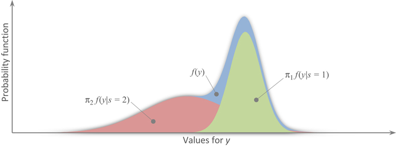
The chart is obtained from a simulated mixed Gaussian distribution with a probability π_1,2 equal to 0.5. The blue curve defines the RS distribution with 0.5 probability value for each regime. The red and green curves define the normalized distribution for the two regimes, turbulence (at left) and normal markets. (Matlab and Excel.)

$\{\begin{array}{c} P [s_{t} = 1] = \frac{1 - p_{22}}{2 - p_{11} - p_{22}} = π_{1} \\ P [s_{t} = 2] = \frac{1 - p_{11}}{2 - p_{11} - p_{22}} = π_{2} \end{array} where \sum_{j = 1}^{2} π_{j} = 1$ $\{\begin{array}{c} P [s_{t} = 1] = \frac{1 - p_{22}}{2 - p_{11} - p_{22}} = π_{1} \\ P [s_{t} = 2] = \frac{1 - p_{11}}{2 - p_{11} - p_{22}} = π_{2} \end{array} where \sum_{j = 1}^{2} π_{j} = 1$

(13.6)

$f (y_{t}) = π_{1} \frac{1}{\sqrt{2 π} σ_{1}} e^{(\frac{- {(y_{t} - μ_{1})}^{2}}{2 σ_{1}^{2}})} + π_{2} \frac{1}{\sqrt{2 π} σ_{2}} e^{(\frac{- {(y_{t} - μ_{2})}^{2}}{2 σ_{2}^{2}})}$ $f (y_{t}) = π_{1} \frac{1}{\sqrt{2 π} σ_{1}} e^{(\frac{- {(y_{t} - μ_{1})}^{2}}{2 σ_{1}^{2}})} + π_{2} \frac{1}{\sqrt{2 π} σ_{2}} e^{(\frac{- {(y_{t} - μ_{2})}^{2}}{2 σ_{2}^{2}})}$

(13.7)

In economics, Hamilton (1989) was the first to implement such a model in the attempt to study GDP. As Fig. 13.16 demonstrates, the RS model has the ability to capture the nonnormality of returns and therefore to better explain the Black Swan^f fat tail problem. High kurtosis is mostly present in long historical time series where the economy experiences a higher number of extreme returns. In other words, there is a higher probability of being under the tail (fat tails), and the standard deviation might not precisely capture the true risk involved. In fact, risk measures calculated on such assumptions can lead to erroneous interpretations.

3.6.3. Normality—Regime Switching Distribution

Earlier, we analyzed the concept of the normality of logarithmic returns. The results rejected the assumption of normally distributed returns due to high kurtosis and negative skewness. Nonnormality raises the pressure in gathering the correct conclusions about returns and risk, leading otherwise to erroneous and perhaps unsafe scenarios. To this extent, the RS model is tested to verify whether it effectively captures the peculiarities of returns.

The test results from the univariate regime switching model, as reported in Fig. 13.17, confirm the earlier results of nonnormality. In fact, the returns are better explained when the RS model is applied. The yellow line better traces the returns of each time series. Moreover, the percentage of data explained earlier each graph shows how the RS distribution percentage is closer to the one identified by real data. For example, in panel A, the normality probability distribution (ie, positive tails) explains 8.8%, whereas the threshold obtained from the observed data is only 5%. Hence, if we assume normality, the different likelihood of extreme returns can mislead the investor’s interpretation. On the other hand, considering the same 5% threshold value, the RS model explained 5.4%, describing a more accurate distribution. Analogous behavior occurs for the other time series.

Figure 13.17 Equity index—univariate RS probability distributions test.
The charts represent the distribution of the weekly returns of the equity under consideration. The histogram in blue represents the frequency distribution of the observed data. The red line instead identifies the normal distribution for the related variable. The yellow curve identifies the regime switching distribution with two states and transition probabilities defined by the univariate model. In the top of the graph, the confidence interval of the observed data at the top (in red) is compared with the one of the normal distribution in the middle (in black). In addition, the probability distribution values are given for the regime switching distribution (ie, in frontier markets, the observed values below −3.20% represent 5% of the overall data, whereas the normal distribution indicates 6.8% probability and the regime switching distribution 6.3%). (Matlab and Excel.)

3.6.4. Generalization—Multivariate Regime Switching

The univariate model is an effective method to define the peculiarities of stock returns. Nevertheless, in the case of portfolio construction, correlation among the assets needs to be identified. Due to the unconnected time-varying distribution of the returns, univariate models cannot fully integrate with each other. Multivariate regime switching models represent a possible solution to this problem.

$Y_{St} = μ_{St} + ɛ_{St}$ $Y_{St} = μ_{St} + ɛ_{St}$

(13.8)

$Y_{St} = (\begin{array}{c} y_{1, St} \\ ⋮ \\ y_{j, St} \end{array}) = (\begin{array}{c} μ_{1, St} \\ ⋮ \\ μ_{j, St} \end{array}) + (\begin{array}{c} ɛ_{St} \\ ⋮ \\ ɛ_{St} \end{array})$ $Y_{St} = (\begin{array}{c} y_{1, St} \\ ⋮ \\ y_{j, St} \end{array}) = (\begin{array}{c} μ_{1, St} \\ ⋮ \\ μ_{j, St} \end{array}) + (\begin{array}{c} ɛ_{St} \\ ⋮ \\ ɛ_{St} \end{array})$

(13.9)

$with t = 1, \dots, n and s_{t} = 1,2 and ɛ_{St} \sim NID (0, \sum_{st})$ $with t = 1, \dots, n and s_{t} = 1,2 and ɛ_{St} \sim NID (0, \sum_{st})$

$and, Σ_{s t} = (\begin{array}{c} σ_{1, 1, S t}^{2} & \dots & σ_{j, 1, S t}^{2} \\ ⋮ & ⋱ & ⋮ \\ σ_{1, j, S t}^{2} & \dots & σ_{j, j, S t}^{2} \end{array})$ $and, Σ_{s t} = (\begin{array}{c} σ_{1, 1, S t}^{2} & \dots & σ_{j, 1, S t}^{2} \\ ⋮ & ⋱ & ⋮ \\ σ_{1, j, S t}^{2} & \dots & σ_{j, j, S t}^{2} \end{array})$

(13.10)

The methodology and idea behind the model is the same as the one for the univariate system. The additional information, which makes this model more suitable, relies on the variance–covariance matrix calculation, identified by ∑_st (Eq. 13.9). Here, it is possible to calculate a common regime model by estimating, via maximum likelihood estimation, the mutual probabilities that best explain all the equities included in the regression.

It is assumed that the number of states does not change from the previous univariate model. Therefore, given s_t equal 1 and 2, the distribution of each variable maintains the same mixed distribution structure. Furthermore, the transition probability matrix governing the combination of the Gaussian distribution is the same across equities.

The multivariate estimation does not come without any cost. In fact, it is evident that in the attempt to create an overall two-period multivariate regime we have a partial loss of the distinctive characteristics of the equities.

3.6.5. Additional Evidence of Nonnormality

The results indicate that some information is lost in the attempt to standardize the regimes across the equities; however, as Fig. 13.18 illustrates, the differences between the univariate and multivariate unconditional probability distributions are minimal. For example, in frontier markets (panel A) the two curves almost perfectly overlay each other. As a result, both regime switching distributions outperform the simple Gaussian distribution. As a matter of fact, the percentages at the top of the graph highlight how the multivariate distribution has a higher power of fit when compared to the normalized distribution.

Figure 13.18 Multivariate RS probability distributions test.
The charts represent the distribution of the weekly returns of the equity under consideration. The histogram in blue represents the frequency distribution of the observed data. The red line instead identifies the normal distribution for the related variable. The yellow curve identifies the univariate regime switching distribution with two states and transition probabilities defined by the univariate model. The green curve identifies the multivariate regime switching distribution with two states and transition probabilities defined by the multivariate model. In the top of the graph, the confidence interval of the observed data at the top (in red) is compared with the one of the normal distribution in the middle (in black). In addition, the probability distribution values are given for the multivariate regime switching distribution (ie, in frontier markets, the observed values below −3.20% represent the 5% of the overall data, whereas the normal distribution indicates 6.8% probability and the multivariate regime switching distribution 4.9%). (Matlab and Excel.)

3.6.5.1. Correlation—Multivariate Regime Switching

The multivariate RS model incorporates the ability to capture the asymmetric correlation explained in the paper by Longin and Solnik (2001). In fact, Table 13.6 shows that the correlation in Regime 1 (ie, “bull markets”) is higher than the correlation discovered in Regime 2 (ie, “bear markets”). The results are in line with those uncovered by Ang and Bekaert (2002), who find that the RS model has the ability to partially identify the asymmetric correlation of returns.

Table 13.6

Multivariate Regime Switching Correlation

	Regime 1—bull markets
	MSCI Frontier Markets	MSCI Emerging Markets	MSCI United States	MSCI Europe
MSCI Frontier Markets	1.0000
MSCI Emerging Markets	−0.4784	1.0000
MSCI United States	−0.9170	0.6986	1.0000
MSCI Europe	−0.4910	0.8755	0.7935	1.0000

	Regime 2—bear markets
	MSCI Frontier Markets	MSCI Emerging Markets	MSCI United States	MSCI Europe
MSCI Frontier Markets	1.0000
MSCI Emerging Markets	−0.8074	1.0000
MSCI United States	−0.9799	0.7249	1.0000
MSCI Europe	−0.8731	0.8184	0.9078	1.0000

Source: Matlab calculations.

This table reports the correlation matrix calculated from the variance–covariance matrix obtained with the multivariate regime switching model. The range of colors highlights the degree of correlation between the time-series.

3.6.5.2. Number of Regimes

The number of regimes is particularly important since it defines the structure of the return distribution, which in turn sets the basis for the asset allocation optimization process. However, the choice is usually arbitrary and left to the author’s interpretation of the economic model.

In the literature there is evidence of different solutions, from the two-regime models of Schwert (1989) and Turner et al. (1989) to the three-regime models of Kim et al. (1998) and Rydén et al. (1998), and even up to the four-regime models implemented in the most recent paper of Guidolin and Timmermann (2005).

To interpret economically the number of regimes in the different models is quite straightforward. This particular study concentrates on the simplest case scenario in which the economy follows a two-regime model (“calm and turbulent” periods). This permits a more parsimonious structure, but, most of all, it permits one to easily associate the hidden Markov model results with the findings of Longin and Solnik (2001).

4. Frontier Markets—Univariate Regime Switching Application

In 1819 Jean Charles Léonard de Sismondi first introduced the idea of economic cycles, unknown before that period. From that date onward, the literature extended the notions regarding economic performances. In fact, economies constantly face periods of expansion and contraction. However, the size and entity of these cycles might be erratic and unpredictable. RS models attempt to capture and explain these patterns via a probabilistic method in an effort to construct a portfolio, which better captures volatility and fosters returns.

Fig. 13.19 denotes the particular structure of business cycles called “peaks and troughs.” The development of an economy is shaped by periods of expansion in which a peak is reached followed by a downturn where the bottom of the recession is touched. In univariate regime switching, markets can be characterized by several business cycles. In fact, the duration, magnitude, and period of occurrence diverge in each situation. Even if each country’s business cycle is defined by its own magnitude, certain markets tend to move together given their close relationship (eg, Europe and the United States).

Figure 13.19 Regime switching model fit—business cycle evidence.
The charts embody the regime model fitted for each single variable. The red line identifies the natural low return for the equity index, while the gray line represents the probability of switching between the regimes of turbulence and normality, 1 and 0 respectively. The gray areas instead are calculated by setting a 0.5 threshold for the probability calculated before, which more precisely embodies the turbulent periods. The blue line shows the pattern of prices; however, bear in mind that the shape is different among the time series and therefore is not comparable; it is instead included to see if regime switching matches the fluctuation in price.
News reported from the Financial Times:
Global financial markets suffered one of their most turbulent weeks of recent years. Emerging market equities endured their worst losing streak since the 1998 Russian debt crisis. The selling pressure hit its peak on Monday when trading was halted temporarily in India after Mumbai’s benchmark index crashed 10 per cent in a matter of hours.

(Matlab and Excel regression.)

For a portfolio manager, the business cycle greatly influences the behavior of the investment. In an international scenario, defensive countries that are less sensitive to global business cycles can prove beneficial for the investor’s portfolio by lowering the contagion risk. In fact, these offset countries will help to reduce the losses when the economy enters into a global recession. Figure 13.19, for example, shows that the European debt crisis in 2011 did not substantially affect frontier markets.

The mean and variance are particularly different in each state. Clearly, Regime 1 represents the “bull” state of the economy characterized by lower volatility and positive returns. In contrast, Regime 2 defines the “bear” state where market prices are more volatile and the average excess returns are negative in sign.

Emerging markets appear to be highly volatile, with a higher probability of extreme negative results. Conversely, frontier markets are described by a more stable scenario. In fact, Table 13.7 shows how emerging markets’ behavior is characterized by a greater variation of returns during downturns and a greater number of instances of regime switching if compared to other equity indexes. Regime probability is quite constant among financial series, with a 20.17% chance of being in “bear” markets and 79.64% of being in “bull” markets on average. The European index obtains a more generous result with a probability connected to “bear” markets of 15.16%. This suggests a more stable framework, but, in downturn economies, Europe seems to attain the worst performance, recording the lowest mean along with the highest volatility.

Table 13.7

Univariate Regime Switching Regressions

	MSCI Frontier Markets	MSCI Emerging Markets	MSCI United States	MSCI Europe
μ₁	0.23%	0.26%	0.32%	0.32%
μ₂	−0.16%	−0.79%	−0.52%	−1.50%
σ₁	1.42%	2.37%	1.76%	2.48%
σ₂	4.55%	6.83%	4.87%	7.24%
p₁₁ ^a	99.03%	98.22%	97.99%	98.81%
p₂₂ ^a	96.36%	92.69%	93.92%	93.57%
Regime 1 probability	78.93%	80.43%	75.14%	84.04%
Regime 2 probability	21.07%	19.57%	24.86%	15.16%
Regime 1 persistency^b	102.91 weeks	56.21 weeks	49.68 weeks	84.31 weeks
Regime 2 persistency^b	27.46 weeks	13.68 weeks	16.44 weeks	15.58 weeks

H₀: μ₁ = μ₂ ^c

0.0000

✓

Reject

null

0.0000

✓

Reject

null

0.0000

✓

Reject

null

0.0000

✓

Reject

null

H₀: σ₁ = σ₂ ^d

0.0000

✓

Reject

null

0.0000

✓

Reject

null

0.0000

✓

Reject

null

0.0000

✓

Reject

null

Source: Matlab and PcGive.

The table summarize the results for the weekly correlations among the MSCI equity indexes. The range of colors highlights the degree of correlation between the time-series.

$y_{t} = μ_{S t} + ɛ_{t}$ $y_{t} = μ_{S t} + ɛ_{t}$

where St is explained by an unobservable discrete Markov chain that assumes a two-states regime. The constant μ_St is IIN(0,1) among all assets. The results are obtained on a weekly basis from a 7-year period, 06/01/2007 to 05/30/2014 included.

^a The probabilities p₁₁ and p₂₂ represent the diagonal of the transition matrix. In particular, p₁₁ identifies the probability of being in Regime 1 at time t + 1 if at the current time we are in Regime 1. The same line of reasoning is employed for p₂₂.

^b The persistency indicates the average number of weeks each regime lasts.

^c The coefficient indicates the p-value for the relative null hypothesis tested against the alternative hypothesis, H₁: μ₁ ≠ μ₂, and ✓ indicates the rejection of the null hypothesis.

^d The portmanteau test is executed with 22 lags, which refers to the corrected version of the Box–Pierce test (1970), also called Q statistics. The test is designated as the goodness-of-fit test. The coefficient indicates the p-value of the test; above 0.05 we reject autocorrelation.

The persistency coefficient, measuring the average duration of each regime, supports the line of reasoning followed until now. In particular, emerging markets recorded average durations of 56.21 and 13.68 weeks for “bull” and “bear” markets, respectively. Conversely, for expansion periods the frontier markets average is twice as high, 102.91 weeks. Nevertheless, the average duration of turbulences is also higher, 27.46 weeks, suggesting longer-lasting downturn periods.

As a result, frontier markets highlight the attributes of a stable market that is mostly independent given its low correlation. Moreover, in downturn states of the economy, the markets embrace a good reaction with relatively low volatility and controlled means compared to other markets. Finally, the average periods outperform the MSCI United States Index, with longer averages for stability and shorter averages for instability.

4.1. The Importance of Asset Allocation

The importance of asset allocation is well known in portfolio management, in particular, with respect to security selection and timing. According to Barison et al. (1986), the asset allocation procedure accounts, on average, for 93.6% of the variation of returns over time, meaning that timing and security selection bear a 6.4% impact. Moreover, Blake et al. (1999) also discovered that variation in portfolios’ overall returns is highly explained by asset allocation; as much as 99.5% of variation is attributed to asset allocation in the UK market. Conversely, Kritzman and Page (2003) suggest that security selection leads portfolios to possible higher returns compared to the variation in asset allocation. However, the cost is that security selection might bear a higher risk, which might not comply with client objectives.

4.2. Generalization—Investor Optimization Problem

To solve the asset allocation problem in regime switching structures, we follow Guidolin and Timmermann (2005), utilizing a technique also implemented in Ang and Bekaert (2002). These papers explore the asset allocation optimization through maximizing the expected utility function within a multiperiod time horizon. Constant relative risk aversion (CRRA) utility function is implemented to calculate the appropriate weight of each MSCI equity index utilized in the portfolio.

Eq. 13.10 describes the investor utility preferences given the time horizon T. Thus, the numerator, W_{t + T}, defines the wealth invested at time t and held until time T. Furthermore, γ describes the investor risk aversion. As a result, if a simple buy-and-hold strategy is considered, the asset weights do not need to be rebalanced every period; therefore the system can be represented by Eqs. 13.11 and 13.12.

$u (W_{B}) = \frac{W_{t + T}^{1 - γ}}{1 - γ}$ $u (W_{B}) = \frac{W_{t + T}^{1 - γ}}{1 - γ}$

(13.11)

$W_{t + T} = (1 - {w^{'}}_{t} ι_{3}) \exp (T r_{f}) + {w^{'}}_{t} \exp \sum_{i}^{i = T} (r_{f} + r_{t + 1})$ $W_{t + T} = (1 - {w^{'}}_{t} ι_{3}) \exp (T r_{f}) + {w^{'}}_{t} \exp \sum_{i}^{i = T} (r_{f} + r_{t + 1})$

(13.12)

In the formulas, w_t identifies the weights for each stock involved, w_t = (w₁ … w_n)′; consequently, the coefficient

(1 - {w^{'}}_{t} t_{3})

$(1 - {w^{'}}_{t} t_{3})$

identifies the portion of the wealth allocated to the risk-free asset. Therefore, under the assumption of a buy-and-hold strategy, the investors’ optimization problem translates to:

$\max_{w_{t}} E [\frac{W_{t + T}^{1 - γ}}{1 - γ}]$ $\max_{w_{t}} E [\frac{W_{t + T}^{1 - γ}}{1 - γ}]$

(13.13)

To numerically solve the allocation problem, Guidolin and Timmermann (2005) implemented the Monte Carlo simulation methods for integral. Furthermore, they employed the Barberis (2000) approximation approach for integral in the expected utility function, which results in the maximization of the following problem:

$\max_{w_{t}} N^{- 1} \sum_{n = 1}^{N} \{\frac{{[(1 - ({w^{'}}_{t} ι_{3}) \exp (T r_{f})) + ({w^{'}}_{t} \exp (\sum_{T}^{i = 1} (r_{f, i} + r_{t + i, n})))]}^{1 - γ}}{1 - γ}\}$ $\max_{w_{t}} N^{- 1} \sum_{n = 1}^{N} \{\frac{{[(1 - ({w^{'}}_{t} ι_{3}) \exp (T r_{f})) + ({w^{'}}_{t} \exp (\sum_{T}^{i = 1} (r_{f, i} + r_{t + i, n})))]}^{1 - γ}}{1 - γ}\}$

(13.14)

This method permits us to embrace the predictability between the state economies. As a matter of fact, in Eq. 13.12 N represents the number of Monte Carlo simulations where for each simulation a particular investment time horizon T is set. The simulated N paths are drawn from a mixed distribution governed by the regime switching structure calculated throughout the models (Eqs. 13.8–13.10). In particular, the probability transition matrix previously discussed governs the likelihood of each regime occurring in the future time horizon t + 1. To increase the accuracy of the model, 30,000 Monte Carlo simulations are carried out, as recommended by Guidolin and Timmermann (2005).

4.3. Portfolio Framework

To study the exposure and determine whether the RSM can improve the overall investor position, three portfolios are constructed given the data set described earlier. In portfolio EF, the Markowitz methodology is applied to define the best stock combination given client-specific risk aversion γ equal 5. In this particular, the classical quadratic utility function is employed.

$% Optimal . Portfolio = \frac{Port . Mean - Risk . Free}{Investor . Risk . Adversion \times Port . Variance}$ $% Optimal . Portfolio = \frac{Port . Mean - Risk . Free}{Investor . Risk . Adversion \times Port . Variance}$

(13.15)

In portfolio RS, the multivariate regime switching along with the Guidolin and Timmermann (2007) asset allocation framework is implemented. The 30,000 possible paths generated with a Monte Carlo simulation are governed by the multivariate regime switching (Eqs. 13.8–13.10). Furthermore, a 104-week (2-year average) time horizon is assumed. Consequently, the utility maximization formula (Eq. 13.14) previously proposed is implemented on a simulated observation. In portfolio WA the simple weighted-average method is applied; this is also used as a benchmark for both the Markowitz process and the RSM.

In all portfolios, short selling is not allowed. The financial characteristics of this are not fully inherent with the objectives of this work. In fact, a full stand-alone study on short-selling forces in frontier markets is more suitable. Nonetheless, even without short selling, the Markowitz methodology presents some limitations in constructing the efficient frontier. In fact, in the attempt to obtain the lowest variance we do not consider the MSCI Emerging Markets Index in the scope of the analysis. This leaves the portfolio exposed to a few stocks only, compromising interpretation of the models. The same behavior appears in portfolio RS. Therefore, in the attempt to create a realistic situation in which the investor fully diversifies unsystematic risk, a restriction of just 2.5% minimum is set. This allows the creation of a more realistic international investment scenario due to the involvement of all equity indexes and, at the same time, a minimal interference with the methodology applied. However, this still leaves a few stocks dominating the others. In fact, the MSCI United States and MSCI Frontier Markets indexes seem preferable to both MSCI Europe and MSCI Emerging Markets indexes. This is understandable since the portfolio forces try to diversify the risk through the low correlation of frontier markets while optimizing to increase the return by investing in the incredibly outstanding performance of the United States over the past few years, reflected by the strong historical returns.

Furthermore, a common behavior across the model is that it shows a high exposure to the risk-free rate given the substantial fixed rate. In addition, the low risk, assumed to be zero for the purpose of the risk-free assumption, leaves this asset desirable if compared to some of the MSCI equity indexes. Hence, a static constraint of 15% (ie, Fig. 13.20) is set to allow the study to concentrate on how the models redistribute the weights among international assets and if the redistribution adds substantial value to the portfolio.

Figure 13.20 Portfolio distribution.
The graph represents the portfolio distribution for the three-asset case, and the constraint of 15% on the risk-free assets. It is evident how portfolios EF and RS lack redistribution among assets. In fact, one asset, the emerging markets, prevails over the others. In portfolio A there is no inclusion of frontier markets, but they are included in portfolio B. EF stands for efficient frontier methodology; RS stands for regime switching methodology; WA stands for weighted average methodology. (Bloomberg, Matlab, and Excel regression.)

Portfolio analysis can thus be a useful approach to underline the particular exposure to frontier markets. A portfolio’s performance will also allow the investor to comprehend how the investment behaves in an international framework and how it performs in relation to comparable benchmarks. The benchmarks have an important role within the evaluation since they establish boundaries that determine the reliance of the constructed portfolio. Consequently, this rests with the Standard & Poor’s (S&P) 500, a strongly influential international stock exchange. In addition, it is most suitable for the diversification of the position of a US citizen looking for international portfolio exposure. Alongside, the MSCI World Index is employed to see the exposure of the portfolio to the overall world, the most internationalized asset. The results underline how the US market and the MSCI World Index are strongly connected, with almost identical performance. This provides additional light on the strong influence of US markets on international portfolio exposure.

4.4. Results

Do frontier markets improve returns or lower variance? Are “frontier markets” desirable assets to invest in? The portfolio framework described is designed and tested on different time intervals to expand the notions related to “frontier markets exposure.”

In fact, the two time periods, historical (7 years) and actual (1 year), will help to recognize the effects of the evolution accomplished by frontier markets. Moreover, the relationship between portfolios A and B will reveal if significant value can be added in the portfolio structure by capturing additional information via the RS model. The first step consists of calculating the asset allocation given the specific models previously discussed.

The characteristics of frontier markets become clearer as the MSCI Frontier Markets Index is added to the portfolio, especially in the regime switching asset allocation method. This can be explained in the strong positive evidence related to these markets. In fact, even if overshadowed by the bullish US economy, frontier markets still find a space in the regime switching portfolio. Higher levels of diversification are in fact a desirable input for both the Markowitz methodology and the RS utility maximization process. Encouraging evidence is also found in the univariate RS model, where the estimates suggest low correlation to international distress and good transition probabilities.

Therefore the portfolio asset allocation suggests that both processes (Markowitz and regime switching) are expected to drive investments away from the MSCI United States Index and reallocate them into frontier markets. Nevertheless, in portfolio B, the Markowitz optimization process behaves differently from the RS model by redistributing everything to the MSCI United States Index. This can be explained by misunderstanding future possible outcomes as driven only by historical past returns and variances. In fact, the more flexible RS model rebalances the portfolio, capturing current frontier market positive returns and encouraging future potential returns. In fact, the simulation driven for 104 observations (2 years) throughout the 30,000 Monte Carlo simulations reported that frontier markets are less risky on average. On the other hand, Markowitz historical expected values preclude a greater investment to frontier markets, concentrating the investments unrealistically into a single best-performing stock.

By utilizing 7 years of historical results in portfolio A (Table 13.8), on one hand, Markowitz and RS models highlight insignificant differences in performance due to identical exposure to the US market. On the other hand, in portfolio B the RS model’s slightly higher exposure to frontier markets helps to reduce the volatility. Nevertheless, the portfolio underlines a lower performance in terms of returns per unit of risk due to the stable but constant growth when compared with the more speculative and outstanding growth of the US market.

Table 13.8

Historical 7-Year Portfolios Performances Outlook—Monthly Data Jun. 2007 to Jun. 2014

	Portfolio A			Portfolio B			Benchmarks
	Efficient frontier	Regime switching	Weighted average	Efficient frontier	Regime switching	Weighted average	S&P 500	MSCI World

Return	0.10%	0.10%	0.07%	0.10%	0.09%	0.06%	0.07%	0.07%
Std. dev.	2.47%	2.47%	2.77%	2.42%	2.23%	2.36%	2.89%	2.97%
Alpha [t-stat]	0.0003 [5.0429]	0.0003 [5.0429]	0.0000 [0.0364]	0.0003 [3.6915]	0.0002 [0.8746]	−0.0002 [−0.3093]	—	0.0001 [0.1266]
Beta	0.8531	0.8531	0.8744	0.8365	0.7614	0.7269	1.0000	0.9822
Adj. beta	0.9021	0.9021	0.9163	0.8910	0.8409	0.8179	—	0.9881
Sharpe ratio	0.0025	0.0025	−0.0099	0.0014	−00041	−0.0177	—	—
M2^a	0.10%	0.10%	0.10%	0.10%	0.10%	0.10%	—	0.10%
T2^a,c	0.05%	0.05%	0.01%	0.05%	0.04%	0.00%	—	0.01%
Information ratio^a	0.0897	0.0897	0.0054	0.0746	0.0318	−0.0061	—	0.0021
Client utility	0.0010	0.0010	0.0007	0.0010	0.0009	0.0006	0.0006	0.0007

Source: Datastream and recalculations.

The table reports the indexes for the past performances of the complete portfolios, obtained via combination of the optimal portfolio and risk-free assets. The benchmarks are relative to the S&P 500 data and the MSCI World Index. The pie chart represents the distribution of each portfolio. Notice that the blue part representing the risk-free assets is assumed constant at 15%. The red circle in the benchmark section indicates a portfolio fully invested in the relative index.

^a The coefficient is tested upon the S&P 500 benchmark, with a weekly average of 0.07% and weekly standard deviation of 2.89%.

^b The utility function used in the calculation is: $Utility = E (r) - 0.005 \times γ \times σ^{2}$ $Utility = E (r) - 0.005 \times γ \times σ^{2}$ .

^c The T2 is calculated on the adjusted beta since it will be more reliable in the long run.

The performance risk–diversification measure, M2, suggests no specific pattern. Instead, T2, which measures the risk premium per unit of systematic risk, beta, denotes a slightly better performance of portfolio B-EF. However, portfolio B-RS obtained a lower beta (0.76) compared to Markowitz (0.84), suggesting a lower market risk. In this case, a larger share held by frontier markets drove the portfolio away from the market portfolio risk measure, the S&P 500. Thus, due to similar Sharpe ratios but lower betas, frontier markets are internationally preferable to other MSCI indexes. The similar performance of the S&P 500 and the MSCI World indexes enhances our conclusions regarding frontier markets as a source of diversification.

In both portfolios A and B, the weighted-average methodology outlined the worst performance. However, it is important to remember that the more uniform distribution among the equity indexes suggests a possible healthier redistribution. In fact, all equities bear the same portion of risk among the different equity indexes. This fact supports the implementation of an RSM, if compared to the Markowitz process, due to its ability to better allocate the portfolio’s weights while capturing possible future opportunities.

The overall results of Table 13.8 support the United States’ positive historical period due to the attention of several economic actions aimed at relaunching the markets after the initial slow recovery from the financial crisis of 2007–09. The Markowitz and RS models highlight the difficulties of the BRIC countries in fostering their economies, rendering a flat return record over the past 5 years. We expect that the increase in technological and infrastructural development by frontier markets in the upcoming period will carry a greater level of stability and therefore a larger volume of investment with a consequently higher return per unit of risk for these markets.

Table 13.9 reports the results for the period Jun. 2014 to Jun. 2015, allowing us to better to capture the route followed by frontier markets and consequently to have a better picture of the actual portfolio exposure and portfolio opportunities. The weights used in developing the portfolios are the same as in the previous table.

Table 13.9

Actual 1-Year Portfolio Performance—Weekly Data Jun. 2014 to Jun. 2015

	Portfolio A			Portfolio B			Benchmarks
	Efficient frontier	Regime switching	Weighted average	Efficient frontier	Regime switching	Weighted average	S&P 500	MSCI World

Return	0.19%	0.19%	0.05%	0.17%	0.12%	−0.02%	0.18%	0.12%
Std. dev.	1.38%	1.38%	1.42%	1.34%	1.22%	1.23%	1.63%	1.55%
Alpha [t-stat]	0.0002 [2.4134]	0.0002 [2.4134]	−0.0010 [−1.1057]	0.0004 [1.0504]	−0.0004 [−1.5254]	−0.0016 [−1.6443]	—	−0.0005 [−0.8488]
Beta	0.8411	0.8411	0.7662	0.8210	0.7307	0.6162	1.0000	0.9130
Adj. beta	0.8940	0.8940	0.8441	0.8807	0.8205	0.7442	—	0.9420
Sharpe ratio	0.0689	0.0689	−0.0271	0.0611	0.0204	−0.0896	—	0.0162
M2^a	0.10%	0.10%	0.09%	010%	0.10%	0. 09%	—	0.09%
T2^a,^c	0.03%	0.03%	−0.11%	0.02%	−0.03%	−0.20%	—	−0.05%
Information ratio^a	0.0411	0.0411	−0.1597	−0.0053	−0.1151	−0.2058	—	−0.0378
Client utility^b	0.0019	0.0019	0.0005	0.0017	0.0012	−0.0002	0.0017	0.0012

Source: Datastream and recalculations.

^a The coefficient is tested on the S&P 500 benchmark, with a weekly average of 0.18% and weekly standard deviation of 1.63%.

^b The utility function used in the calculation is: $Utility = E (r) - 0.005 \times γ \times σ^{2}$ $Utility = E (r) - 0.005 \times γ \times σ^{2}$ .

^c The T2 is calculated on the adjusted beta since it will be more reliable in the long run.

It is noteworthy how in portfolio A, independent of frontier markets, the United States reported higher return-volatility patterns compared to the historical scenario. As expected, the higher exposure of Markowitz and RS models has captured the past good performance, precluding the possibility of capturing profit opportunities from other equity indexes. In this sense, the weighted-average portfolio faces a more diverse and complete portfolio, including a greater number of indexes. However, the relatively poor performance of all markets in 2015 compared to the US markets did not help to surge investment profits. The inclusion of frontier markets within the narrow time period brings diversification by reducing the overall standard deviation of the portfolio from 1.34% of the efficient frontier (EF) portfolio to the 1.22% of the RS portfolio. As a result, the volatility of developed markets appears to be fairly high when compared to frontier markets.

Furthermore, portfolio B has an overall lower performance when compared to portfolio A due to the lower exposure to US markets. The improvement of frontier markets investment is among the ways for risk diversification obtaining better exposure to risk and market trends. In fact, as mentioned previously, the change of investment direction from developed markets to frontier markets seems to have already taken place. The data have underlined that investors feel more confident and opportunities are becoming more and more concrete.

Across the subportfolios of B, the RSM has a lower exposure to systematic risk with a beta of 0.73, enhancing the abnormal return per unit of market exposure, 0.10%. Thus, the portfolio exposure in frontier markets seems to hinder a consistent international diversification. Investors looking at international opportunities should reconsider their distribution by embracing frontier markets in their positions.

Fig. 13.21 extends the analysis by directly comparing the actual with the historical outcomes of the portfolios. The performances tend to be particularly different between the two time periods. This is partly due to the long time period of observations for past results, where periods of booms and crisis affected the outcome, and partly due to the bull period of the United States and consequently the S&P 500. In fact, the S&P 500’s higher market return during 2014 is due to continuous bullish expectations. This was the main reason for the low and in some portfolios even negative information ratio in the current year. However, the inclusion of frontier markets did not strongly disrupt the performance of the portfolio.

Figure 13.21 Portfolios performance—comparison of 2007–14 versus 2014–15 (weekly data).
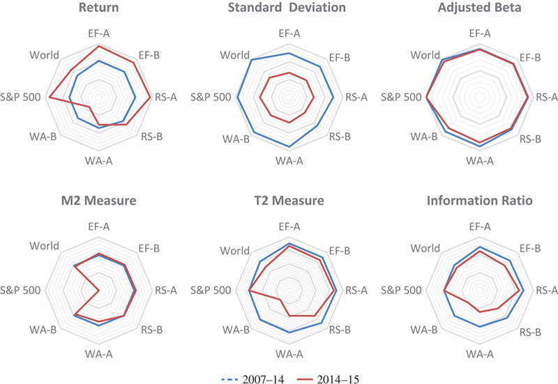
The graphs report the coefficients outlook for the two periods, 2007–14 in blue and 2014–15 in red. The T2 and information ratio are taken from the market benchmark, the S&P 500. In particular, adjusted beta is employed in the T2 measure. (Matlab, Datastream, and recalculations.)

In line with the results reported by Berger et al. (2013), frontier markets seem to have the ability to reduce the risk of an international portfolio in the mean-variance scenario. Their results suggest no lack of liquidity in trading volume. Therefore investors can easily access investment opportunities while remaining solvent in distress scenarios.

5. Conclusions

Frontier markets highlight interesting opportunities under different perspectives, from improvement of power supply and other technological development to advances toward a healthier society. Therefore positive investment prospects are present.

The BRIC countries have taught the new arrivals that careful decisions have to be made and that unconstrained development would lead to poor performance and eventually low investment income. For example, evidence of China’s lack of support for internal consumption partially led to its current growth slowdown. We argued that a country’s specific reaction to general policy enforcement is far from predictable, but investors’ ability to capture signals in the markets will determine part of the overall effect. Thus, careful and accurate decisions have to be accomplished by each country’s government.

Indicators of markets’ capitalization, corruption, and freedom suggest that frontier markets are growing by following the correct track. In fact, in most of the cases frontier markets have outperformed the BRIC countries. Moreover, the analytical study indicates interesting and desirable characteristics; in particular, frontier markets embrace low levels of volatility with fairly high returns. Clearly, in financial terms greater return is underlined by greater risk. In fact, frontier markets deal with a number of different types of risk which go beyond the concept of simple returns volatility. For instance, country risk, government instability, or regulatory risk can increase the pressure on single investments. Nevertheless, frontier markets are growing, and the data indicate that risk-adjusted returns are clearly on the bright side. Additionally, from a global investor point of view, the low correlation (0.38 on average) with other international countries represents a big advantage in a portfolio framework. We assume that the marginal relationship of the frontier stock markets can be the consequence of an early financial involvement which bound the country’s activities toward national consumption.

Longin and Solnik (2001) found that the correlation follows an asymmetric distribution in which international economic distresses intensify the relationships among financial markets. This result is extremely important for investors since diversification is most essential during downturn periods, and incorrect interpretations can lead to unexpected risky scenarios. Nonetheless, frontier markets still hold a good power of diversification even in turbulent time periods; conversely, emerging markets underline a strong relationship with both US and European markets, demonstrating a substantial international instability.

To further understand the true portfolio exposure of frontier markets, RS models are examined against Markowitz’s more static mean-variance portfolio optimization method. In fact, Startz and Nelson (1989) find time dependency in risk premiums, suggesting that future risk moves in a predictable fashion. Moreover, Schwert (1988) and Pagan and Schwert (1989) argue that the risk premium should allow a time-dependent variance with a predictable element.

Our RS model outcome is in line with Ang and Bekaert (2002a) finding where observed data obtained a better and more complete explanation and rejecting both the assumption of normality and standardized correlation. The power of RS to include the mixed Gaussian distribution for single time series allowed us to capture fatter tails and more extreme results along with the negative skewness of time series. Furthermore, the estimated values discovered by the multivariate regime switching allowed the Monte Carlo simulation to include the probabilities transition during the optimization process. This brought a change in the asset allocation process by better evaluating the future expectations of frontier markets. In fact, the historical link of the Markowitz optimization process precluded frontier markets opportunities by providing only a small portion of the investment to them. Indeed, the good historical performance of the US market (years of outstanding performance) bound the Markowitz methodology to allocate the biggest share of the investment to it.

The comparison between the 1-year actual and the 7-year historical performance shows how frontier markets still hold an increasing potential and a high power of market diversification. The negative characteristic is that both the RS model and the Markowitz process tend to expose the portfolio to particular assets, leaving a negligible investment in other assets, whereas the weighted-average method appears to allow a more rational distribution. This problem should not be underestimated from a client investment perspective.

To summarize, our findings indicate that frontier markets are evolving and are ready to accept investments. Opportunities are present, and diversification is achievable without major problems of liquidity pressure. Furthermore, in most of the results frontier markets appear to be preferable to well-known emerging markets. Markowitz portfolio optimization highlights the lack of capturing business cycles and possible future positive performance delineated by the probability estimates of the RS model. As a result, the RS model appears preferable to the Markowitz methodology. Additionally, the tests on correlation and normality embraced a higher power of fit under the RS model.

Finally, there are numerous applications around portfolio management and the RS model that can help to improve our results and enlarge the material on these early markets. In fact, a more advanced methodology which includes past information or time-varying probability can be used to discover additional information concerning frontier markets. Moreover, a focused study on the single MSCI Frontier Markets equity index can also be useful to understand, with more detail, which types of assets have the biggest impact on the returns, correlation, or currency risk. Thus, this chapter has attempted to set an analytical base for possible future studies which can further describe the particularities of frontier markets exposure (Fig. 13.22).

Appendix

A.1. Multivariate Regime Switching Model Fit

Figure 13.22 Multivariate regime switching model fit—business cycle evidence.
The graphs represent the regime model fitted for the two single variables. The red line identifies the natural log return for the equity index, while the gray line represents the probability of switching between the regimes of turbulence and normality, 1 and 0 respectively. The gray areas instead are calculated by setting a 0.5 threshold for the probability calculated before; this suggests the turbulence periods more precisely. The yellow area represents the regime switching for the multivariate regime switching method. As a matter of fact, the pattern is the same among all equities. The blue line shows the pattern of prices; however, bear in mind that the scale is different among the time series and therefore not comparable; it is instead included to see if regime switching matches the fluctuation in price. (Matlab and Excel regression.)

A.2. Reliability of Regime Switching Models

One of the peculiarities of RS models is the ability to capture turbulent periods of the economy. Perhaps, to not unconditionally accept this, a further test is implemented. In particular, Chow et al. (1999) identified a model to detect the turbulence in financial markets. Furthermore, the empirical results from Kritzman and Li (2010) advocate a good explanation when implemented on real data.

$d_{t} = (y_{t} - μ) \sum^{- 1} {(y_{t} - μ)}^{'}$ $d_{t} = (y_{t} - μ) \sum^{- 1} {(y_{t} - μ)}^{'}$

(A.1)

where d_t is the turbulence coefficient at a time t; y_t is the return of the time series at time t. This is a vector (1 × n) where in our case “n” is the number of industry sectors; μ is the simple average of historical return for each industry sector—thus a vector (1 × n); ∑⁻¹ is the variance–covariance matrix for the historical returns. This is represented by a matrix (n × n).

For more details regarding the calculation and the methodology applied, refer to Kritzman and Li (2010). In addition, look at the notes reported in Fig. 13.23.

Figure 13.23 Regime switching model—reliability test.
The graph represents the RS model fitted for the two single variables. The red line identifies the natural log return for the equity index. The gray areas are calculated by setting a 0.5 threshold for the smooth probability calculated by the RS model and represents the change in regime. The yellow areas identify the coefficient calculated with Eq. A.1.
Due to lack of data availability, the data set is not the same as the one described in Chapter 3. The same weekly frequency in utilized, but a narrower time period is involved (from Sep. 16, 2009, to Jul. 3, 2013). Furthermore, the turbulence coefficient is developed across the 10 industry sectors (energy, telecommunications, health, etc.). To fully explain the frontier markets, 30 companies were chosen from the MSCI Frontier Markets 100 Index in the same proportion to correctly match the behavior of the true index. Furthermore, these companies describe more than 66% of the returns; thus it was decided not to include more variables in the model. (Matlab and Excel regression.)

The idea is to overlap the turbulence coefficient, d_t, along with the regime switching outcome to see if the two results generate similar conclusions. It is clear that the period in which the coefficient demonstrates a higher result is captured by the RS model. The model captures some of the noise that the previous model did not capture. This is due to the different data set and the adoption of a smaller data set (fewer observed values). Therefore, the economy pushed the model to be more sensitive to smaller changes.

..................Content has been hidden....................

You can't read the all page of ebook, please click here login for view all page.

Table of Contents for Chapter 13: Frontier Market Investing: What’s the Value Add?

Create new playlist

Sign In

Sign Up

Abstract

Keywords

1. Introduction

2. Literature Review

2.1. International Markets

2.2. Frontier Markets

2.3. BRICs’ Lessons for Frontier Market Investing

2.4. Economic Evidence

2.5. Further Evidence

2.5.1. Technological Development

2.5.2. Energy Development

2.5.3. Health Development

3. Data and Methodology

3.1. Descriptive Statistics

3.2. Normality—Do Markets Behave “Normally”?

3.3. Correlation—Frontier Markets and Diversification

3.4. The Power of Diversification: Does Correlation Matter?

3.5. Correlation Extension—True Exposure

3.6. Frontier Markets and Regime Switching Model

3.6.1. Generalization—Univariate Regime Switching

3.6.2. Hidden Regime Switching—Markov Chain

3.6.3. Normality—Regime Switching Distribution

3.6.4. Generalization—Multivariate Regime Switching

3.6.5. Additional Evidence of Nonnormality

3.6.5.1. Correlation—Multivariate Regime Switching

3.6.5.2. Number of Regimes

4. Frontier Markets—Univariate Regime Switching Application

4.1. The Importance of Asset Allocation

4.2. Generalization—Investor Optimization Problem

4.3. Portfolio Framework

4.4. Results

5. Conclusions

Appendix

A.1. Multivariate Regime Switching Model Fit

A.2. Reliability of Regime Switching Models

Table of Contents for
Chapter 13: Frontier Market Investing: What’s the Value Add?

References

Ang A, Bekaert G. International asset allocation with regime shifts. Rev. Financ. Stud. 2002;15(4):11371187.
Ang A, Bekaert G. Regime switches in interest rates. J. Bus. Econ. Stat. 2002;20(2):163182.
Barberis NC. Investing for the long run when returns are predictable. J. Finance. 2000;55:255264.
Bekaert G, Urias MS. Diversification, integration and emerging market closed-end funds. J. Finance. 1996;51(3):835869.
Bender J. Portfolio of risk premia: a new approach to diversification. J. Portfolio Manage. 2010;36(2):1725.
Berger D, Pukthuanthong K, Yang J. Is the diversification benefit of frontier markets realizable by mean-variance? The evidence of investable funds. J. Portfolio Manage. 2013;39(4):3648.
Bodie Z, Kane A, Marcus AJ. Investments. ninth ed. New York: McGraw-Hill; 2009.
Chen, J.S., Ang, A., 2001. Asymmetric Correlations of Equity Portfolios. EFA Barcelona Meetings.
Chua DB, Kritzman M, Page S. The myth of diversification. J. Portfolio Manage. 2009;36(1):2635.
Covrig, V., Ng, L., Chan, K., 2004. What Determines the Domestic Bias and Foreign Bias Evidence from Equity Mutual Fund Allocations Worldwide. EFA 2004 Maastricht Meetings Paper No. 2527.
Dahlquist, M., Harvey, C.R., 2001. Global Tactical Asset Allocation. SSRN.
Das SR, Uppal R. Systemic risk and international portfolio choice. J. Finance. 2004;59(6):28092834.
Guidolin M, Timmermann AG. An econometric model of nonlinear dynamics in the joint distribution of stock and bond returns. J. Appl. Econom. 2005;21:122.
Guidolin, M., Timmermann, A.G., 2005b. “Strategic Asset Allocation and Consumption Decisions under Multivariate Regime Switching.” Working Paper 2005-2B, Federal Reserve of St. Louis.
Guidolin M, Timmermann AG. Asset allocation under multivariate regime switching. J. Econ. Dyn. Control. 2007;31(11):35033544.
Guidolin M, Timmermann AG. International asset allocation under regime switching, skew, and kurtosis preferences. Rev. Financ. Stud. 2008;21(2):889935.
Hamilton JD. A new approach to economic analysis of non-stationary time series and the business cycle. Econometrica. 1989;57(2):357384.
Hamilton JD. Analysis of time series subject to changes in regime. J. Econom. 1990.
Hamilton JD. Time Series Analysis. Princeton, NJ: Princeton University Press; 1994.
Hamilton, J.D., 2005. Regime-Switching Models.
Jayasuriya SA, Shambora W. Oops, we should have diversified! Appl. Financ. Econ. 2009;19(22):17791785.
Kim MJ, Nelson CR, Startz R. Testing for mean reversion in heteroskedastic data based on Gibbs-sampling-augmented randomization. J. Empir. Finance. 1998;5(2):131154.
Kritzman M, Li Y. Skulls, financial turbulence, and risk management. Financ. Anal. J. 2010;66(5).
Kritzman M, Page S, Turkington D. Regime shifts implications for dynamic strategies. Financ. Anal. J. 2012;68(3).
Longin F, Solnik B. Is the correlation in international equity returns constant: 1960–1990? J. Int. Money Finance. 1995.
Longin F, Solnik B. Extreme correlation of international equity markets. J. Finance. 2001;56(2):649676.
Maginn JL, Tuttle DL, Pinto JE, McLeavey DW. Managing Investment Portfolios: A Dynamic Process. third ed. Hoboken, NJ: John Wiley & Sons; 2007.
Schaller H, Van Norden S. Regime switching in stock market returns. Appl. Financ. Econ. 2010.
Speidell L, Krohne A. The case for frontier equity markets. J. Invest. 2007;16(3):1222.
Turner, C.M., Startz, R., Nelson, C.R., 1989. A Markov model of heteroskedasticity, risk and learning in the stock market. NBER Working Paper No. 2818. J. Financ. Econ. 25, 3–22.
Welch LR. Hidden Markov models and the Baum–Welch algorithm. IEEE Inf. Theor. Soc. Newslett. 2003;53(4).