Chapter 7

Measuring Market Risk in the Light of Basel III: New Evidence From Frontier Markets

A. Burchi
D. Martelli    Department of Economics, University of Perugia, Perugia, Italy

Abstract

The recent 2008–09 financial crisis has led international financial authorities to review the existing regulations in order to strengthen the risk coverage of the capital framework. These reforms will help to raise capital requirements for the trading book, which represents a major source of losses for international financial institutions, especially during crisis periods. In particular, the Basel Committee on Banking Supervision has introduced a stressed value at risk (SVaR) capital requirement as a new methodology to evaluate market risk. This chapter focuses on frontier markets and aims to compare five different models evaluating market risk, highighting potential issues that banks have to face while calculating the amount of SVaR for their investments. It emerges that frontier markets, showing an interesting risk–return profile and presenting a low correlation level with the European and the US markets, allow international investors to improve their asset allocation while simultaneously containing the cost of capital requirements.

Keywords

stressed value at risk
market risk
frontier markets
capital requirements
Basel Committee on Banking Supervision

1. Introduction

The recent 2008–09 financial crisis has led international financial authorities to rethink the current regulations, since banks were unable to meet market losses, as the capital was not sufficient to cover unexpected losses in extreme adverse events. In certain situations, the shortage was so extensive that goverments had to bail out many financial institutions. The current framework, establishing the value at risk as the official measure of market risk, has shown its limits, especially in the presence of extreme negative market conditions. The Basel Committee on Banking Supervision (BCBS) has thus started to review the pillars of the Basel Accord, focusing on strenghtening the capital requirements for the trading book, which represented a major source of losses during the crisis. In particular, the BCBS has introduced a stressed value at risk (SVaR) capital requirement, which consists in the implementation of several VaR parametric models in order to take into account multiple sources of risk.
While the number of studies analyzing this approach in developed countries has grown quite rapidly, the field of research focusing on frontier markets is still limited. The chapter aims to bridge this gap by comparing five different models and highighting potential issues that banks have to face while calculating the amount of SVaR for investments in frontier markets. It emerges that frontier markets show an interesting risk–return profile and present a low correlation level with the European and the US markets. Both factors allow international investors to improve their asset allocation while simultaneously containing the cost of capital requirements.
The chapter is structured as follows: Section 2 summarizes the literature discussing the advantages and limits of the use of VaR methodologies as methods to estimate market risk. Section 3 presents five estimation models related to VaR methodologies and discuss the opportunity cost of regulation for financial institutions. Section 4 analyzes the empirical results of the effects of the new capital requirements for market risk in the investment decision making of banks in frontier markets. Section 5 presents some concluding remarks and considers future developments.

2. Literature Review

The BCBS has proposed different measures of market risk, despite its preferred tool for assessing the exposure of financial institutions to market risk is the value at risk (VaR). VaR is a measure of the potential maximum loss in the value of a portfolio. In particular, 99% VaR is the loss, which is likely to be exceeded only 1% of the time.
However, in response to the 2008–09 financial crisis, the BCBS has started a comprehrensive set of reforms, aiming to strengthen the capital requirements of financial institutions previously stated in the so-called Basel II Accord. Quantitative revisions of such accords (better known as Basel 2.5 and Basel III) (Basel Committee on Banking Supervision, 2011a,b) are focused on creating a greater resilience in individual banks and financial institutions, so as to reduce systemic crises. In particular, a source of risk that has been put under investigation is the trading book, since the model used did not correctly take into account the possibility of a systemic crisis. That is why, among the quantitative standards, the revised ones mainly concern the minimum historical period for the VaR calculation and the minimum frequency of data set updating.
Unfortunately, traditional VaR analysis shows several limits. Three issues in particular are crucial (see Rockafellar and Uryasev (2002) and Nielsson (2009) for a comprehensive review of VaR’s weaknesses). First, VaR assumes that market returns are normally distributed, whereas the empirical evidence suggests that returns follow a leptokurtic distribution; in other words, the tails of the market distribution are fatter compared to those in the normal distribution (among others, Pafka and Kondor, 2001). Second, VaR analysis does not provide any information regarding the shape of the extreme left tail of the distribution after that specific value of loss, although this information would be very helpful, especially in the case where market returns are not normally distributed, like they actually are. Third, traditional VaR analysis does not always fully take into account the benefits of portfolio diversification. Although the first issue can be solved by recalibrating the parameters according to a more leptokurtic distribution, such as a logistic distribution (Chen, 2012), the other two issues remain open.
Unfortunately, also comparing different methodologies (traditional VaR, stressed VaR, and expected shortfall), it seems that it is not possible to identify any alternative, which is limit-free (Chen, 2014). For example, while the expected shortfall, determined by the average of all losses exceeding the VaR level, has the property of subadditivity (but VaR does not), expected shortfall cannot be backtested, whereas VaR allows forecasts to be easily compared with historical observations (Hull, 2012). Thus, despite its limitations, the possibility to run backtests makes VaR the preferred alternative for measuring market risk, both for financial authorities and for institutions (Macchiarola, 2009).
Unfortunately, Nocera (2009) states that summarizing the whole statistical distribution with just one number can be problematic and lead to possible misunderstandings. Behavioral factors, in particular the anchoring effect, can also play an important role if VaR is perceived by traders or executives as a point of reference, such as the specific amount of risk that a bank is willing to bear over a certain time horizon (Taleb, 2009). In order to maximize the overall return, traders can in fact align the risk of their portfolios to the same level of VaR set at the company level, while executives can have a false sense of security since they are not interested in considering what could happen in the extreme left part of the tail (Einhorn, 2008). These behavioral issues affecting both traders and corporate executives could (at least partially) explain why financial institutions tend to generally disclose two levels of VaR: stating a higher forecast of risk than what is actually observed for external (ie, regulatory) use, while adopting a lower level for internal use. This behavior can also be justified by the desire to avoid inspections or worse sanctions by financial regulators (Pérignon et al., 2008). Another possible explanation why it is prudential to adopt a conservative level for internal use is that VaR analysis is likely to fail during periods of market stress. For this reason, financial regulators have proposed in a recent revision of the Basel Accord a stressed version of VaR analysis (Basel Committee on Banking Supervision, 2011b). The revised VaR methodology subjects the traditional model to a continuous 12-month period of significant financial stress, in order to obtain a more significant threshold, especially during periods of market stress.
Thus, the stressed VaR seems nowadays to be one of the best possible compromises between analytical rigor in thinking and its practical implementation and easy interpretation. As far as peer practices regarding the models used, the majority of banks utilize historical simulations and apply both the absolute and the relative measures of volatility for different risk factors. Despite this is the easiest way to implement a stressed VaR, using historical data cannot ensure superior results, since past performance is not a guarantee of future returns, of course.
Our study involves advanced methodologies that are able to detect with greater care the dynamics of risk, limiting the computational complexity. Parametric models are also consistent from an operational perspective, despite financial institutions continuing to adopt in practice models which are too simple to take into adequate account all risk factors.
Our chapter differs from other studies in literature for two main reasons. First, differently from previous work focusing on a very limited number of frontier economies, our research analyzes all 25 frontier markets, according to the classification proposed by the FTSE (2014). Second, the use of an opportunity cost function allows the analyst to determine the reduction in profits resulting from the rules of prudential supervision. Financial institutions should thus be able to better capture potential benefits from investing in these countries.

3. Value at Risk and the Capital Requirement for Market Risks

3.1. Defining Value at Risk

Value at risk (VaR) is a measure that quantifies the level of risk associated with an investment. VaR is applicable to all types of assets: stocks, bonds, derivatives, currencies, and more. Specifically, the VaR estimates the maximum potential loss that a position could suffer on a specific holding period h and given a certain level of confidence α, typically 99 or 95%.
Hence, to estimate the VaR at time t we need to find the α quantile of the discounted h-day profit and loss (P&L) distribution. Given a sequence of prices of a financial asset (S0, S1, …, Sn), the returns during the period t will be:

Rt=lnStSt1

image(7.1)
where Rt is the return between the period t − 1 and t. It is possible to decompose the time series of log return every time t in a component part of a predictable C1(t) and unpredictable (random) C2(t). Then:

Rt=C1(t)+C2(t)=E(Rt|It1)+εt

image(7.2)
The random variable has a component given by the conditional mean E(Yt|Ft1)image, where Ft−1 is the set of information available at the time t − 1, and a random component ɛt. Therefore, the distribution of Rt depends on the random variable ɛt. We can assume that it follows a distribution so described:

ɛt=D(μt,σt2)

image(7.3)
where μt and σt2image are the conditional mean and the variance of ɛt and may be estimated through a variety of parametric models, semiparametric and nonparametric. It follows that the VaR for the variable can be calculated as follows:

VaRt=E(Rt|Ft1)ασt

image(7.4)
where α represents the critical value of the distribution ɛt to achieve the desired confidence level. It is possible to replace σt with alternative measures of conditional variance (Degiannakis et al., 2012).

3.2. VaR Estimation in the Banking Regulation

According to the Basel Committee, the daily capital requirement should be determined based on the higher level of either the previous day’s VaR or the average VaR of the prior 60 days multiplied by a correction factor with a 10-day holding period and a 99% confidence interval. Formally, the capital requirement can be written as follows:

CRt=maxVaRt1,(3+kt)160i=160VaRti

image(7.5)
where CR is the capital requirement, VaRt−1 is the daily VaR estimated decadal based on the previous day, (3 + kt) is the multiplication factor, and 160i=160VaRtiimage is the average VaR of the past 60 trading days.
The multiplication factor k depends on the result of a procedure for backtesting focusing on the number of violations, the cases in which the loss exceeds the VaR during a period of a year (verified at least quarterly). As shown in Fig. 7.1, the minimum multiplication factor is equal to 3, which compensates for any errors that may be related to the difficulty of implementing the estimation model, such as oversimplifications, rounding, distortions, and errors due to sample aggregation processes of different positions (Jiménez-Martín et al., 2009).
image
Figure 7.1 Multiplication factor based on violations. (Source: Basel, 2009.)
The revisions to the market risk framework (Basel 2.5) introduce the stressed VaR (SVaR), a measure of market risk tailored to stressed market conditions. Banks must compute the SVaR value that would replicate the standard VaR over a period when the relevant market factors are in distress, not shorter than 1 year. Analytically, the minimum capital requirement is:

CRt=maxVaRt1,(3+kt)160i=160VaRti+maxsVaRt1,(3+kt)160i=160sVaRti

image(7.6)
As in the previous version, the correction factor depends on the result of the backtest. The SVaR is an additional capital requirement to the one currently in force and not a substitute for it. This leads to a considerable increase in the capital requirement.
Regarding the estimation method for the VaR estimate, the Basel Committee does not put constraints. However, the Committee emphasizes that the choice should fall on a model able to capture all market risks that the bank faces (Basel Committee on Banking Supervision, 2004).
The Committee defines only guidelines and criteria for the assessment and dissemination of VaR. The legislation imposes the holding period (10 days); the length of the historical time series of observations, which must not be shorter than 1 year (252 trading days); and the confidence level (99%). With regard to the depth and refresh rate of the time series used for estimation, the Basel Committee expects that the first is at least 1 year, and states that the refresh rate is at least 3 months (European Banking Authority, 2012).

3.3. The Estimation Models

In the analysis, we adopt five different models to estimate:
1. The historical simulation models (HS)
2. The parametric models (PM)
3. The GARCH(1,1) models (GM)
4. The EWMA models (EM)
5. The TGARCH(1,1) models (TGM)
The Basel Committee explicitly stated the first two methods. The types 3, 4, and 5 are more complex to use, but they allow estimates of higher precision to be obtained.

3.3.1. Historical Simulation Models

The HS model assumes that the distribution of future returns is constant over time and corresponds to the observed distribution. Given a certain distribution in the previous n observations, it is easy to extract the desired percentile (eg, in a vector of 250 observations, the 99th percentile corresponds to the third worst result).

3.3.2. Parametric Models

The PM approach is well known for its ease of calculation and understanding. The model assumes a normal distribution of returns Rt. The VaR observed in the period t is thus:

VaR=μZ(α)σ

image(7.7)
The VaR is calculated considering estimates of mean and standard deviation of the normal distribution as well as associated values Z(α).

3.3.3. GARCH Models

We can consider the conditional mean of the returns an autoregressive process of order k, AR(k):

E(Rt|It1)=v0+i=1kviYt1

image(7.8)
The component ɛt is not predictable, and it can be expressed as an ARCH process:

ɛt=ztσt

image(7.9)
where zt is the set of independent and identically distributed random variables (0,1), while σt the standard deviation of conditioning ɛt. Engle (1982) introduced the ARCH (q) and expresses the conditional variance as a linear combination:

σt2=α0+α1ɛt12++αqɛtq2=α0+i=1qαiɛti2

image(7.10)
with α0 > 0 and αi ≥ 0 for i = 1, …, q.
The GARCH model results in a generalization of the ARCH model proposed by Bollerslev (1986). Assuming that the conditional variance depends on the number of squares of the errors ɛt2image, and from the series of the variances σt12,σt22,...,σtp2image. The series σt2image according to the GARCH (p,q) equates:

σt2=α0+α1εt12++αqεtq2+β1σt12++βpσtp2=α0+i=1q αiεti2+i=1p βiσti2

image(7.11)
with α0 > 0, αi ≥ 0 for i = 1, …, q β0 > 0, βj ≥ 0 for j = 1, …, p.
The GARCH model effectively captures some aspects of financial time series, such as the phenomena of volatility clustering and fat-tailed distribution (He and Terasvirta, 1999).

3.3.4. EWMA Models

A special case of the GARCH family model is the exponentially weighted moving average (EWMA). The volatility of the time t is a weighted average of the estimated volatility and the square of the previous error parameter. The variance of returns is a process with exponential decay:

σt2=λσt12+1tɛt12

image(7.12)
The EWMA model is a particular case of GARCH(1,1) with intercepts equal to 0, and the sum of the two remaining variables equal to 1. We use a λ equal to 0.94.

3.3.5. TGARCH Models

Brooks and Persan (2003) show that VaR models, taking into account the asymmetry of the distributions, tend generally to produce more accurate estimates. TGM gives different weights to the positive observations than to the negative ones. Analytically:

σt2=α0+i=1qαiɛti2+γɛt12dt1+j=1pβjσtj2

image(7.13)
where dt is a dummy variable that takes value 1 if ɛt < 0, and 0 elsewhere.
The coefficient γ measures the differential impact on the conditional variance to negative events. The expected sign of γ is positive; then the volatility is higher in correspondence to negative detections and increases as the dispersion of standard deviation.

3.4. The Opportunity Cost of Regulation

From a managerial viewpoint, the estimate of the expected loss should allow the bank to allocate enough capital to be protected from the risk, trying, at the same time, to avoid excess distraction of capital from profitable activities.
We do not intend to propose an evaluation of estimation models. We want to investigate the effect of different models in the application of regulatory capital in the context of frontier markets. In order to do that, we introduce a cost function that focuses on the performance not achieved, due to the capital subtracted to the trading activity. We define the reserve in excess (ERt) in time t as the capital unnecessarily subtracted from the activity. Thus, we set the opportunity cost OCt equal to:

OCt=ERt×rptf

image(7.14)
with rrf equal to the return of the investment portfolio during the period t.
Concerning the quantification of excess reserves, after we estimate the capital that banks must allocate, we can calculate the excess reserves. In the case of negative returns, the excess reserve ER is the distance between the return (negative) and the levels of capital set aside. The larger the difference, the greater the portion of the capital subtracted “needlessly” to investment. In the case of VaR violation we do not have an excess, but a lack of reserves that does not generate an opportunity cost. In the case of positive returns, the opportunity cost is due to the entire reserve. Fig. 7.2 shows the difference between the two cases. Analytically:

ERt=DPtmin0;rt0ifDPt<rtifDPtrt

image(7.15)
image
Figure 7.2 Excess reserves.

4. The Results of the Empirical Analysis

4.1. Investment Opportunity in Frontier Markets

Our data consist of the returns of the stock market index of the frontier market countries according to the classification proposed by FTSE (2014). The data cover an observation period of 20 years, from Sep. 1, 1995, to Aug. 30, 2015, for a total of 5217 trading days. We downloaded from Datastream all time series used in the study (data type PI). Unfortunately, historical time series are not available for all the countries under investigation from the same starting date. Table 7.1 shows the index selected and the beginning of the observations. To allow a proper comparison of the results, we also use index data representing the US market and the European market.

Table 7.1

Emerging Countries Considered in the Analysis Sample, Benchmark Index of the Stock Markets and Starting Date of the Observations

Country Index Start date
Argentina Argentina Merval 09/07/1995
Bahrain Bahrain All Share 01/02/2003
Bangladesh Bangladesh DSE 30 01/28/2013
Botswana Botswana SE DMS Cos. Idx. 05/01/2001
Bulgaria Bulgaria SE SOFIX 10/20/2000
Côte d’Ivoire S&P Côte d’Ivoire BMI 07/30/2008
Croatia Croatia CROBEX 01/02/1997
Cyprus Cyprus General 09/03/2004
Estonia OMX Tallinn (OMXT) 06/03/1996
Jordan Amman SE Financial Market 09/07/1995
Kenya Kenya Nairobi SE (NSE20) 09/07/1995
Lithuania OMX Vilnius (OMXV) 01/03/2000
Macedonia Macedonian SE MBI 10 01/03/2005
Malta Malta SE MSE 05/14/1998
Mauritius Mauritius SE SEMDEX 09/07/1995
Nigeria Nigeria All Share 01/14/2000
Oman Oman Muscat Securities Mkt. 10/22/1996
Qatar Qatar-DS 01/01/2004
Romania Romania BET 09/19/1997
Serbia Belgrade BELEX Line 12/25/2006
Slovakia Slovakia SAX 16 09/07/1995
Slovenia Slovenian Blue Chip (SBI Top) 03/31/2006
Sri Lanka Colombo SE All Share 09/07/1995
Tunisia Tunisia TUNINDEX 01/01/1998
Vietnam Ho Chi Minh SE Vietnam Index 0728//2000
EU Euro Stoxx 50 09/07/1995
USA S&P 500 09/07/1995
Before analyzing the quantification of capital requirements resulting from different evaluation models, it is appropriate to verify the investment potential of frontier markets.
Fig. 7.3 shows a graphical representation of the risk–return profile of a sample of the countries under investigation.a The space mean variance is useful for our purpose. We divide our analysis into three periods: the whole observation period, the crisis period (from Jan. 2008 to Dec. 2012), and the era since the global financial crisis (from Jan. 2013 onward).
image
Figure 7.3 Graphic representation, in mean-variance space, of market indices.
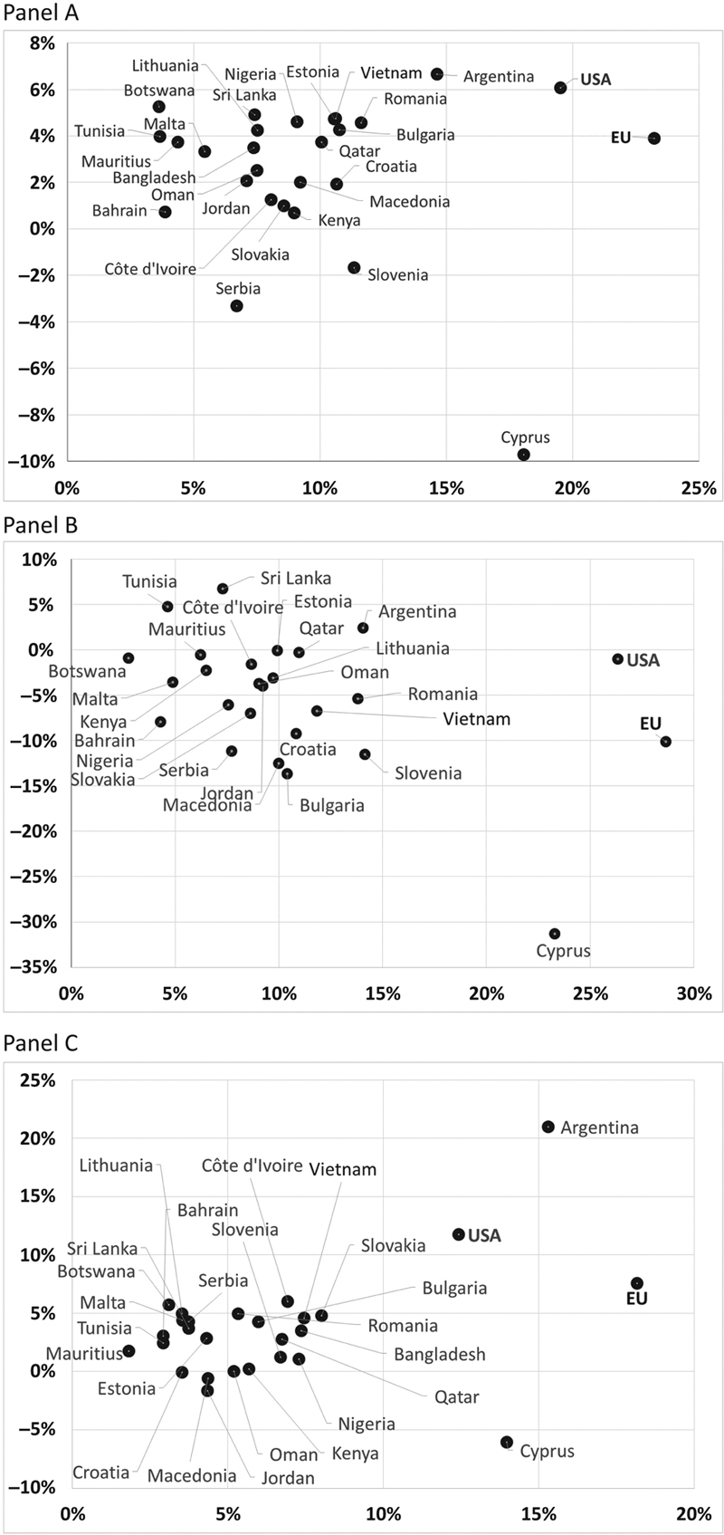
Panel A, complete sample; panel B, crisis period 2008–12; panel C, Post-Crisis Era.
In the definition of frontier markets are included countries whose characteristics are sometimes unique; data reflect this diversity. In Panel A, we observe some interesting empirical evidence. The risk–return profile of Cyprus is the worst and will not change in the other horizons of analysis. The frontier markets have different levels of performance, but surprisingly they all show a risk level significantly lower than that of developed markets.
Even more interesting are the data of the crisis period (2008–12) shown in Fig. 7.3 Panel B. The financial market crisis involves levels of return becoming negative, or close to zero, for all markets with the exception of Tunisia, Sri Lanka, and Argentina. Cyprus has been confirmed as the worst-performing country. Even in this period the frontier markets show a risk level considerably lower than the markets of Europe and the United States.
Fig. 7.3 Panel C shows the postcrisis period to the present day, about 3 years. The focus allows us to evaluate the ability to recover from the period of bear markets. The frontier countries offer unexpected empirical evidence, even when looking at the latest data. The European and the US markets again show much higher risk levels compared to the frontier markets. However, the latter have greater difficulty in recovering the precrisis levels with an average annual performance less than 7%. The United States and Europe show higher returns but at the cost of increased volatility, and the data also shows the difficulty of recovery for the economies of the old continent. In the postcrisis period, frontier markets seem to represent a very attractive risk–return alternative asset class, leading us to affirm the possibility of exploiting this opportunity in a perspective of portfolio diversification.
Finally, Table 7.2 shows the correlation matrix between the indexes analyzed. For reasons of space, we only report the data for the whole period. Even though we are far from the results of an optimization model, the table proves the concrete potentiality to benefit from the frontier markets in a perspective of risk diversification.

Table 7.2

Correlation Matrix of the Returns of Emerging Markets Analyzed

image

In dark gray high correlation, in white low or negative correlation.

4.2. The Capital Requirement and VaR Models within the Context of Frontier Markets

This section presents the results of our risk assessment. In order to estimate the stressed VaR, we need to identify a period of stress in financial markets. Our observation period is particularly extended, and thus we can identify several moments of bear markets. More precisely, we selected three stock market crashes: the 1997 Asian financial crisis (Jul. 2, 1997), the 2002 stock market downturn (Oct. 9, 2002), and the recent financial crisis of 2007–08 (Sep. 16, 2008).
Fig 7.4 show the graphic representation of the estimates of VaR and capital requirements in Nigeria, Argentina, Qatar, and Romania, the countries of the sample with the largest gross domestic products (GDPs).
imageimageimageimage
Figure 7.4 Graphs of the daily VaR and capital requirement estimated with different models.
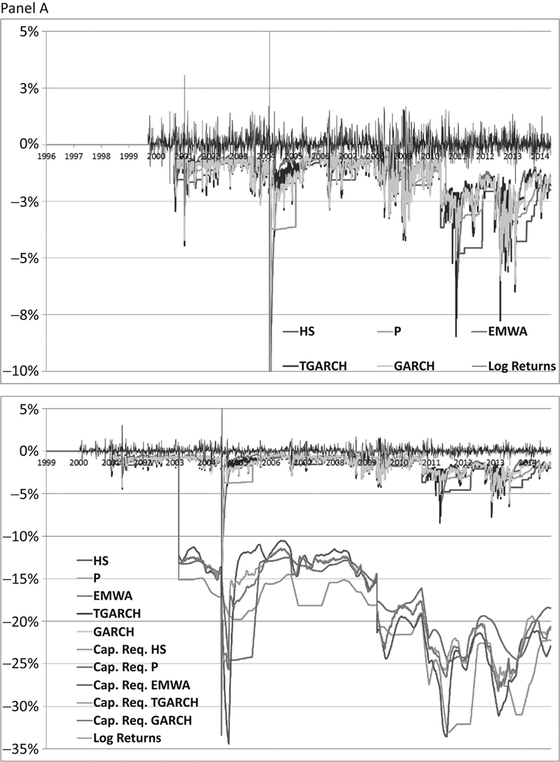
Panel A, Nigeria; panel B, Argentina; panel C, Qatar; panel D, Romania.
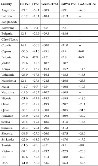
The charts show the difference between VaR and the requirement for prudential regulation. Apparently, the legislator was motivated to ensure a high capitalization of financial intermediaries while ignoring the good estimate of potential losses. Regarding the various procedures for estimating VaR, the models EM, GM, and TM show more approximation ability at the cost of greater complexity of implementation.
The charts indicate the noteworthy increase in volatility during the period of market stress, the simultaneous worsening of the VaR estimates and associated capital requirements. At the occurrence of a crisis, in line with the regulation, we updated the crisis period in SVaR estimation. The graphs can detect such changes.
The slight distance between the lines of the capital requirement indicate a sort of flattening of differences between the models. This increases the importance of the choice of the reference period instead of the model. In this sense, the stressed VaR risk, in its implementation, is an instrument formally rigorous but with a “difficult rationale.”
Table 7.3 shows the results regarding the capital requirement. The value refers to the average regulatory capital throughout the period of analysis, broken down by country and by model estimation.

Table 7.3

Average Value of Capital Requirements, Broken Down by Country and by Model Estimation

Country HS (%) p (%) GARCH (%) EMWA (%) TGARCH (%)
Argentina −74.1 −58.1 −60.9 −59.1 −60.3
Bahrain −16.2 −10.1 −10.4 −11.3
Bangladesh
Botswana −16.8 −9.4 −8.0 −7.5
Bulgaria 42.5 −29.9 −29.3 −28.6
Côte d’Ivoire
Croatia 44.7 −30.0 −30.0 −31.0
Cyprus −53.3 −41.3 −45.1 45.9 46.0
Estonia −79.6 47.9 47.7 47.8 46.9
Jordan −22.6 −17.8 −18.7 −18.7
Kenya −20.7 −15.7 −15.3 −15.2 −14.5
Lithuania −26.0 −17.6 −16.4 −18.3 −16.8
Macedonia 42.4 −27.6 −24.5 −26.6 −25.5
Malta −14.7 −9.7 −9.9 −10.6 −10.3
Mauritius −14.3 −10.7 −10.7 −10.9
Nigeria −21.0 −17.9 −18.2 −18.8 −18.0
Oman −26.2 −19.2 −19.9 −20.7 −20.1
Qatar −36.1 −26.4 −30.8 −30.5 −31.5
Romania −35.0 −28.4 −29.4 −30.9 −29.2
Serbia −27.5 −19.4 −18.6 −21.5 −18.5
Slovakia −26.3 −20.1 −20.6 −21.3
Slovenia −36.5 −27.0 −26.0 −27.5 −26.0
Sri Lanka −22.0 −18.2 −17.9 −17.0 −17.2
Tunisia −11.3 −9.1 −8.7 −9.2 −8.8
Vietnam −32.1 −28.4 −23.2 −22.9 −23.0
EU −82.6 −59.6 −61.4 −58.8 −62.3
USA −61.0 −53.0 −54.6 −56.3 −52.5

The analysis of the average capital requirement allows us to highlight which model is more parsimonious. The estimation of HS produces higher results; the adoption of this process involves a greater capital requirement. On average, the estimated capital with HS is greater than with the other models for a value of around 9%. In periods of high volatility, the HS produces estimates of daily VaR often violated. Therefore, the correction factor takes the value 4 for most of the period and remains high until it comes from the time window estimation of the parameter. EM, GM, and TGM show minor violations during periods of high volatility, more rapid response on standard deviation, and a low number of violations, thus producing lower capital requirements.
Deepening the analysis to individual markets, the high heterogeneity of the countries in the sample emerges. Capital requirements can assume relatively small values, as in the case of Tunisia, Malta, and Mauritius, up to such high values that investing in particular markets (such as Argentina or Cyprus) is completely inconvenient, once taking into account the opportunity cost of capital. These extreme values deserve a deeper analysis. From the bank’s perspective, values of regulatory capital equal to 30% indicate the need to set aside regulatory capital for investing activities equal to one-third of that used in the business. This involves a considerable reduction of the return on capital of the business. Indeed, the frontier markets, given their low volatility over any time horizon, show values of regulatory capital lower than those of developed countries.

4.3. The Effects of Stressed VaR in Capital Requirements for Market Risk in Frontier Markets

The care of the regulator to protect profitability appears weak, if we analyze the effects of the introduction of SVaR in financial regulation. Table 7.4 shows the results of the regulatory capital required without the adoption of SVaR as in the previous regulation.

Table 7.4

Average Value of Capital Requirements Without the SVaR Provision, Broken Down by Country and by Model Estimation

Country HS (%) p (%) GARCH (%) EMWA (%) TGARCH (%)
Argentina −14.5 −12.5 −12.2 −11.8 −12.1
Bahrain −3.0 −2.2 −2.2 −2.1
Bangladesh −4.9 4.1 −3.8 −3.6 −3.8
Botswana −2.7 −1.9 −1.7 −1.7
Bulgaria −7.4 −5.4 4.9 4.7
Côte d’Ivoire −5.8 4.5 4.4 4.2 4.4
Croatia −7.4 −5.6 −5.2 −5.2
Cyprus −11.1 −9.1 −9.1 −9.0 −9.1
Estonia −11.9 −8.8 −8.2 −7.9 −8.1
Jordan −7.0 −5.7 −5.4 −5.4
Kenya −4.5 4.1 −3.7 −3.5 −3.8
Lithuania −5.3 4.1 −3.8 −3.8 −3.8
Macedonia −6.6 4.9 4.4 4.4 4.4
Malta −3.9 −3.0 −2.8 −2.8 −2.7
Mauritius −2.9 −2.2 −2.1 −2.1
Nigeria −7.5 −6.5 −5.8 −5.9 −5.7
Oman −5.2 −3.9 −3.5 −3.5 −3.6
Qatar −6.6 −5.4 −5.5 −5.1 −5.4
Romania −8.4 −6.4 −6.0 −5.9 −6.0
Serbia −4.8 −3.6 −3.4 −3.4 −3.2
Slovakia −7.3 4.9 4.8 4.7
Slovenia −6.3 −5.8 −5.4 −5.1 −5.4
Sri Lanka −5.9 4.2 −3.9 −3.8 4.0
Tunisia −2.5 −2.1 −1.9 −2.0 −2.0
Vietnam −6.9 −5.9 −5.7 −5.6 −5.5
EU −15.7 −12.6 −12.3 −11.8 −12.5
USA −12.7 −10.7 −9.9 −10.0 −9.4

The introduction of the SVaR analysis leads to a considerable increase in the capital requirement. The new methodology results in a lower sensitivity of the capital requirement in respect to the model. The variable that becomes more important is the time horizon, inevitably affected by the crisis period identified in agreement with the supervisory authority. In frontier markets, the change in the law has led to an average increase in capital requirements of approximately 400%.
Finally, Table 7.5 shows the results, in the same manner, relative to estimated opportunity cost of the capital requirement.

Table 7.5

Average Value of the Cost of Capital Requirements, Broken Down by Country and by Model Estimation

Country HS (%) p (%) GARCH (%) EMWA (%) TGARCH (%)
Argentina −89.0 −61.7 −64.9 −63.5 −62.8
Bahrain −16.2 −10.1 −10.4 −11.3
Bangladesh
Botswana −15.4 −8.2 −7.7 −7.5
Bulgaria −41.4 −28.2 −28.5 −30.2
Côte d’Ivoire
Croatia −39.0 −27.5 −28.0 −31.2
Cyprus −53.3 41.3 45.1 45.9 46.0
Estonia −93.7 −59.5 −62.5 −61.6 −60.4
Jordan −29.7 −24.6 −27.3 −27.6
Kenya −25.4 −17.9 −17.8 −18.0 −16.6
Lithuania −34.0 −20.7 −18.9 −22.9 −19.6
Macedonia −42.4 −27.6 −24.5 −26.6 −25.5
Malta −14.9 −9.8 −9.8 −10.8 −10.4
Mauritius −22.5 −16.0 −16.1 −17.1
Nigeria −24.3 −19.9 −21.3 −22.8 −21.1
Oman −31.9 −22.4 −23.8 −27.1 −25.8
Qatar −36.1 −26.4 −30.8 −30.5 −31.5
Romania −12.8 −31.7 −33.3 −36.2 −33.2
Serbia −27.5 −19.4 −18.6 −21.5 −18.5
Slovakia −23.4 −14.7 −15.7 −17.1
Slovenia −36.5 −27.0 −26.0 −27.5 −26.0
Sri Lanka −21.0 −14.9 −16.7 −17.1 −15.9
Tunisia −13.5 −10.2 −9.8 −10.9 −9.6
Vietnam −31.3 −29.2 −28.0 −28.8 −27.9
EU −97.6 −61.9 −64.9 −63.4 −62.9
USA −79.7 −59.6 −65.8 −72.3 −69.2

The potential missing profits that a bank must give up due to regulatory reasons are noteworthy. On average, the model most favorable to the bank’s management produces a reduction in profits of 25% in frontier markets. In frontier markets, in contrast to developed countries, the low volatility and the lower capital requirement result in a reduction of the differences between the models adopted. The increase in the capital requirement for market risk is anticipated by market participants, and welcomed by the scientific community, bankers, and supervisors. The extreme dimension of this measure seems to punish bankers wishing to invest in riskier markets. Surprisingly, the frontier markets are not more risky, at least in terms of volatility, than developed markets. The new regulatory measure has a greater impact on markets where the level of volatility would result in more regulatory requirements and lead to more reduction in profits.

5. Conclusions

In this chapter, we have analyzed 25 frontier markets. Our analysis highlights the potential of investment in these markets in terms of their risk–return profiles, since these countries represent an interesting investment opportunity. Throughout the period of analysis, performance levels appear lower than those of developed markets. However, the values of risk in terms of volatility in frontier markets are extraordinarily low and considerably improve their risk–return profiles. Frontier markets are not only an alternative, but actually still a good opportunity to diversify investment portfolios; the low correlation with the European and the US markets makes it possible to improve the asset allocation of international investors.
In our work, we have not limited our analysis to different models for estimating VaR; we have investigated the effects of the choice of model in the use for regulatory purposes. The aim of the regulator in the introduction of SVaR is clearly the increase in the allocation of capital to protect the safety of the bank. This increase is so pronounced that it substantially reduces the profitability of the investment.
Since the increase in regulatory capital is more pronounced when markets are highly volatile, the frontier markets appear immune to two problems that emerge from our analysis. First, the differences between “complex models” and “easier models” are flattened. Less markets volatility leads to lower errors when estimated in less accurate ways. Second, the measurement of stressed VaR involves an equal percentage increase in capital requirements. However, in absolute terms, the frontier markets show an average value of capital requirements equal to half the value shown in the developed markets. Hence, the frontier markets not only show lower risk levels and interesting diversification opportunities, but also represent an investment opportunity with lower use of regulatory capital.
Possible future developments of this work concern the creation of risk-adjusted performance measures, which take into account both the methodologies of risk assessment for the purpose of capital requirements and the performance loss due to the regulation. These measures would allow proper assessment of the impact of regulation on the bank’s investment decisions.

Acknowledgment

We would like to thank Giovanni Liccardo for his help in obtaining the datasets.

References

Basel Committee on Banking Supervision, 2004. Revised International Capital Framework, Technical report.

Basel Committee on Banking Supervision, 2011a. Revision to the Basel II Market Risk Framework, Bank for International Settlements. Available from: http://www.bis.org/publ/bcbs193.pdf

Basel Committee on Banking Supervision. 2011b. Messages from the Academic Literature on Risk Measurement for the Trading Book, WP[19], Basel, Switzerland. Available from: http://www.bis.org/publ/bcbs_wp19.pdf

Bollerslev T. Generalized autoregressive conditional heteroskedasticity. J. Econometrics. 1986;31:307327.

Brooks C, Persan G. The effect of asymmetries on stock index return value at risk estimates. J. Risk Finance. 2003 Winter:2942.

Chen J. Postmodern Disaster Theory, WP[11–17]. E. Lansing, MI: Michigan State University College of Law; 2012.

Chen JM. Measuring market risk under the Basel Accords: VaR, stressed VaR, and expected shortfall. IEB Int. J. Finance. 2014;8:184201.

Einhorn D. Private Profits and Socialized Risk. Jersey City, NJ: GARP Risk Review; 2008.

Degiannakis S, Floros C, Livada A. Evaluating value-at-risk models before and after the financial crisis of 2008: international evidence. Manage. Finan. 2012;38(4):436452.

Engle R. Autoregressive conditional heteroskedasticity with estimates of variance of United Kingdom inflation. Econometrica. 1982;50:9871008.

European Banking Authority, 2012. Guidelines on Stressed Value-at-Risk (Stressed VaR) (EBA/GL/2012/2). Available from: http://www.eba.europa.eu/regulation-and-policy/market-risk/guidelines-on-stressed-value-at-risk-stressed-var-

FTSE, 2014. Global Equity Index Series Country Classification. Available from: http://www.ftse.com/products/indices/country-classification

He C, Terasvirta T. Properties of moments of a family of GARCH processes. J. Econometrics. 1999;92(1):173192.

Hull J. Risk Management and Financial Institutions. Upper Saddle River, NJ: Pearson; 2012.

Jiménez-Martín , McAleer M, Pérez-Amaral T. The ten commandments for managing value at risk under the basel ii accord. J. Econ. Surv. 2009;23(5):850855.

Macchiarola M. Beware of risk everywhere: an important lesson from the current credit crisis. Hastings Bus. Law J. 2009;5(2):294297.

Nielsson U. Measuring and regulating extreme risk. J. Financ. Reg. Compl. 2009;17:156171.

Nocera, J., 2009. Risk mismanagement. New York Times Mag., Jan. 4, 2009, pp. MM24.

Pafka S, Kondor I. Evaluating the RiskMetrics methodology in measuring volatility and Value-at-Risk in financial markets. Phys. A Stat. Mech. Appl. 2001;299:305310.

Pérignon C, Deng ZY, Wang ZJ. Do banks overstate their value-at-risk? J. Bank. Finance. 2008;32:783794.

Rockafellar RT, Uryasev S. Conditional value-at-risk for general loss distributions. J. Bank. Finance. 2002;26:14431471.

Taleb, N.N., 2009. Report on the risks of financial modeling, VaR and the economic breakdown. Available from: http://www.gpo.gov/fdsys/pkg/CHRG-111hhrg51925/html/CHRG-111hhrg51925.htm


a In order to contain the length of the chapter, we publish just the results referring to major emerging countries, in terms of market capitalization.

..................Content has been hidden....................

You can't read the all page of ebook, please click here login for view all page.
Reset
18.191.62.122