
24
Data Management Support to Tactical Data Fusion
Richard Antony
CONTENTS
24.2 Database Management Systems
24.3 Spatial, Temporal, and Hierarchical Reasoning
24.4.1 Intuitive Algorithm Development
24.4.2 Efficient Algorithm Performance
24.4.3 Data Representation Accuracy
24.4.4 Database Performance Efficiency
24.4.4.4 Association Efficiency
24.4.4.5 Complex Query Efficiency
24.4.4.6 Implementation Efficiency
24.4.5 Spatial Data Representation Characteristics
24.4.6 Database Design Tradeoffs
24.5 Object Representation of Space
24.5.1 Low-Resolution Spatial Representation
24.5.2 High-Resolution Spatial Representation
24.5.3 Hybrid Spatial Feature Representation
24.6 Integrated Spatial/Nonspatial Data Representation
24.7.1 Problem-Solving Approach
24.8 Mixed Boolean and Fuzzy Reasoning
24.1 Introduction
Historically, database management systems (DBMS) associated with data fusion applications provided storage and retrieval of sensor-derived parametric and text-based data, fusion products, and algorithm components such as templates and exemplar sets. The role of DBMS rapidly expanded as multimedia data sources, such as imagery, video, and graphic overlays, became important components of fusion algorithms. Today, DBMS are widely recognized as a critical component of the overall system design.
In seeking the proficiency and robustness of human analysts, fusion algorithms increasingly employ context-sensitive problem domain knowledge. In tactical applications, relevant context includes existing weather conditions, local natural domain features (e.g., terrain/elevation, surface materials, vegetation, rivers, and drainage regions), and man-made features (e.g., roads, airfields, and mobility barriers), all of which have a spatial component that must be stored, searched, and manipulated to support a spectrum of both real-time fusion and forensic-like data mining applications. In addition to crisp (Boolean) spatial representations, the database must support semantic (fuzzy) spatially organized information.
The objective of this chapter is to provide a brief description of the data management challenges and suggest approaches for overcoming current limitations. Section 24.2 introduces DBMS requirements. Section 24.3 discusses spatial, temporal, and hierarchical reasoning that are key underlying requirements for advanced data fusion automation. Section 24.4 discusses critical database design criteria. Section 24.5 presents the concept of an object-oriented representation of space, showing that it is fully analogous to the traditional object representation of entities that exist within a domain. Section 24.6 briefly describes a composite database system consisting of an integrated representation of both spatial and nonspatial objects. Section 24.7 discusses reasoning approaches and presents a comprehensive example to demonstrate the application of the proposed architecture. Section 24.8 introduces the requirements for combined Boolean and fuzzy database operations and offers a number of motivational examples. Section 24.9 offers a brief summary.
24.2 Database Management Systems
In general, data fusion applications require access to data sets that are maintained in a variety of forms, including
Text
Tables (e.g., track files, equipment characteristics, and logistical databases)
Entity-relationship graphs (e.g., organizational charts, functional flow diagrams, explicit transactions, and deduced relationships)
Maps (e.g., natural and cultural features)
Images (e.g., optical, forward-looking infrared radar, and synthetic aperture radar)
Three-dimensional (3D) physical models (e.g., terrain, buildings, and vehicles)
Perhaps the simplest data representation form is the flat file. Because it lacks organizational structure, access efficiency tends to be low. Database indexing seeks to overcome the inefficiency of the exhaustive search. A database index is analogous to a book index in the sense that it affords direct access to information. Just as a book might use multiple index dimensions, such as a subject index organized alphabetically and a figure index organized numerically, a DBMS can provide multiple, distinct indexes for data sets. Numerous data representation schemes exist, including hierarchical, network, and relational data models. Each of these models support some form of indexing.
Following the development of the relational data model in 1970, relational database management system (RDBMS) development experienced explosive growth for more than two decades. The relational model maintains data sets in tables. Each row of a table stores one occurrence of an entity, and columns maintain the values of an entity’s attributes. To facilitate rapid search, tables can be indexed with respect to either a particular attribute or a linear combination of attributes. Multiple tables that share a primary key (a unique attribute) can be viewed together as a composite table (e.g., linking personnel data and corporate records through an employee’s social security number). Because the relational model fundamentally supports only linear search dimensions, it affords inefficient access to data that exhibit significant dependencies across multiple dimensions. As a consequence, a traditional RDBMS tends to be suboptimal for managing 2D or 3D spatially organized information.
To overcome this limitation, commercial geographic information systems (GIS) were developed that offered direct support to the management and manipulation of spatially organized data. A GIS typically employs vector- and grid-based 2D representations of points, lines, and regions, as well as 3D representations of surfaces stored in triangulated irregular networks (TIN).* Some GIS support 3D spatial data structures such as octrees. As the utility of GIS systems became more evident, hybrid data management systems were built by combining a GIS and a RDBMS. Although well intentioned, such approaches to data management tended to be inefficient and difficult to maintain.
During the early 1990s, object-oriented reasoning became the dominant reasoning paradigm for large-scale software development programs. In this paradigm, objects
Contain data, knowledge bases, and procedures
Inherit properties from parent objects based on an explicitly represented object hierarchy
Communicate with and control other objects
As a natural response to the widespread nature of the object-oriented development environment, numerous commercial object-oriented database management systems (OODBMS) were developed to offer enhanced support to object-oriented reasoning approaches. In general, OODBMS permit users to define new data types as needed (extensibility), while hiding implementation details from the user (encapsulation). In addition, such databases allow explicit relationships to be defined between objects. As a result, the OODBMS offers more flexible data structures and more semantic expressiveness than the strictly table-based relational data model.
To accommodate some of the desirable attributes of the object-oriented data model, numerous extensions to the relational data model were developed. The object-relational model eventually evolved into databases that support tables, large binary objects (such as images), vector-based spatial data, and entity-relationship-entity data (Resource Description Framework [RDF] standardized by the World Wide Web Consortium).
24.3 Spatial, Temporal, and Hierarchical Reasoning
To initiate the database requirements discussion, consider the following spatially oriented query:
Find all roads west of River 1, south of Road 10, and not in Forest 11.
Given the data representation depicted in Figure 24.1, humans can readily identify all roads that lie within the specified query window. However, if the data set were presented in a vector (i.e., tuple-based) form, considerable analysis would be required to answer the query. Thus, though the two representations might be technically equivalent, the representation in Figure 24.1 permits a human to readily perceive all relevant spatial relationships about the various features, whereas a vector representation does not. In addition, because humans can perceive a boundary-only representation of a region as representing the boundary plus the associated enclosed area, humans can perform a 2D set operation virtually by inspection. With a vector-based representation form, however, all spatial relationships among features must be discovered by computational means. In addition to internal database operations, data representation tends to dramatically impact the efficiency of machine-based reasoning.
To capitalize on a human’s facility for spatial reasoning, military analysts historically plotted sensor reports and analysis products on clear acetates overlaid on appropriately scaled maps and map products. Soft-copy versions of this paradigm are still in widespread use. The highly intuitive nature of such data representations supports spatial focus of attention, effectively limiting the size of the search space. Only those acetates containing features relevant to a particular stage of analysis need be considered, leading to a potential reduction in the size of the search space. All analysis products generated are in a standard, fully registered form and, thus, are directly usable in subsequent analysis. With its many virtues, the acetate overlay-reasoning paradigm provides a convenient metaphor for studying machine-based approaches to spatial reasoning.
In the tactical situation awareness problem domain, spatially organized information can exhibit a dynamic, time-varying character. Thus, data fusion applications often involve combined spatial and temporal (spatial–temporal) representations. Thus, database searches must be capable of retrieving data that is close in both space and time to new sensor-derived information, for instance. If domain entity locations are maintained as discrete 3-tuples (xi, yi, ti), indexing or sorting along any individual dimension is straightforward.* Although searching across multiple dependent search dimensions tends to be inefficient, modern GIS and DBMS provide indexed support to spatial–temporal data. Such support, however, represents somewhat myopic support to reasoning.

FIGURE 24.1
Two-dimensional map-based representation supporting search for all roads that meet a set of spatial constraints.

FIGURE 24.2
Three general classes of spatiotemporal data.
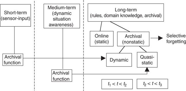
FIGURE 24.3
Possible implementation strategy for temporally sensitive spatial data.
Rather than reviewing the large body of literature associated with spatial database design and spatiotemporal reasoning, this chapter focuses on a conceptual level view of the problem. Figure 24.2 offers a temporal sensitivity taxonomy for spatial data, and Figure 24.3 maps the three classes of temporal sensitivity to a human memory metaphor. Later discussions will focus on a potential implementation strategy based on Figure 24.3.
On the surface, treating time as an independent variable (or dimension) seems quite reasonable. However, treating time as an independent variable requires the spatial dimensions of a spatial–temporal representation to become the dependent dimensions. Because we seek a representation that supports object-oriented reasoning, and objects are typically associated with physical or aggregate entities that exist within a 2D or 3D world, such an arrangement seems unworkable. In tactical data fusion applications, the spatial attributes of physical objects (e.g., location, shape, velocity, and path) represent key problem dimensions, with time generally playing a subordinate role.

FIGURE 24.4
Two-dimensional depiction of data set showing the spatial relationships between the various features.
The benefits of employing a true n-dimensional spatial data structure* and therefore treating time as a dependent variable can be illustrated by the following simple example. Suppose an existing fusion database contains the temporally sorted entity locations:
(xa, ya, ta) = (1, 1, 1)
(xc, yc, tc) = (3, 3, 5)
(xb, yb, tb) = (5, 2, 10)
Assume a new sensor report, indicating a target detection at (xd, yd, td) = (3, 1.5, 5), must be fused with the existing data set. Direct comparison of this new report with the existing database suggests that query point d is near point c (i.e., tc = td) and not near either point a or b. If the database was sorted by all three dimensions, with the y-coordinate selected as the primary index dimension, point d would appear to be near point a and not near either point b or c. Suppose that the detections occurring at points a and b represent successive detections of the same entity (i.e., the endpoints of a track segment). As illustrated in Figure 24.4, which depicts the existing data set and all new detections in a true 2D spatial representation (rather than a list-oriented, tuple-based representation), query point d is readily discovered to be spatially distant from all three points, but spatially close to the line segment a–b.
To accommodate the temporal dimension, the distance between (xd, yd) and the interpolated target position along the line segment a–b (at time td) can be readily computed. If the target under track is known to be a wheeled vehicle moving along a road network, data associations can be based on a road-constrained trajectory, rather than a linear trajectory.
Although target reports typically occur at discrete times (e.g., at radar revisit rates), the trajectory of physical objects is a continuous function in both space and time. Despite the fact that the closest line segment to an arbitrary point in space can be derived from tuple-based data, much more efficient data retrieval is possible if all spatial features are explicitly represented within the database. Thus, by employing a time-coded, explicit spatial representation (and not just preserving line segment endpoints), a database can effectively support a search along continuous dimensions in both space and time. With such a representation, candidate track segments can be found through highly localized (true 2D) spatial searches about point d.
Representing moving targets by continuous, time-referenced spatially organized trajectories not only matches the characteristics of physical phenomenon, but also supports highly effective database search dimensions. Equally important, such representations preserve spatial relationships between dynamic objects and other static and dynamic spatially organized database entities. Thus, there exist multiple justifications for subordinating temporal indexing to spatial indexing.
Both semantic and spatial reasoning are intrinsically hierarchical. Semantic object reasoning relies heavily on explicitly represented object hierarchies; similarly, spatial reasoning can benefit from multiple-resolution spatial representations. Time is a monotonically increasing function; therefore, temporal phenomena possess a natural sequential ordering, which can be treated as a specialized hierarchical representation. These considerations attest to the appropriateness of subordinating hierarchical reasoning to both semantic and spatial reasoning and, in turn, subordinating temporal reasoning to hierarchical reasoning.
Figure 24.5 depicts the hierarchical relationship that exists between the three reasoning classes. At the highest level of abstraction, reasoning can be treated as either spatial or semantic (nonspatial). Each of these reasoning classes can be handled using either hierarchical or nonhierarchical approaches. Hierarchical spatial reasoning employs multiple-resolution spatial representations, and hierarchical nonspatial reasoning uses tree-structured semantic representations. Each of these classes, in turn, may or may not be temporally sensitive.
If we refer to temporal reasoning as dynamic reasoning and nontemporal reasoning as static reasoning, there exist four classes of spatial reasoning and four classes of nonspatial reasoning: (1) dynamic, hierarchical; (2) static, hierarchical; (3) dynamic, nonhierarchical; and (4) static, nonhierarchical. To effectively support data fusion automation, a database must accommodate each of these reasoning classes. Because nonhierarchical reasoning is a special case of hierarchical reasoning, and static reasoning is a special case of dynamic reasoning, data fusion applications are adequately served by a DBMS that provides dynamic, hierarchical spatial representations and dynamic, hierarchical semantic representations. Thus, supporting these two key reasoning classes represents the primary database design criterion.

FIGURE 24.5
Taxonomy of the three principal reasoning classes.
24.4 Database Design Criteria
This section addresses key database design criteria to support advanced algorithm development. Data representation can have a profound impact on algorithm development. The preceding discussion regarding spatial, temporal, and hierarchical reasoning highlighted the benefit of representations that provide natural search dimensions and preserve significant relationships among domain objects. In addition to supporting key database operations, such as search efficiency, intuitive data representations facilitate the development of sophisticated algorithms that emulate the top-down reasoning process of human analysts.
24.4.1 Intuitive Algorithm Development
In analyzing personnel data, for example, table-based representations are much more natural (and useful) than tree-based data structures. Hierarchical data structures are generally more appropriate for representing the organization of a large company than a spatially organized representation. Raster representations of imagery tend to support more intuitive image processing algorithms than do vector-based representations of point, line, and region boundary-based features.
The development of sophisticated machine-based reasoning benefits from full integration of both the semantic and the spatial data representations, as well as integration among multiple representations of a given data type. For example, a river possesses both semantic attributes (class, nominal width, and flow-rate) and spatial attributes (beginning location, ending location, shape description, and depth profile). At a reasonably low resolution, a river’s shape might be best represented as a lineal feature; at a higher resolution, a region-based representation is likely more appropriate.
24.4.2 Efficient Algorithm Performance
For algorithms that require large supporting databases, data representation form can significantly affect algorithm performance efficiency. For business applications that demand access to massive table-based data sets, the relational data model supports more efficient algorithm performance than a semantic network model. Two-dimensional template matching algorithm efficiency tends to be higher if true 2D (map-like) spatial representations are used rather than vector-based data structures. Multiple level-of-abstraction semantic representations and multiple-resolution spatial representations tend to support more efficient problem solving than do nonhierarchical representations.
24.4.3 Data Representation Accuracy
In general, data representation accuracy must be adequate to support the widest possible range of data fusion applications. For finite resolution spatially organized representations, accuracy depends on the data sampling method. In general, data sampling can be either uniform or nonuniform. Uniformly sampled spatial data are typically maintained as integers, whereas nonuniformly sampled spatial data are typically represented using floating-point numbers. Although the pixel-based representation of a region boundary is an integer-based representation, a vector-based representation of the same boundary maintains the vertices of the piecewise linear approximation of the boundary as a floating-point list. For a given memory size, nonuniformly sampled representations tend to provide higher accuracy than uniformly sampled representations.
24.4.4 Database Performance Efficiency
Algorithm performance efficiency relies on the six key database efficiency classes described in the following paragraphs.
24.4.4.1 Storage Efficiency
Storage efficiency refers to the relative storage requirements among alternative data representations. Figure 24.6 depicts two similar polygons and their associated vector, raster, pixel boundary, and quadtree representations. With a raster representation (Figures 24.6c and 24.6d), A/∆2 nodes are required to store the region, where A is the area of the region, and ∆ is the spatial width of a (square) resolution cell (or pixel). Accurate replication of the region shown in Figure 24.6a requires a resolution cell size four times smaller than that required to replicate the region in Figure 24.6b. Because the pixel boundary representation (Figures 24.6e and 24.6f) maintains only the boundary nodes of the region, the required node count is proportional to P/∆, where P is the perimeter of the region. For fixed ∆, the ratio of the node count for the raster representation relative to the pixel boundary representation is A/(∆P). Although a quadtree representation (Figures 24.6g and 24.6h) stores both the region boundary and its interior, the required node count, for large regions, is proportional to the region perimeter rather than its area.1 Thus, for grid-based spatial decompositions, the region node count depends on the maximum resolution cell size and the overall size of the region (either its area or perimeter).

FIGURE 24.6
Storage requirements for four spatial data representations of two similarly shaped regions.
Whereas storage requirements for grid-based representations tend to be dependent on the size of the region, storage requirements for nonuniform decompositions are sensitive to the small-scale feature details. Consequently, for nonuniform representations, no simple relationship exists between a region’s size and its storage requirements. For example, two regions of the same physical size possessing nearly identical uniform decomposition storage requirements might have dramatically different storage requirements under a nonuniform decomposition representation. Vector-based polygon representations are perhaps the most common nonuniform decomposition. In general, when the level of detail in the region boundary is high, the polygon tuple count will be high; when the level of detail is low, few vertices are required to represent the boundary accurately. Because the level of detail of the boundaries in both Figures 24.6a and 24.6b are identical, both require the same number of vertices. In general, for a given accuracy, nonuniform decompositions have significantly lower storage requirements than uniform decompositions.
24.4.4.2 Search Efficiency
Achieving search efficiency requires effective control of the search space size for the range of typical database queries. In general, search efficiency can be improved by storing or indexing data sets along effective search dimensions. For example, for vector-represented spatial data sets, associating a bounding box (i.e., vertices of the rectangle that forms the smallest outer boundary of a line or region) with the representation provides a simple indexing scheme that affords significant search reduction potential. Many kinds of data possess natural representation forms that, if preserved, facilitate the search. 2D representations that preserve the essential character of maps, images, and topographic information permit direct access to data along very natural 2D search dimensions. Multiple-resolution spatial representations potentially support highly efficient top-down spatial search and reasoning.
24.4.4.3 Overhead Efficiency
Database overhead efficiency includes both indexing efficiency and data maintenance efficiency. Indexing efficiency refers to the cost of creating data set indices, whereas data maintenance efficiency refers to the efficiency of re-indexing and reorganization operations, including tree-balancing required following data insertions or deletions. Because natural data representations do not require separate indexing structures, such representations tend to support overhead efficiency. Although relatively insignificant for static databases, database maintenance efficiency can become a significant factor in highly dynamic data sets.
24.4.4.4 Association Efficiency
Association efficiency refers to the efficient determination of relationships among data sets (e.g., inclusion, proximity). Natural data representations tend to significantly enhance association efficiency over vector-based spatial representations because they tend to preserve the inherent organizational characteristics of data. Although relational database tables can be joined (via a static, single-dimension explicit key), the basic relational model does not support efficient data set association for data that possess correlated attributes (e.g., combined spatial and temporal proximity).
24.4.4.5 Complex Query Efficiency
Complex query efficiency includes both set operation efficiency and complex clause evaluation efficiency. Set operation efficiency demands efficient Boolean and fuzzy set operations among point, line, and region features. Complex clause evaluation efficiency requires query optimization for compound query clauses, including those with mixed spatial and semantic constraints.
24.4.4.6 Implementation Efficiency
Implementation efficiency is enhanced by a database architecture and associated data structures that support the effective distribution of data, processing, and control. Figure 24.7 summarizes these 12 key design considerations.
24.4.5 Spatial Data Representation Characteristics
Many spatial data structures and numerous variants exist. The taxonomy depicted in Figure 24.8 provides an organizational structure that is useful for comparing and contrasting spatial data structures. At the highest level of abstraction, sampled representations of 2D space can employ either uniform (regular) or nonuniform (nonregular) decompositions. Uniform decompositions generate data-independent representations, whereas nonuniform decompositions produce data-dependent representations.
With certain exceptions (e.g., fractal-like data), low-resolution representations of spatial features tend to be uniformly distributed and high-resolution representations of spatial data tend to be nonuniformly distributed. Consequently, uniform decompositions tend to be most appropriate for storing relatively low-resolution spatial representations, as well as supporting both data registration and efficient spatial indexing. Conversely, nonuniform decompositions support memory-efficient high-resolution spatial data representations.

FIGURE 24.7
High-level summary of the database design criteria.

FIGURE 24.8
Spatial data structure taxonomies with the recommended representation branches outlined in bold gray lines.
Hierarchical decompositions of 2D spatial data support the continuum from highly global to highly local spatial reasoning. Global analysis typically begins with relatively low-resolution data representations and relatively global constraints. The resulting analysis products are then progressively refined through higher-resolution analysis and the application of successively more local constraints. For example, a U.S. Interstate road map provides a low-resolution representation that supports the first stage of a route-planning strategy. Once a coarse resolution plan is established, various state, county, and city maps can be used to refine appropriate portions of the plan to support excursions from the Interstate highway to visit tourist attractions or to find lodging and restaurants. Humans routinely employ such top-down reasoning, permitting relatively global (often near-optimal) solutions to a wide range of complex tasks.
Data decompositions that preserve the inherent 2D character of spatial data are defined to be 2D data structures. 2D data structures provide natural spatial search dimensions, eliminating the need to maintain separate search indices. In addition, such representations preserve Euclidean distance metrics and other spatial relationships. Thus, a raster representation is considered a 2D data structure, whereas tuple-based representations of lines and region boundaries are non-2D data structures.
Explicit data representations literally depict a set of data, whereas implicit data representations maintain information that permits reconstruction of the data set. Thus, a raster representation is an explicit data representation because it explicitly depicts line and region features. A vector representation, which maintains only the endpoint pairs of piecewise continuous lines and region boundaries, is considered an implicit representation. In general, implicit representations tend to be more memory-efficient than explicit representations.
Specific feature spatial representations maintain individual point, line, and region features, and composite feature spatial representations store the presence or absence of multiple features. Specific spatial representations are most effective for performing spatial operations with respect to individual features; composite representations are most effective for representing classes of spatial features.
Areal-based representations maintain a region’s boundary and interior. Nonareal-based representations explicitly store only a region’s boundary. Boolean set operations among 2D spatially organized data sets inherently involve both boundaries and region interiors. As a result, areal-based representations tend to support more efficient set operation generation than nonareal-based representations among all classes of spatial features.
Data that are both regular and hierarchical support efficient tree-oriented spatial search. Regular decompositions utilize a fixed grid size at each decomposition level and provide a fixed resolution relationship between levels, enabling registered data sets to be readily associated at all resolution levels. Registered data representations that are both regular and areal-based support efficient set operations among all classes of 2D spatial features. Because raster representations are both regular and areal-based, set intersection generation requires only simple Boolean AND operations between respective raster cells. Similarly, set union can be computed as the Boolean OR between the respective cells.
Spatial representations that are both regular and 2D preserve spatial adjacency among all classes of spatial features. They employ a data-independent, regular decomposition and, therefore, do not require extensive database rebuilding operations following insertions and deletions. In addition, because no separate spatial index is required, re-indexing operations are unnecessary. Spatially local changes tend to have highly localized effects on the representation; as a result, spatial decompositions that are both regular and 2D are relatively dynamic data structures. Consequently, database maintenance efficiency is generally enhanced by regular 2D spatial representations.
Data fusion involves the composition of both dynamic (sensor data, existing fusion products) and static (tables of equipment, natural and cultural features) data sets; consequently, data fusion algorithm efficiency is enhanced by employing compatible data representation forms for both dynamic and static data. For example, suppose the (static) road network was maintained in a nonregular vector-based representation, whereas the (dynamic) target track file database was maintained in a regular 2D data structure. The disparate nature of the representations would make the fusion of these data sets both cumbersome and inefficient. Thus, maintaining static and dynamic information with identical spatial data structures potentially enhances both database association efficiency and maintenance efficiency.
Spatial representations that are explicit, regular, areal, and 2D support efficient set operation generation, offer natural search dimensions for fully registered spatial data, and represent relatively dynamic data structures. Because they possess key characteristics of analog 2D spatial representations (e.g., paper maps and images), the representations are defined to be true 2D spatial representations. Spatial representations possessing one or more of the following properties violate the requirements of true 2D spatial representations:
Spatial data is not stored along 2D search dimensions (i.e., spatial data stored as list or table-based representations).
Region representations are nonareal-based (i.e., bounding polygons).
Nonregular decompositions are employed (e.g., vector representations and R-trees).
True 2D spatial representations tend to support both intuitive algorithm development and efficient spatial reasoning. Such representations preserve key 2D spatial relationships, thereby supporting highly intuitive spatial search operations (e.g., northwest of point A, beyond the city limits, or inside a staging area). Because grid-based representations store both the boundary and the interior of a region, intersection and union operations among such data can be generated using straightforward cell-by-cell operations. The associated computational requirements scale linearly with data set size independent of the complexity of the region data sets (e.g., embedded holes or multiple disjoint regions). Conversely, set operation generation among regions based on non-true-2D spatial representations tend to require combinatorial computational requirements.
Computational geometry approaches to set intersection generation require the determination of all line segment intersection points; therefore, computational complexity is of the order m × n, where m and n are the number of vertices associated with the two polygons. When one or both regions contain embedded holes, dramatic increases in computational complexity can result. For analysis and fusion algorithms that rely on set intersections among large complex regions, algorithm performance can be adversely impacted. Although the use of bounding rectangles (bounding boxes) can significantly enhance search and problem-solving efficiency for vector-represented spatial features, they provide limited benefit for multiple-connected regions, extended lineal features (e.g., roads, rivers, and topographic contour lines), and directional and proximity-based searches.
Specific spatial representations that are explicit, regular, areal, 2D, and hierarchical (or hierarchical true 2D) support highly efficient top-down spatial search and top-down areal-based set operations among specific spatial features. With a quadtree-based region representation, for example, set intersection can be performed using an efficient top-down, multiple-resolution process that capitalizes on two key characteristics of Boolean set operations. First, the intersection product is a proper subset of the smallest region being intersected. Second, the intersection product is both commutative and associative and, therefore, independent of the order in which the regions are composed. Thus, rather than exhaustively ANDing all nodes in all regions, intersection generation can be reformulated as a search problem where the smallest region is selected as a variable resolution spatial search window for interrogating the representation of the next larger region.1 Nodes in the second smallest region that are determined to be within this search window are known to be in the intersection product. Consequently, the balance of the nodes in the larger region need not be tested.
If three or more regions are intersected, the product that results from the previous intersection product becomes the search window for interrogating the next larger region. Consequently, whereas the computational complexity of polygon intersection is a function of the product of the number of vertices in each polygon, the computational complexity for region intersection using a regular grid-based representation is related to the number of tuples that occur within cells of the physically smallest region. Composite spatial representations that are explicit, regular, areal, 2D, and hierarchical support efficient top-down spatial search among classes of spatial features.
Based on the relationships between spatial data decomposition classes and key database efficiency classes, a number of generalizations can be formulated:
Hierarchical, true 2D spatial representations support the development of highly intuitive algorithms.
For tasks that require relatively low-resolution spatial reasoning, algorithm efficiency is enhanced by hierarchical, true 2D spatial representations.
Implicit, nonregular spatial representations support representation accuracy.
Specific spatial representations are most appropriate for reasoning about specific spatial features; conversely, composite spatial representations are preferable for reasoning about classes of spatial features. For example, a true 2D composite road network representation would support more efficient determination of the closest road to a given point in space than a representation maintaining individual named roads. With the latter representation, a sizable portion of the road database would have to be interrogated.
Finite resolution data decompositions that are implicit, nonregular, nonhierarchical, nonareal, and non-2D tend to be highly storage-efficient.
Spatial indexing efficiency is enhanced by hierarchical, true 2D representations that support natural, top-down search dimensions.
Spatially local changes require only relatively local changes to the underlying representation; therefore, database maintenance efficiency is enhanced by regular, dynamic, 2D spatial representations.
For individual spatial features, database search efficiency is enhanced by spatial representations that are specific, hierarchical, and true 2D, and that support distributed search.
Search efficiency for classes of spatial features is enhanced by composite hierarchical spatial feature representations.
True 2D spatial representations preserve spatial relationships among data sets; therefore, for individual spatial features, database association efficiency is enhanced by hierarchical true 2D spatial representations of specific spatial features. For classes of spatial features, association efficiency is enhanced by hierarchical, true 2D composite feature representations.
For specific spatial features, complex query efficiency is enhanced by hierarchical, true 2D representations of individual features; for classes of spatial features, complex query efficiency is enhanced by hierarchical, composite, true 2D spatial representations.
Finally, database implementation efficiency is enhanced by data structures that support the distribution of data, processing, and control.
These general observations are summarized in Table 24.1.
24.4.6 Database Design Tradeoffs
Object-oriented reasoning potentially supports the construction of robust, context-sensitive fusion algorithms, enabling data fusion automation to benefit from the development of an effective OODBMS. This section explores design tradeoffs for an object-oriented database that seek to achieve an effective compromise among the algorithm support and database efficiency issues listed in Table 24.1. As previously discussed, the principal database design requirement is support for dynamic, hierarchical spatial reasoning and dynamic, hierarchical semantic reasoning. Consequently, an optimal database must provide data structures that facilitate storage and access to both temporally and hierarchically organized spatial and nonspatial information.
TABLE 24.1
Spatial Representation Attributes Supporting Nine Spatial Database Requirements

Nonspatial (or semantic) declarative knowledge can be represented as n-tuples, arrays, tables, transfer functions, frames, trees, and graphs. Modern semantic object databases provide effective support to complex, multiple level-of-abstraction problems that (1) possess extensive parent–child relationships, (2) benefit from problem decomposition, or (3) demand global solutions. Because object-oriented representations permit the use of very general internal data structures, and the associated reasoning paradigm fully embraces hierarchical representations at the semantic object level, conventional object databases intrinsically support hierarchical semantic reasoning. Semantic objects can be considered relatively dynamic data structures because temporal changes associated with a specific object tend to affect only that object or closely related objects.
The character and capabilities of a spatial object database are analogous to those of a semantic object database. A spatial object database must support top-down, multiple level-of-abstraction (i.e., multiple resolution) reasoning with respect to classes of spatial objects, as well as permit efficient reasoning with specific spatial objects. Just as the semantic object paradigm requires an explicitly represented semantic object hierarchy, a spatial object database requires an equivalent spatial object hierarchy. Finally, just as specific entities in conventional semantic object databases possess individual semantic object representations, specific spatial objects require individual spatial object representations.
24.5 Object Representation of Space
Consider the query:
Determine the class-1 road closest to query point (x1, y1).
In a database that maintains only implicit representations of individual spatial features, this feature-class query could potentially require the interrogation of all class-1 road representations. Just as a hierarchical representation of semantic objects permits efficient class-oriented queries, a hierarchical representation of space supports efficient queries with respect to classes of spatial objects. At the highest level of abstraction, an object representation of space consists of a single object that characterizes the entire area of interest (Asia, a single map sheet, a division’s area of interest). At each successively lower level of the spatial object hierarchy, space is decomposed into progressively smaller regions that identify spatial objects (specific entities or entity classes) associated with that region. Just as higher-order semantic objects possess more general properties than their offspring, higher-order object representations of space characterize the general properties of 2D space.
Based on the principles outlined in the last section, an object representation of 2D space must satisfy the properties summarized in Table 24.2. As previously mentioned, a true 2D spatial representation possesses the first five characteristics listed in Table 24.2. With the addition of the sixth property, the spatial object hierarchy provides a uniform hierarchical spatial representation for classes of point, line, and region features. The pyramid data structure fully satisfies these first six properties. Because multiple classes of spatial objects (e.g., roads, waterways, and soil type) can be maintained within each cell, a pyramid representation is well suited to maintain a composite feature representation. In a pyramid representation, all the following are true:
Spatially local changes require only relatively local changes to the data structure.
Limited re-indexing is required following updates.
Extensive tree-balancing operations are not required following insertions or deletions.
TABLE 24.2
Key Representation Characteristics Required by the Three Distinct Spatial Data Representation Classes

As a result, the pyramid is a relatively dynamic data structure. In addition, the hierarchical and grid-based character of the pyramid data structure enables it to readily accommodate data distribution. Therefore, a pyramid data structure fully satisfies all nine requirements for an object representation of 2D space.
24.5.1 Low-Resolution Spatial Representation
As summarized in Table 24.2, an effective low-resolution spatial representation must possess 10 key properties. With the exception of the composite feature representation property, the low-resolution spatial representation requirements are identical to those of the object representation of 2D space. Whereas a composite-feature-based representation supports efficient spatial search with respect to classes of spatial features, a specific feature-based representation supports effective search and manipulation of specific point, line, and region features. A regular region quadtree possesses all of the properties presented in Table 24.2, column 3.
24.5.2 High-Resolution Spatial Representation
An effective high-resolution spatial representation must possess the 10 properties indicated in the last column of Table 24.2. Vector-based spatial representations clearly meet the first four criteria. Because they use nonhierarchical representations of specific features and employ implicit piecewise linear representations of lines and region boundaries, vector representations also satisfy properties 5–7. Changes to a feature require a modification of the property list of a single feature; therefore, vector representations tend to be relatively dynamic data structures. A representation of individual features is self-contained, so vector representations can be processed in a highly distributed manner. Finally, vector-based representations inherently provide high precision. Thus, vector-based representations satisfy all of the requirements of the high-resolution spatial representation.

FIGURE 24.9
Quadtree-indexed vector spatial representation for points, lines, and regions.
24.5.3 Hybrid Spatial Feature Representation
Traditionally, spatial database design has involved the selection of either a single spatial data structure or two or more alternative, but substantially independent, data structures (e.g., vector and quadtree). Because of the additional degrees of freedom it adds to the design process, the use of a hybrid spatial representation offers the potential for achieving a near-optimal compromise across the spectrum of design requirements. Perhaps the most straightforward design approach for such a hybrid data structure is to directly integrate a multiple-resolution, low-resolution spatial representation and a memory-efficient, high-resolution spatial representation.
As indicated in Figure 24.9, the quadtree data structure can form the basis of an effective hybrid data structure, serving the role of both a low-resolution spatial data representation and an efficient spatial index into high-accuracy vector representations of point, line, and region boundaries. Table 24.3 offers a coarse-grain evaluation of the effectiveness of the vector, raster, pixel boundary, region quadtree, and the recommended hybrid spatial representation based on the database design criteria. Table 24.4 summarizes the key characteristics of the recommended spatial object representation and demonstrates that it addresses the full spectrum of spatial data design issues.
24.6 Integrated Spatial/Nonspatial Data Representation
To effectively support data fusion applications, spatial and nonspatial data classes must be fully integrated. Figure 24.10 depicts a high-level view of the resultant semantic/spatial database kernel depicting both explicit and implicit links between the various data structures. Because a pyramid data structure can be viewed as a complete quadtree, the pyramid and the low-resolution spatial representation offer a unified structure, with the latter effectively an extension to the former. Therefore, the quadtree data structure serves as the link between the pyramid and the individual spatial feature representations and provides a hierarchical spatial index to high-resolution vector-represented point, line, and region features.
TABLE 24.3
Comparison of Spatial Data Representations Based on Their Ability to Support Database Design Criteria

TABLE 24.4
Summary Characteristics of the Three Spatial Representation Classes

The integrated spatial and semantic object representation permits efficient top-down search for domain objects based on a combination of semantic and spatial constraints. The fully integrated data structures support efficient and effective manipulation of spatial and nonspatial relations, and the computation of spatial and semantic distance metrics among domain objects. The quadtree-indexed data structure preserves the precision of the highest-fidelity spatial data without compromising the memory efficiency of the overall system.

FIGURE 24.10
High-level view of the integrated semantic/spatial object database.
24.7 Sample Application
This section illustrates key benefits of the proposed database system design by applying the concepts to a simple, easily visualized path-planning application. Humans routinely plan simple tasks in a nearly subconscious manner (e.g., walking from one room to another and picking up a glass of water); however, other tasks require considerable deliberation. Consider, for instance, planning an automobile trip from Washington, District of Columbia to Portland, Oregon. Adding constraints to the problem, such as stops at nearby national parks and other attractions along the way, can significantly complicate the task of generating an optimal plan. One approach to planning such a trip would be to accumulate all the county road maps through which such a route might pass; however, the amount of data would be overwhelming. The task would be much less daunting if the planner first acquired a map of the U.S. Interstate highway system used this map to select a coarse resolution plan. Then, a small collection of state maps would probably suffice for planning routes to specific attractions located some distance from an interstate highway. Finally, for locating a friend’s residence, a particular historical landmark, or some other point of interest, detailed county or even city maps could be used to refine the details of the overall plan.
Clearly, the top-down path development approach is both more natural and much more efficient than a single level-of-abstraction approach, exploiting the continuum from global to highly local objectives and evaluation metrics. Given a time- and resource-constrained vacation, the relative importance of competing objectives might need to be weighted to generate something close to an optimal plan.
In path planning, as with virtually all decision making, effective evaluation criteria are needed to select among large numbers of candidate solutions. Path selection metrics could be as simple as seeking to minimize the overall path length, minimize travel time, or maximize travel speed. However, the planner may want to minimize or maximize a weighted combination of several individual metrics or to apply fuzzier (more subjective) measures of performance. Whereas crisp metrics can be treated as absolute metrics (e.g., the shortest path length or the fastest speed), fuzzy metrics are most appropriate for representing relative metrics or constraints (e.g., selecting a moderately scenic route that is not much longer than the shortest route). In addition to selection criteria, various problem constraints could be appropriate at the different levels of the planning process. These might include regular stops for fuel, meals, and nightly motel stays.
In addition to developing effective a priori plans, real-world tasks often require the ability to perform real-time replanning. Replanning can span the spectrum from global modifications to highly local changes. As an illustration of the latter, suppose a detailed plan called for travel in the right-hand lane of Route 32, a four-lane divided highway. During plan execution, an accident is encountered blocking further movement in the rightmost lane requiring the initial plan to be locally adjusted to avoid this impasse. More global modifications would be required if, before reaching Route 32, the driver learned of a recent water main break that was expected to keep the road closed to traffic the entire day.
In general, top-down planning begins by establishing a coarse-grain skeletal solution, which is then recursively refined to the appropriate level of detail. Multiple level-of-abstraction planning tends to minimize the size of both the search and decision spaces, making it highly effective. Based on both its efficacy and efficiency, top-down planning readily accommodates replanning, a critical component in complex, dynamic problem domains.
24.7.1 Problem-Solving Approach
This section outlines a hierarchical path-planning algorithm that seeks to develop one or more routes between two selected locations for a wheeled military vehicle capable of both on-road and off-road movement. Rather than seeking a mathematically optimal solution, we strive for a near-optimal global solution by emulating a human-oriented approach to path selection and evaluation.
In general, path selection is potentially sensitive to a wide range of geographical features (i.e., terrain, elevation changes, soil type, surface roughness, and vegetation), environmental features (i.e., temperature, time of day, precipitation rate, visibility, snow depth, and wind speed), and cultural features (i.e., roads, bridges, the location of supply caches, and cities). Ordering the applicable domain constraints from the most to the least significant effectively treats path development as a top-down, constraint-satisfaction task.
In general, achieving high quality global solutions requires that global constraints be applied before more local constraints. Thus, in stage 1 (the highest level of abstraction), path development focuses on route development, considering only extended barriers to ground travel. Extended barriers are those cultural and man-made features that cannot be readily circumnavigated. As a natural consequence, they tend to have a more profound impact on route selection than smaller-scale features. Examples of extended features include rivers, canyons, neutral zones, ridges, and the Great Wall in China. Thus, in terms of the supporting database, first-stage analysis involves searching for extended barriers that lie between the path’s start and goal state.
If an extended barrier is discovered, candidate barrier-crossing locations (e.g., bridges or fording locations for a river or passes for a mountain range) must be sought. One or more of these barrier-crossing sites must be selected as candidate high-level path subgoals. As with all stages of the analysis, an evaluation metric is required to either prune or rank candidate subgoals. For example, the selected metric might retain the n closest bridges possessing adequate weight-carrying capacity. For each subgoal that satisfies the selection metric, the high-level barrier-crossing strategy is reapplied, searching for extended barriers and locating candidate barrier-crossing options until the final goal state is reached. The product of stage 1 analysis is a set of coarse resolution candidate paths represented as a set of subgoals that satisfy the high-level path evaluation metrics and global domain constraints.
Because the route is planned for a wheeled vehicle, the existing road network has the next most significant impact on route selection. Thus, in stage 2, road connectivity is established between all subgoal pairs identified in stage 1. For example, the shortest road path or the shortest m road paths are generated for those subgoals discovered to be on or near a road. When the subgoal is not near a road or when path evaluation indicates that all candidate paths provide only low-confidence solutions, overland travel between the subgoals would be indicated. Upon completion of stage 2 analysis, the coarse resolution path sets that have been developed during stage 1 will be refined with the appropriate road-following segments.
In stage 3, overland paths are developed between all subgoal pairs not already linked by high-confidence, road-following paths. Whereas extended barriers were associated with the most global constraints on mobility, nonextended barriers (e.g., hills, small lakes, drainage ditches, fenced fields, or forests) represent the most significant mobility constraints for overland travel. Ordering relevant nonextended barriers from stronger constraints (i.e., larger barriers and no-go regions) to weaker constraints (i.e., smaller barriers and slow-go regions) will extend the top-down analysis process. At each successive level of refinement, a selection metric, sensitive to progressively more local path evaluation constraints, is applied to the candidate path sets. The path refinement process terminates when one or more candidate paths have been generated that satisfy all path evaluation constraints. Individual paths are then rank-ordered against selected evaluation metrics.
Whereas traditional path development algorithms generate plans based on brute force optimization by minimizing path resistance or other similar metric, the hierarchical constraint-satisfaction-based approach just outlined emulates a more human-like approach to path development. Rather than using simple, single level-of-abstraction evaluation metrics (path resistance minimization), the proposed approach supports more powerful reasoning, including concatenated metrics (e.g., maximal concealment from one or more vantage points plus minimal travel time to a goal state). A path that meets both of these requirements might consist of a set of road segments not visible from specified vantage points, as well as high-mobility off-road path segments for those sections of the roadway that are visible from those vantage points. Hierarchical constraint-based reasoning captures the character of human problem-solving approaches, achieving the spectrum from global to more local subgoals, producing intuitively satisfying solutions. In addition, top-down, recursive refinement tends to be more efficient than approaches that attempt to directly generate high-resolution solutions.
24.7.2 Detailed Example
This section uses a detailed example of the top-down path-planning process to illustrate the potential benefits of the integrated semantic and spatial database discussed in Section 24.6. Because the database provides both natural and efficient access to both hierarchical semantic information and multiple-resolution spatial data, it is well suited to problems that are best treated at multiple levels of abstraction. The tight integration between semantic and spatial representation allows effective control of both the search space and the solution set size.
The posed problem is to determine one or more good routes for a wheeled vehicle from the start to the goal state depicted in Figure 24.11. Stage 1 begins by performing a spatially anchored search (i.e., anchored by both the start and goal states) for extended mobility barriers associated with both the cultural and the geographic feature database. As shown in Figure 24.12, the highest level-of-abstraction representation of the object representation of space (i.e., the top-level of the pyramid) indicates that a river, which represents an extended ground-mobility barrier, exists in the vicinity of both the start and the goal states. At this level of abstraction, it cannot be determined whether the extended barrier lies between the two points.
The pyramid data structure supports highly focused, top-down searching to determine whether ground travel between the start and the goal states is blocked by a river. At the next higher-resolution level, however, ambiguity remains. Finally, at the third level of the pyramid, it can be confirmed that a river lies between the start and the goal states. Therefore, an efficient, global path strategy can be pursued that requires breaching the identified barrier. Consequently, bridges, suitable fording locations, or bridging operations become candidate subgoals.

FIGURE 24.11
Domain mobility map for path development algorithm.

FIGURE 24.12
Top-down multiple-resolution spatial search, from the start toward the goal node, reveals the existence of a river barrier.
If, however, no extended barrier had been discovered in the cells shared by the start and the goal states (or in any intervening cells) at the outset of stage 1 analysis, processing would terminate without generating any intervening subgoals. In this case, stage 1 analysis would indicate that a direct path to the goal is feasible.
Whereas conventional path-planning algorithms operate strictly in the spatial domain, a flexible top-down path-planning algorithm supported by an effectively integrated semantic and spatial database can operate across both the semantic and the spatial domains. For example, suppose nearby bridges are selected as the primary subgoals. Rather than perform spatial search, direct search of the semantic object (River 1) could determine nearby bridges. Figure 24.13 depicts attributes associated with that semantic object, including the location of a number of bridges that cross the river. To simplify the example, only the closest bridge (Bridge 1) will be selected as a candidate subgoal (denoted SG1,1). Although this bridge could have been located via spatial search in both directions along the river (from the point at which a line from the start to the goal state intersects River 1), a semantic-based search is more efficient.
To determine if one or more extended barriers lie between SG1,1 and the goal state, a spatial search is reinitiated from the subgoal in the direction of the goal state. High-level spatial search within the pyramid data structure reveals another potential river barrier. Top-down spatial search once again verifies the existence of a second extended barrier (River 2). Just as before, the closest bridging location, denoted as SG1,2, is identified by evaluating the bridge locations maintained by the semantic object (River 2). Spatial search from Bridge 2 toward the goal state reveals no extended barriers that would interfere with ground travel between the SG1,2 and the goal state.

FIGURE 24.13
Semantic object database for the path development algorithm.

FIGURE 24.14
Subgoals associated with all three stages of the path development algorithm.
As depicted in Figure 24.14, the first stage of the path development algorithm generates a single path consisting of the three subgoal pairs (start, SG1,1), (SG1,1, SG1,2), and (SG1,2, goal) satisfying the global objective of reaching the goal state by breaching all extended barriers. Thus, at the conclusion of stage 1, the primary alternatives to path flow have been identified.
In stage 2, road segments connecting adjacent subgoals that are on or near the road network must be identified. The semantic object representation of the bridges identified as subgoals during the stage 1 analysis also identify their road association; therefore, a road network solution potentially exists for the subgoal pair (SG1,1, SG1,2). Algorithms are widely available for efficiently generating minimum distance paths within a road network. As a result of this analysis, the appropriate segments of Road 1 and Road 2 are identified as members of the candidate solution set (shown in bold lines in Figure 24.14).
Next, the paths between the start state and SG1,1 are investigated. SG1,1 is known to be on a road and the start state is not; therefore, determining whether the start state is near a road is the next objective. Suppose the assessment is based on the fuzzy qualifier near shown in as Figure 24.15. Because the detailed spatial relations between features cannot be economically maintained with a semantic representation, spatial search must be used. Based on the top-down, multiple-resolution object representation of space, a road is determined to exist within the vicinity of the start node. A top-down spatially localized search within the pyramid efficiently reveals the closest road segment to the start node. Computing the Euclidean distance from that segment to the start node, the start node is determined to be near a road with degree of membership 0.8.
Because the start node has been determined to be near a road, in addition to direct overland travel toward Bridge 1 (start, SG1,1), an alternative route exists based on overland travel to the nearest road (subgoal SG2,1) followed by road travel to Bridge 1 (SG2,1, SG1,1). Although a spectrum of variants exists between direct travel to the bridge and direct travel to the closest road segment, at this level of abstraction only the primary alternatives must be identified. Repeating the analysis for the path segment (SG1,2, goal), the goal node is determined to be not near any road. Consequently, overland route travel is required for the final leg of the route.
In stage 3, all existing nonroad path segments are refined based on more local evaluation criteria and mobility constraints. First, large barriers, such as lakes, marshes, and forests, are considered. Straight-line search from the start node to SG1,1 reveals the existence of a large lake. Because circumnavigation of the lake is required, two subgoals are generated (SG3,1 and SG3,2) as shown in Figure 24.14, one representing clockwise travel and the other counter-clockwise travel around the barrier. In a similar manner, spatial search from the start state toward SG2,1 reveals a large marsh, generating, in turn, two additional subgoals (SG3,3 and SG3,4).
Spatial search from both SG3,3 toward SG2,1 reveals a forest obstacle (Forest 1). Assuming that the forest density precludes wheeled vehicle travel, two more subgoals are generated representing a northern route (SG3,5) and a southern route (SG3,6) around the forest. Because a road might pass through the forest, a third strategy must be explored (road travel through the forest). The possibility of a road through the forest can be investigated by testing containment or generating the intersection between Forest 1 and the road database.

FIGURE 24.15
Membership function for fuzzy metric near.
The integrated spatial/semantic database discussed in Section 24.6 provides direct support to containment testing and intersection operations. With a strictly vector-based representation of roads and regions, intersection generation might require interrogation of a significant portion of the road database; however, the quadtree-indexed vector spatial representation presented permits direct spatial search of that portion of the road database that is within Forest 1.1 Suppose a dirt road is discovered to intersect the forest. As no objective criterion exists for evaluating the best subpath(s) at this level of analysis, an additional subgoal (SG3,7) is established. To illustrate the benefits of deferring decision making, consider the fact that although the length of the road through the forest could be shorter than the travel distance around the forest, the road may not enter and exit the forest at locations that satisfy the overall path selection criteria.
Continuing with the last leg of the path, spatial search from SG1,2 to the goal state identifies a mountain obstacle. Because of the inherent flexibility of a constraint-satisfaction-based problem-solving paradigm, a wide range of local path development strategies can be considered. For example, the path could be constrained to employ one or more of the following strategies:
Circumnavigate the obstacle (SG3,8)
Remain below a specified elevation (SG3,9)
Follow a minimum terrain gradient (SG3,10)
Figure 24.16 shows the path-plan subgoal graph following stages 1–3. Proceeding in a top-down fashion, detailed paths between all sets of subgoals can be recursively refined based on the evaluation of progressively more local evaluation criteria and domain constraints. Path evaluation criteria at this level of abstraction might include (1) the minimum mobility resistance, (2) minimum terrain gradient, or (3) maximal speed paths.
Traditional path-planning algorithms generate global solutions by using highly local nearest-neighbor path extension strategies (e.g., gradient descent), requiring the generation of a combinatorial number of paths. Global optimization is typically achieved by rank ordering all generated paths against an evaluation metric (e.g., shortest distance or maximum speed). Supported by the semantic/spatial database kernel, the top-down path-planning algorithm just outlined requires significantly smaller search spaces when compared to traditional, single-resolution algorithms. Applying a single high-level constraint that eliminates the interrogation of a single 1 km × 1 km resolution cell, for example, could potentially eliminate search-and-test of as many as 10,000, 10 m × 10 m resolution cells. In addition to efficiency gains, due to its reliance on a hierarchy of constraints, a top-down approach potentially supports the generation of more robust solutions. Finally, because it emulates the problem-solving character of humans, the approach lends itself to the development of sophisticated algorithms capable of generating intuitively appealing solutions.
In summary, the hierarchical path development algorithm
Employs a reasoning approach that effectively emulates manual approaches
Can be highly robust because constraint sets are tailored to a specific vehicle class

FIGURE 24.16
Path development graph following (a) stage 1, (b) stage 2, and (c) stage 3.Is dynamically sensitive to the current domain context
Generates efficient global solutions
The example outlined in this section demonstrates the utility of the database kernel presented in Section 24.6. By facilitating the efficient, top-down, spatially anchored search and fully integrated semantic and the spatial object search, the spatial/semantic database provides direct support to a wide range of demanding, real-world problems.
24.8 Mixed Boolean and Fuzzy Reasoning
24.8.1 Introduction
Conventional sensors typically generate systematic (if imperfect) location descriptions, be they range cells, error ellipses, or angle- or range-only measurements. Humans, however, tend to describe locations in a nonsystematic fashion. Although semantic location descriptions tend to be somewhat ambiguous, they often prove entirely satisfactory and even preferred for communicating concepts to other humans. When a human says that he met a friend at the intersection of Riverdale Rd and Sycamore St, in front of First Virginia Bank, or along the road that runs past the American Embassy, another person familiar with the area would have little trouble placing these locations. Ambiguous natural language descriptions, however, tend to be problematic when the objective is support to an automated multisource fusion system.
Because natural language effectively encourages vague descriptions of locations, capturing the essence of this vagueness in a rigorous fashion is essential. From its inception in the 1960s, fuzzy set theory2 has sought to support language understanding and semantic reasoning. Quite apart from fuzzy set theory and its formalisms, the notion of assigning mathematical meanings to adjectives and adverbs such as tall, fast, and near seems quite natural. Although arguments persist that probability theory can credibly handle the concept of vagueness, for many people, it takes a significant intuitive leap to go from semantic vagueness (mostly red, fairly tall, reasonably handsome) to a probability of occurrence space. We sidestep both the theoretical and the philosophical arguments associated with fuzzy set theory and focus instead on a practical implementation of mixed crisp and fuzzy spatial reasoning.
By their very nature, crisp spatial modifiers such as inside, outside, to the west of, and higher are absolute qualifiers. Although their meaning may depend to some extent on the referenced features, it is not tied to problem context. The concept of outside a building (in other words, NOT building) leaves little room for interpretation. The same cannot be said about near a building. Near is clearly a context-sensitive modifier/qualifier that may be highly dependent on the object class (e.g., near a building vs. farm vs. a town vs. a country), as well as on other aspects of the problem.
To manage and manipulate mixed crisp and fuzzy features, it is convenient to transform one or both representations into a common space.
Crisp descriptions can be fuzzified.
Fuzzy descriptions can be transformed into crisp (Boolean-like) descriptions.
Both crisp and fuzzy representations can be transformed into a new space that better supports mixed representation analysis.
The first two approaches alter the precision of the data sets, whereas the last approach need not.
An example of the latter approach that shows promise indexes crisp descriptions of points, lines, and regions using a hierarchical regular decomposition referred to as the quadtree-indexed vector representation.1 In this representation, a point feature is indexed by one quadtree cell. A line feature is indexed by a collection of adjacent quadtree cells, whereas a region feature is indexed by the set of quadtree cells that cover both the region boundary and its interior. Fuzzy features are indexed identically and then modified to accommodate generalizations such as near and not near.
Figure 24.17a shows the indexing cells for all buildings (crisp features) in a sample data set. Figure 24.17b depicts the selected fuzzy set near function, and Figure 24.17c shows the indexing cells that represent 100% near all buildings. Figure 24.18 depicts indexing cells and the road cells plus the 100% near cells for a simple road network. Figure 24.19 shows the combined road and building data set, as well as results of selected mixed Boolean and fuzzy set operations. Because all analysis relies on indexing space operations, the accuracy of the underlying data is not altered in any way. Because of the regular and area-based nature of the quadtree decomposition, both indexing space search and set operation generation tend to be efficient.
An additional complication of using natural language input is that automated approaches must be able to translate from vague semantic location descriptions to formal indexed spatial representations. Examples include near a park, in front of a named building, between two buildings, across the street from a named location, away from road intersections, not far from the center of town. To emphasize the need to translate from semantic location descriptions to more traditional formal spatial representations, consider the example shown in Figure 24.20. All eight locations described in the left-hand box refer to roughly the same region of space. Although the reader can readily verify this assertion, inferring the similarity of this set of descriptions using strictly semantic-based reasoning approaches would be a significant challenge.

FIGURE 24.17
(a) Indexing cells of 15 buildings, (b) fuzzy set near function, and (c) 100% near buildings.

FIGURE 24.18
(a) Indexing cells of road network and (b) 100% near road network.

FIGURE 24.19
(a) Combined road and building data set, (b) indexing cells associated with 100% near all roads and 100% near all buildings, (c) indexing cells 60–100% near all roads and all buildings, and (d) indexing cells from (c) that intersect error ellipse.

FIGURE 24.20
Sample data set illustrating various semantically similar location descriptions.
In terms of fusion applications, sample capabilities of a mixed Boolean and fuzzy reasoning system would include the ability to represent:
Crisp representations
Inside (a polygon)
On the border (of a polygon)
Inside and on the border (of a polygon)
Semantic/fuzzy set representations
Near/along (directional 360° to highly focused)
Not near (directional 360° to highly focused)
Operators between feature layers (plus concatenation between products)
AND/intersection
OR/union
Operations within a single layer
AND (e.g., find intersections of specified (all) roads)
Search selected data layers (find feature classes)
Near a selected point
Within a spatial window (defined by arbitrary combinations of set of operations)
Derived operators (derived from combinations of base operations)
Between
Around
In front of, behind
Across from
24.8.2 Extended Operations
Extended operations are either derivable from the base operations or require specialized functions. Between and across the street are two examples. Figure 24.21a depicts the result of ANDing two directional nears that effectively creates the concept between. Across the street from the Bank requires multiple layers of reasoning. The first step involves determining the closest road to the named building (near Bank AND all roads). If the building happened to be near multiple roads, the query result would be ambiguous, generating two or more possible road instantiations. (It is worth noting that this kind of ambiguity would exist whether the query was handled by a human or by a machine.) Assuming just one road is closest, the road cells directly in front of the bank are determined (near Bank AND Road 1). Across Road 1 from the Bank is then generated by region growing from these select road cells, but only on the opposite side of the road from the Bank as depicted in Figure 24.21b. Choosing Road 2 rather than Road 1 results in the solution shown in Figure 24.21c.

FIGURE 24.21
Examples of extended set operations. Fuzzy near gray scale is the same as in Figure 24.17b.
Relevant context can fall across a spectrum from highly local to highly global. As an example of more global context support, suppose a message refers to a grocery store and a specified road (Road 9) but gives no indication to either the address or the name of the establishment. As long as the supporting GIS contains the named road (Road 9) and identifies all building classes, candidate building(s) can potentially be identified.
Search building layer (grocery store) near Road 9.
If more than one grocery store is discovered, it might be helpful to apply other heuristics to narrow the selection, for example, weight selections closest to where an individual being tracked lives or weight based on candidate’s ranking in the key location database.
Even when weaker constraints are provided, it might still be possible to provide useful products. Suppose a suspect is reported to have entered the large building at the intersection of Jennifer and Vine Streets. The desired road intersection can be found by ANDing the two named roads. A near filter (spatial window) center on the discovered road intersection would then be applied to the building database. Depending on the relative size of all discovered buildings, the query might produce one or more candidates. In the worst case, if all the buildings happened to be roughly the same size, four alternative hypotheses would result. Once again, other context constraints can be applied to rank-order the candidates. If the two largest buildings near the intersection, for example, happened to be a movie theater and a lady’s dress shop, the movie theater might be the more likely candidate. If the observation contained the additional qualification that the building was north of the intersection, only a single building might satisfy the constraint set.
Even when location descriptions are highly ambiguous, some level of automated support might still be possible. Suppose an observation stated that a man ran out of the bank and disappeared in the nearby city park. Intersecting near city parks with near commercial banks is likely to generate only a small number of bank matches. If the bank had been further described as being along a street lined by restaurants, intersecting the resultant regions with near all restaurant districts is likely to further narrow the candidate list.
Exploitation of ambiguous information possibly resident in different databases assembled for different purposes has a wide range of possible applications. The development of a generic context support capability that handles natural language location translation and flexible manipulation of mixed Boolean and fuzzy spatially organized constraints appears to be a realistic objective. Beyond serving a wide range of applications, such a system could offer a systematic approach for managing spatial uncertainty.
24.9 Summary and Conclusions
All-source situation awareness development relies on the effective combination of a wide range of data and knowledge sources, including the maximal use of relevant sensor-derived (e.g., imagery, overlays, and video), human-generated information, and nonsensor-derived information (e.g., topographic features; cultural features; and past, present, and future weather conditions). Sensor and human-supplied data provides dynamic information that feeds the analysis process; however, relatively static domain-context knowledge provides equally valuable information that constrains the interpretation of sensor-derived information. Owing to the potentially large volume of both sensor and nonsensor-derived databases, the character and capability of the supporting DBMS can significantly impact both the effectiveness and the efficiency of machine-based reasoning.
This chapter outlined a number of top-down design considerations for designing an object database kernel that supports the development of both effective and efficient data fusion algorithms. At the highest level of abstraction, the near-optimal database kernel consists of two classes of objects: semantic and spatial. Because conventional OODBMS provide adequate support to semantic object representations, the chapter focused on the design for the spatial object representation.
A spatial object realization consisting of an object representation of 2D space integrated with a hybrid spatial representation of individual point, line, and region features was shown to achieve an effective compromise across all design criteria. An object representation of 2D space provides a spatial object hierarchy metaphorically similar to a conventional semantic object hierarchy. Just as a semantic object hierarchy supports top-down semantic reasoning, a spatial object hierarchy supports top-down spatial reasoning. A hybrid spatial representation, the quadtree-indexed vector representation, supports an efficient top-down search and analysis and high-precision refined analysis of individual spatial features. Both the object representation of 2D space and the multiple-resolution representation of individual spatial features employ the identical quadtree decomposition. Therefore, the quadtree-indexed vector representation is a natural extension of the object representation of 2D space.
Acknowledgments
Preparation and revision of this chapter was funded by U.S. Army CERDEC I2WD, Fort Monmouth, New Jersey.
All figures shown in Section 24.8 were generated by the Context Fusion Support (CFS) tool currently under development in support of the U.S. Army Soft Target Exploitation and Fusion (STEF) ATO program.
References
1. R. Antony, Principles of Data Fusion Automation, Artech House Inc., Boston, MA, 1995.
2. L. Zadeh, Fuzzy sets, Information and Control, 8, 338–353, 1965.
* Although the discussions throughout this chapter focus on 2D spatial representations, the concepts also apply to 3D.
* To simplify the discussion, only 2D spatial data structures are addressed throughout this chapter. Extensions to 3D are straightforward.
* A structure that preserves both the natural spatial search dimensions and the true character of the data (e.g., area for image-like data and volume for 3D data).