
4
Introduction to the Algorithmics of Data Association in Multiple-Target Tracking
Jeffrey K. Uhlmann
CONTENTS
4.1.3 Track Splitting and Multiple Hypotheses
4.1.5 Binary Search and kd-Trees
4.1 Introduction
When a major-league outfielder runs down a long fly ball, the tracking of a moving object looks easy. Over a distance of a few hundred feet, the fielder calculates the ball’s trajectory to within an inch or two and times its fall to within milliseconds. But what if an outfielder was asked to track 100 fly balls at once? Even 100 fielders trying to track 100 balls simultaneously would likely find the task an impossible challenge.
Problems of this kind do not arise in baseball, but they have considerable practical importance in other realms. The impetus for the studies described in this chapter was the strategic defense initiative (SDI), the plan conceived in the early 1980s for defending the United States against a large-scale nuclear attack. According to the terms of the original proposal, an SDI system would be required to track tens or even hundreds of thousands of objects—including missiles, warheads, decoys, and debris—all moving at speeds of up to 8 km/s. Another application of multiple-target tracking is air-traffic control, which attempts to maintain safe separations among hundreds of aircraft operating near busy airports. In particle physics, multiple-target tracking is needed to make sense of the hundreds or thousands of particle tracks emanating from the site of a high-energy collision. Molecular dynamics has similar requirements.
The task of following a large number of targets is surprisingly difficult. If tracking a single baseball, warhead, or aircraft requires a certain measurable level of effort, then it might seem that tracking 10 similar objects would require at most 10 times as much effort. Actually, for the most obvious methods of solving the problem, the difficulty is proportional to the square of the number of objects; thus, 10 objects demand 100 times the effort, and 10,000 objects increase the difficulty by a factor of 100 million. This combinatorial explosion is the first hurdle to solving the multiple-target tracking problem. In fact, exploiting all information to solve the problem optimally requires exponentially scaling effort. This chapter, however, considers computational issues that arise for any proposed multiple-target tracking system.*
Consider how the motion of a single object might be tracked, on the basis of a series of position reports from a sensor such as a radar system. To reconstruct the object’s trajectory, plot the successive positions in sequence and then draw a line through them (as shown on the left-hand side of Figure 4.1). Extending this line yields a prediction of the object’s future position. Now, suppose you are tracking 10 targets simultaneously. At regular time intervals 10 new position reports are received, but the reports do not have labels indicating the targets to which they correspond. When the 10 new positions are plotted, each report could, in principle, be associated with any of the 10 existing trajectories (as illustrated on the right-hand side of Figure 4.1). This need to consider every possible combination of reports and tracks makes the difficulty of all n-target problem proportional to—or on the order of—n2, which is denoted as O(n2).
Over the years, many attempts have been made to devise an algorithm for multiple-target tracking with better than O(n2) performance. Some of the proposals offered significant improvements in special circumstances or for certain instances of the multiple-target tracking problem, but they retained their O(n2) worst-case behavior. However, recent results in the theory of spatial data structures have made possible a new class of algorithms for associating reports with tracks—algorithms that scale better than quadratic scaling in most realistic environments. In degenerate cases, in which all of the targets are so densely clustered that they cannot be individually resolved, there is no way to avoid comparing each report with each track. When each report can be feasibly associated only with a constant number of tracks on average, subquadratic scaling is achievable. This will become clear later in the chapter. Even with the new methods, multiple-target tracking remains a complex task that strains the capacity of the largest and fastest supercomputers. However, the new methods have brought important problem instances within reach.
4.1.1 Keeping Track
The modern need for tracking algorithms began with the development of radar during World War II. By the 1950s, radar was a relatively mature technology. Systems were installed aboard military ships and aircrafts and at airports. The tracking of radar targets, however, was still performed manually by drawing lines through blips on a display screen. The first attempts to automate the tracking process were modeled closely on human performance. For the single-target case, the resulting algorithm was straightforward—the computer accumulated a series of positions from radar reports and estimated the velocity of the target to predict its future position.
Even single-target tracking presented certain challenges related to the uncertainty inherent in position measurements. The first problem involves deciding how to represent this uncertainty. A crude approach is to define an error radius surrounding the position estimate. This practice implies that the probability of finding the target is uniformly distributed throughout the volume of a three-dimensional sphere. Unfortunately, this simple approach is far from optimal. The error region associated with many sensors is highly nonspherical; radar, for example, tends to provide accurate range information but has relatively poorer radial resolution. Furthermore, one would expect the actual position of the target to be closer on average to the mean position estimate than to the perimeter of the error volume, which suggests, in turn, that the probability density should be greater near the center.

FIGURE 4.1
The information available for plotting a track consists of position reports (shown as dots) from a sensor such as a radar system. In tracking a single target (left), one can accumulate a series of reports and then fit a line or curve corresponding to those data points to estimate the object’s trajectory. With multiple targets (right), there is no obvious way to determine which object has generated each report. Here, five reports appear initially at time step t = 1, then five more are received at t = 2. Neither the human eye nor a computer can easily distinguish which of the later dots goes with which of the earlier ones. (In fact, the problem is even more difficult given that the reports at t = 2 could be newly detected targets that are not correlated with the previous five reports.) As additional reports arrive, coherent tracks begin to emerge. The tracks from which these reports were derived are shown in the lower panels at t = 5. Here and in subsequent figures, all targets are assumed to have constant velocity in two dimensions. The problem is considerably more difficult for ballistic or maneuvering trajectories in three dimensions.
The second difficulty in handling uncertainty is determining how to interpolate the actual trajectory of the target from multiple measurements, each with its own error allowance. For targets known to have constant velocity (e.g., they travel in a straight line at constant speed), there are methods for calculating projectile straight-line path that best fits, by some measure, the series of past positions. A desirable property of this approach is that it should always converge on the correct path—as the number of reports increases, the difference between the estimated velocity and the actual velocity should approach zero. However, retaining all past reports of a target and recalculating the entire trajectory every time a new report arrives is impractical. Such a method would eventually exceed all constraints on computation time and storage space.
A near-optimal method for addressing a large class of tracking problems was developed in 1960 by Kalman.2 His approach, referred to as Kalman filtering, involves the recursive fusion of noisy measurements to produce an accurate estimate of the state of a system of interest. A key feature of the Kalman filter is its representation of state estimates in terms of mean vectors and error covariance matrices, where a covariance matrix provides an estimate (usually a conservative overestimate) of the second moment of the error distribution associated with the mean estimate. The square root of the estimated covariance gives an estimate of the standard deviation. If the sequence of measurement errors is statistically independent, the Kalman filter produces a sequence of conservative fused estimates with diminishing error covariances.
Kalman’s work had a dramatic impact on the field of target tracking in particular and data fusion in general. By the mid-1960s, Kalman filtering was a standard methodology. It has become as central to multiple-target tracking as it has been to single-target tracking; however, it addresses only one aspect of the overall problem.
4.1.2 Nearest Neighbors
What multiple targets add to the tracking problem is the need to assign each incoming position report to a specific target track. The earliest mechanism for classifying reports was the nearest-neighbor rule. The idea of the rule is to estimate each object’s position at the time of a new position report, and then assign that report to the object nearest to such estimate (see Figure 4.2). This intuitively plausible approach is especially attractive because it decomposes the multiple-target tracking problem into a set of single-target problems.
The nearest-neighbor rule is straightforward to apply when all tracks and reports are represented as points; however, there is no clear means for defining what constitutes nearest neighbors among tracks and reports with different error covariances. For example, if a sensor has an error variance of 1 cm, then the probability that measurements 10 cm apart are from the same object is P(10–20), whereas measurements having a variance of 10 cm could be 20–30 cm apart and feasibly correspond to the same object. Therefore, the appropriate measure of distance must reflect the relative uncertainties in the mean estimates.

FIGURE 4.2
The nearest-neighbor rule is perhaps the simplest approach for determining which tracked object produced a given sensor report. When a new position report arrives, all existing tracks are projected forward to the time of the new measurement. (In this diagram, earlier target positions are indicated by dots and projected positions by circles; the new position report is labeled.) Then, the distance from the report to each projected position is calculated, and the report is associated with the nearest track. More generally, the distance calculation is computed to reflect the relative uncertainties (covariances) associated with each track and report. In the situation depicted in the diagram, the report would be assigned to track 1, based purely on its Euclidean proximity to the report. If this assignment is erroneous, the subsequent tracking process will be adversely affected.
The most widely used measure of the correlation between two mean and covariance pairs {x1, P1}, which are assumed to be Gaussian-distributed random variables, is3,4
which reflects the probability that x1 is a realization of x2 or, symmetrically, the probability that x2 is a realization of x1. If this quantity is above a given threshold—called a gate—then the two estimates are considered to be feasibly correlated. If the assumption of Gaussian distribution does not hold exactly—and it generally does not—then this measure is heuristically assumed (or hoped) to yield results that are at least good enough to be used for ranking purposes (i.e., to say confidently that one measurement is more likely than the other to be associated with a given track). If this assumption approximately holds, then the gate will tend to discriminate high- and low-probability associations. Accordingly, the nearest-neighbor rule can be redefined to state that a report should be assigned to the track with which it has the highest association ranking. In this way, a multiple-target problem can still be decomposed into a set of single-target problems.
The nearest-neighbor rule has strong intuitive appeal, but doubts and difficulties connected with it soon emerged. For example, early implementers of the method discovered problems in creating initial tracks for multiple targets. In the case of a single target, two reports can be accumulated to derive a velocity estimate, from which a track can be created. For multiple targets, however, there is no obvious way to deduce such initial velocities. The first two reports received could represent successive positions of a single object or the initial detection of two distinct objects. Every subsequent report could be the continuation of a known track or the start of a new one. To make matters worse, almost every sensor produces some background rate of spurious reports, which give rise to spurious tracks. Thus, the tracking system needs an additional mechanism to recognize and delete tracks that do not receive any subsequent confirming reports.
Another difficulty with the nearest-neighbor rule becomes apparent when reports are misclassified, as will inevitably happen from time to time if the tracked objects are close together. A misassignment can cause the Kalman-filtering process to converge very slowly, or fail to converge altogether, in which case the track cannot be predicted. Moreover, tracks updated with misassigned reports (or not updated at all) will tend to correlate poorly with subsequent reports and may, therefore, be mistaken as spurious by the track-deletion mechanism. Mistakenly deleted tracks then necessitate subsequent track initiations and a possible repetition of the process.
4.1.3 Track Splitting and Multiple Hypotheses
A robust solution to the problem of assignment ambiguities is to create multiple-hypothesis tracks. Under this scheme, the tracking system does not have to commit immediately or irrevocably to a single assignment of each report. If a report is highly correlated with more than one track, an updated copy of each track can be created; subsequent reports can be used to determine which assignment is correct. As more reports come in, the track associated with the correct assignment will rapidly converge on the true target trajectory, whereas the falsely updated tracks are less likely to be correlated with subsequent reports.
This basic technique is called track splitting.3,5 One of its worrisome consequences is a proliferation in the number of tracks upon which a program must keep tabs. The proliferation can be controlled with the same track-deletion mechanism used in the nearest-neighbor algorithm, which scans through all the tracks from time to time and eliminates those that have a low probability of association with recent reports. A more sophisticated approach to track splitting, called multiple-hypothesis tracking, maintains a history of track branching, so that as soon as one branch is confirmed, the alternative branches can be pruned away.
Track splitting in its various forms6 is a widely applied strategy for handling the ambiguities inherent in correlating tracks with reports from multiple targets. It is also used to minimize the effects of spurious reports when tracking a single target. Nevertheless, some serious difficulties remain. First, track splitting does not completely decompose a multiple-target tracking problem into independent single-target problems, the way the nearest-neighbor strategy was intended to function. For example, two hypothesis tracks may lock onto the trajectory of a single object. Because both tracks are valid, the standard track-deletion mechanism cannot eliminate either of them. The deletion procedure has to be modified to detect redundant tracks and, therefore, cannot look at just one track at a time. This coupling between multiple tracks is theoretically troubling; however, experience has shown that it can be managed in practice at low computational cost.
The second problem is the difficulty of deciding when a position report and a projected track are correlated closely enough to justify creating a new hypothesis track. If the correlation threshold is set too high, correct assignments may be missed so often as to prevent convergence of the Kalman filter. If the threshold is too low, the number of hypotheses could grow exponentially. The usual practice is to set the threshold low enough to ensure convergence, and then add another mechanism to limit the rate of hypothesis generation. A simple strategy is to select the n hypothesis candidates with the highest probabilities of association, where n is the maximum number of hypotheses that computational resource constraints will allow. This “greedy” method often yields good performance.
Even with these enhancements, the tracking algorithm makes such prodigious demands on computing resources that large problems remain beyond practical reach. Monitoring the computation to see how much time is spent on various subtasks shows that calculating probabilities of association is, by far, the biggest expense. The program gets bogged down projecting target tracks to the time of a position report and calculating association probabilities. Because this is the critical section of the algorithm, further effort has focused on improving performance in this area.
4.1.4 Gating
The various calculations involved in estimating a probability of association are numerically intensive and inherently time-consuming. Thus, one approach to speed up the tracking procedure is to streamline or fine-tune these calculations—to encode them more efficiently without changing their fundamental nature. An obvious example is to calculate
rather than the full probability of association. This measure is proportional to the logarithm of the probability of association and is commonly referred to as the Mahalanobis distance or log-likelihood measure.4 Applying a suitably chosen threshold to this quantity yields a method for obtaining the same set of feasible pairs, while avoiding a large number of numerically intensive calculations.
An approach for further reducing the number of computations is to minimize the number of log-likelihood calculations by performing a simpler preliminary screening of tracks and sensor reports. Only if a track–report pair passes this computationally inexpensive feasibility check is there a need to complete the log-likelihood calculation. Multiple gating tests also can be created for successively weeding out infeasible pairs, so that each gate involves more calculations but is applied to considerably fewer pairs than the previous gate.
Several geometric tests could serve as gating criteria. For example, if each track is updated, on average, every 5 s, and the targets are known to have a maximum speed of 10 km/s, a track and report more than 50 km apart are not likely to be correlated. A larger distance may be required to take into account the uncertainty measures associated with both the tracks and the reports.
Simple gating strategies can successfully reduce the numerical overhead of the correlation process and increase the number of targets that can be tracked in real time. Unfortunately, the benefits of simple gating diminish as the number of targets increases. Specifically, implementers of gating algorithms have found that increasing the number of targets by a factor of 20 often increases the computational burden by a factor of more than 100. Moreover, the largest percentage of computation time is still spent on the correlation process; although now the bulk of the demand is for simple distance calculations within the gating algorithm. This implies that the quadratic growth in the number of gating tests is more critical than the constant numerical overhead associated with the individual tests. In other words, simple gating can reduce the average cost of each comparison, but what is really needed is a method to reduce the sheer number of comparisons. Some structure must be imposed on the set of tracks that will allow correlated track–report pairs to be identified without requiring every report to be compared with every track.
The gating problem is difficult conceptually because it demands that most pairs of tracks and reports be excluded from consideration without ever being examined. At the same time, no track–report pair whose probability of association exceeds the correlation threshold can be disregarded. Until the 1980s, the consensus in the tracking literature was that these constraints were impossible to satisfy simultaneously. Consequently, the latter constraint was often sacrificed using methods that did allow some, but hopefully few, track–report pairs to be missed even though their probabilities of association exceeded the threshold. This seemingly reasonable compromise, however, has led to numerous ad hoc schemes that fail to adequately limit the number of either comparisons or missed correlations. Some approaches are susceptible to both problems.
Most of the ad hoc strategies depend heavily on the distribution of the targets. A common approach is to identify clusters of targets that are sufficiently separated so that reports from targets in one cluster will never have a significant probability of association with tracks from another cluster.7 This allows the correlation process to determine from which cluster a particular report could have originated and then compare the report only to the tracks in that cluster. The problem with this approach is that the number of properly separated clusters depends on the distribution of the targets and, therefore, cannot be controlled by the clustering algorithm (Figure 4.3). If O(n) tracks are partitioned into O(n) clusters, each consisting of a constant number of tracks, or into a constant number of clusters of O(n) tracks, the method still results in a computational cost that is proportional to the comparison of every report to every track. Unfortunately, most real-world tracking problems tend to be close to one of these extremes.
A gating strategy that avoids some of the distribution problems associated with clustering involves partitioning the space in which the targets reside into grid cells. Each track can then be assigned to a cell according to its mean projected position. In this way, the tracks that might be associated with a given report can be found by examining the tracks in only those cells that are within close proximity to the report’s cell. The problem with this approach is that its performance depends heavily on the size of the grid cells, as well as on the distribution of the targets (Figure 4.4). If the grid cells are large and the targets are densely distributed in a small region, every track will be within a nearby cell. Conversely, if the grid cells are small, the algorithm may spend as much time examining cells (most of which may be empty) as would be required to simply examine each track.

FIGURE 4.3
Clustering algorithms may produce spatially large clusters with few points and spatially small ones with many points.

FIGURE 4.4
Grids may have a few cells with many points, whereas the remaining cells contain few or no points.
4.1.5 Binary Search and kd-Trees
The deficiencies of grid methods suggest the need for a more flexible data structure. The main requirement imposed on the data structure has already been mentioned—it must allow all proximate track–report pairs to be identified without having to compare every report with every track (unless every track is within the prescribed proximity to every report).
A clue to how real-time gating might be accomplished comes from one of the best-known algorithms in computer science: binary search. Suppose one is given a sorted list of n numbers and asked to find out whether or not a specific number, q, is included in the list. The most obvious search method is simply to compare q with each number in sequence; in the worst case (when q is the last number or is not present at all), the search requires n comparisons. There is a much better way. Because the list is sorted, if q is found to be greater than a particular element of the list, one can exclude from further consideration not only that element but all those that precede it in the list. This principle is applied optimally in binary search. The algorithm is recursive—first compare q to the median value in the list of numbers (by definition, the median will be found in the middle of a sorted list). If q is equal to the median value, then stop, and report that the search was successful. If q is greater than the median value, then apply the same procedure recursively to the sublist greater than the median; otherwise apply it to the sublist less than the median (Figure 4.5). Eventually either q will be found—it will be equal to the median of some sublist—or a sublist will turn out to be empty, at which point the procedure terminates and reports that q is not present in the list.
The efficiency of this process can be analyzed as follows. At every step, half of the remaining elements in the list are eliminated from consideration. Thus, the total number of comparisons is equal to the number of halves, which in turn is O(log n). For example, if n is 1,000,000, then only 20 comparisons are needed to determine whether a given number is in the list.

FIGURE 4.5
Each node in a binary search tree stores the median value of the elements in its subtree. Searching the tree requires a comparison at each node to determine whether the left or right subtree should be searched.
Binary search can also be used to find all elements of the list that are within a specified range of values (min, max). Specifically, it can be applied to find the position in the list of the largest element less than min and the position of the smallest element greater than max. The elements between these two positions then represent the desired set. Finding the positions associated with min and max requires O(log n) comparisons. Assuming that some operation will be carried out on each of the m elements of the solution set, the overall computation time for satisfying a range query scales as O(log n + m).
Extending binary search to multiple dimensions yields a kd-tree.8 This data structure permits the fast retrieval of all three-dimensional points; for example, in a data set whose x coordinate is in the range (xmin, xmax), y coordinate is in the range (ymin, ymax), and z coordinate is in the range (zmin, zmax). The kd-tree for k = 3 is constructed as follows: The first step is to list the x coordinates of the points and choose the median value, then partition the volume by drawing a plane perpendicular to the x-axis through this point. The result is to create two subvolumes, one containing all the points whose x coordinates are less than the median and the other containing the points whose x coordinates are greater than the median. The same procedure is then applied recursively to the two subvolumes, except that now the partitioning planes are drawn perpendicular to the y-axis and they pass through points that have median values of the y coordinate. The next round uses the z coordinate, and then the procedure returns cyclically to the x coordinate. The recursion continues until the subvolumes are empty.*
Searching the subdivided volume for the presence of a specific point with given x, y, and z coordinates is a straightforward extension of standard binary search. As in the one-dimensional case, the search proceeds as a series of comparisons with median values, but now attention alternates among the three coordinates. First the x coordinates are compared, then the y, the z, and so on (Figure 4.6). In the end, either the chosen point will be found to lie on one of the median planes or the procedure will come to an empty subvolume.

FIGURE 4.6
A kd-tree partitions on a different coordinate at each level in the tree. It is analogous to an ordinary binary search tree, except that each node stores the median of the multidimensional elements in its subtree projected onto one of the coordinate axes.
Searching for all of the points that fall within a specified interval is somewhat more complicated. The search proceeds as follows: If xmin is less than the median value of x coordinate, the left subvolume must be examined. If xmax is greater than the median value of x coordinate, the right subvolume must be examined. At the next level of recursion, the comparison is done using ymin and ymax, then zmin and zmax.
A detailed analysis11, 12 and 13 of the algorithm reveals that for k dimensions (provided that k is greater than 1), the number of comparisons performed during the search can be as high as O(n1–1/k + m); thus, for three dimensions the search time is proportional to O(n2/3 + m). In the task of matching n reports with n tracks, the range query must be repeated n times, so the search time scales as O(n × n2/3 + m) or O(n5/3 + m). This scaling is better than quadratic scaling, but not nearly as good as the logarithmic scaling observed in the one-dimensional case, which works out for n range queries to be O(n log n + m). The reason for the penalty in searching a multidimensional tree is the possibility at each step that both subtrees will have to be searched without necessarily finding an element that satisfies the query. (In one dimension, a search of both subtrees implies that the median value satisfies the query.) In practice, however, this seldom happens, and the worst-case scaling is rarely seen. Moreover, for query ranges that are small relative to the extent of the data set—as they typically are in gating applications—the observed query time for kd-trees is consistent with O(log1+ε n + n), where ε > 0.
4.2 Ternary Trees
The kd-tree is provably optimal for satisfying multidimensional range queries if one is constrained to using only linear (i.e., O(n)) storage.12,13 Unfortunately, it is inadequate for gating purposes because the track estimates have spatial extent due to uncertainty in their exact position. In other words, a kd-tree would be able to identify all track points that fall within the observation uncertainty bounds. However, it would fail to return any imprecisely localized map item whose uncertainty region intersects the observation region, but whose mean position does not. Thus, the gating problem requires a data structure that stores sized objects and is able to retrieve those objects that intersect a given query region associated with an observation.

FIGURE 4.7
Transferring uncertainty from tracks to reports reduces intersection queries to range queries.
One approach for solving this problem is to shift all of the uncertainty associated with the tracks onto the reports.14,15 The nature of this transfer is easy to understand in the simple case of a track and a report whose error ellipsoids are spherical and just touching. Reducing the radius of the track error sphere to zero, while increasing the radius of the report error sphere by an equal amount, leaves the enlarged report sphere just touching the point representing the track, so the track still falls within the gate of the report (Figure 4.7). Unfortunately, when this idea is applied to multiple tracks and reports, the query region for every report must be enlarged in all directions by an amount large enough to accommodate the largest error radius associated with any track. Techniques have been devised to find the minimum enlargement necessary to guarantee that every track correlated with a given report will be found15; however, many tracks with large error covariances can result in such large query regions that an intolerable number of uncorrelated tracks will also be found.
A solution that avoids the need to inflate the search volumes is to use a data structure that can satisfy ellipsoid intersection queries instead of range queries. One such data structure that has been applied in large-scale tracking applications is an enhanced form of kd-tree that stores coordinate-aligned boxes.1,16 A box is defined as the smallest rectilinear shape, with sides parallel to the coordinate axes, that can entirely surround a given error ellipsoid (see Figure 4.8). Because the axes of the ellipse may not correspond to those of the coordinate system, the box may differ significantly in size and shape from the ellipse it encloses. The problem of determining optimal approximating boxes is presented in reference 29.
An enhanced form of the kd-tree is needed for searches in which one range of coordinate values is compared with another range, rather than the simpler case in which a range is compared with a single point. A binary tree will not serve this purpose because it is not possible to say that one interval is entirely greater than or less than another when they intersect. What is needed is a ternary tree, with three descendants per node (Figure 4.9). At each stage in a search of the tree, the maximum value of one interval is compared with the minimum of the other, and vice versa. These comparisons can potentially eliminate either the left subtree or the right subtree. In either case, examining the middle subtree—the one made up of nodes representing boxes that might intersect the query interval—is necessary. However, because all of the boxes in a middle subtree intersect the plane defined by the split value, the dimensionality of the subtree can be reduced by 1, causing subsequent searches to be more efficient.
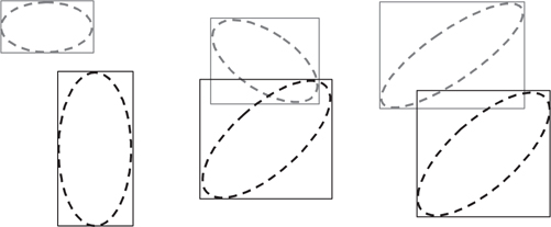
FIGURE 4.8
The intersection of error boxes offers a preliminary indication that a track and a report probably correspond to the same object. A more definitive test of correlation requires a computation to determine the extent to which the error ellipses (or their higher-dimensional analogs) overlap, but such computations can be too time-consuming when applied to many thousands of track-report pairs. Comparing bounding boxes is more computationally efficient; if they do not intersect, an assumption can be made that the track and report do not correspond to the same object. However, intersection does not necessarily imply that they do correspond to the same object. False positives must be weeded out in subsequent processing.

FIGURE 4.9
Structure of a ternary tree. In a ternary tree, the boxes in the left subtree fall on one side of the partitioning (split) plane, the boxes in the right subtree fall to the other side of the plane, and the boxes in the middle subtree are strictly cut by the plane.
The middle subtree represents obligatory search effort; therefore, one goal is to minimize the number of boxes that straddle the split value. However, if most of the nodes fall to the left or right of the split value, then few nodes will be eliminated from the search, and query performance will be degraded. Thus, a trade-off must be made between the effects of unbalance and of large middle subtrees. Techniques have been developed for adapting ternary trees to exploit distribution features of a given set of boxes,16 but they cannot easily be applied when boxes are inserted and deleted dynamically. The ability to dynamically update the search structure can be very important in some applications; this topic is addressed in subsequent sections of this chapter.
4.3 Priority kd-Trees
The ternary tree represents a very intuitive approach to extending the kd-tree for the storage of boxes. The idea is that, in one dimension, if a balanced tree is constructed from the minimum values of each interval, then the only problematic cases are those intervals whose min endpoints are less than a split value while their max endpoints are greater. Thus, if these cases can be handled separately (i.e., in separate subtrees), then the rest of the tree can be searched the same way as an ordinary binary search tree. This approach fails because it is not possible to ensure simultaneously that all subtrees are balanced and that the extra subtrees are sufficiently small. As a result, an entirely different strategy is required to bound the worst-case performance.
The priority search tree technique is known for extending binary search to the problem of finding intersections among one-dimensional intervals.18,19 This tree is constructed by sorting the intervals according to the first coordinate as in an ordinary one-dimensional binary search tree. Then down every possible search path, the intervals are ordered by the second endpoint. Thus, the intervals encountered by always searching the left subarray will all have values for their first endpoint that are less than those of intervals with larger indices (i.e., to their right). At the same time, though, the second endpoints in the sequence of intervals will be in ascending order. Because any interval whose second endpoint is less than the first endpoint of the query interval cannot possibly produce an intersection, an additional stopping criterion is added to the ordinary binary search algorithm.
The priority search tree avoids the problems associated with middle subtrees in a ternary tree by storing the min endpoints in an ordinary balanced binary search tree, while storing the max endpoints in priority queues stored along each path in the tree. This combination of data structures permits the storage of n intervals, such that intersection queries can be satisfied in worst-case O(log n + m) time, and insertions and deletions of intervals can be performed in worst-case O(log n) time. Thus, the priority search tree generalizes binary search on points to the case of intervals, without any penalty in terms of errors. Unfortunately, the priority search tree is defined purely for intervals in one dimension.
The kd-tree can store multidimensional points, but not multidimensional ranges, whereas the priority search tree can store one-dimensional ranges, but not multiple dimensions. The question that arises is whether the kd-tree can be extended to store boxes efficiently, or whether the priority search tree can be extended to accommodate the analog of intervals in higher dimensions (i.e., boxes). The answer to the question is “yes” for both data structures, and the solution is, in fact, a combination of the two.
A priority kd-tree20 is defined as follows: Given a set S of k-dimensional box intervals (loi, hii), 1 < i < k, a priority kd-tree consists of a kd-tree constructed from the lo endpoints of the intervals with a priority set containing up to k items stored at each node (Figure 4.10).*

FIGURE 4.10
Structure of a priority kd-tree. The priority kd-tree stores multidimensional boxes, instead of vectors. A box is defined by an interval (loi, hii) for each coordinate i. The partitioning is applied to the lo coordinates analogously to an ordinary kd-tree. The principal difference is that the maximum hi value for each coordinate is stored at each node. These hi values function analogously to the priority fields of a priority search tree. In searching a priority kd-tree, the query box is compared to each of the stored values at each visited node. If the node partitions on coordinate i, then the search proceeds to the left subtree if loi is less than the median loi associated with the node. If hii is greater than the median loi, then the right subtree must be searched. The search can be terminated, however, if for any j, loj of the query box is greater than the hij stored at the node.
The items stored at each node are the minimum set so that the union of the hi endpoints in each coordinate includes a value greater than the corresponding hi endpoint of any interval of any item in the subtree. Searching the tree proceeds exactly as for all ordinary priority search trees, except that the intervals compared at each level in the tree cycle through the k dimensions as in a search of a kd-tree.
The priority kd-tree can be used to efficiently satisfy box intersection queries. Just as important, however, is the fact that it can be adapted to accommodate the dynamic insertion and deletion of boxes in optimal O(log n) time by replacing the kd-tree structure with a divided kd-tree structure.21 The difference between the divided kd-tree and an ordinary kd-tree is that the divided variant constructs a d-layered tree in which each layer partitions the data structure according to only one of the d coordinates. In three dimensions, for example, the first layer would partition on the x coordinate, the next layer on y, and the last layer on z. The number of levels per layer/coordinate is determined so as to minimize query time complexity. The reason for stratifying the tree into layers for the different coordinates is to allow updates within the different layers to be treated just like updates in ordinary one-dimensional binary trees.
Associating priority fields with the different layers results in a dynamic variant of the priority kd-tree, which is referred to as a layered box tree. Note that the i priority fields, for coordinates l, …, i, need to be maintained at level i. This data structure has been proven17 to be maintainable at a cost of O(log n) time per insertion or deletion and can satisfy box intersection queries O(n1–1/k log1/k n + m), where m is the number of boxes in S that intersect a given query box. Application of an improved variant22 of the divided kd-tree improves the query complexity to O(n1–1/k + m), which is optimal.
The priority kd-tree is optimal among the class of linear-sized data structures, that is, those using only O(n) storage, but asymptotically better O(logk n + m) query complexity is possible if O(n logk–1 n) storage is used.12,13 However, the extremely complex structure, called a range-segment tree, requires O(logk n) update time, and the query performance is O(logk n + m). Unfortunately, this query complexity holds in the average case, as well as in the worst case, so it can be expected to provide superior query performance in practice only when n is extremely large. For realistic distributions of objects, however, it may never provide better query performance practice. Whether or not that is the case, the range-segment tree is almost never used in practice because the values of n1–1/k and logk n are comparable even for n as large as 1,000,000, and for data sets of that size, the storage for the range-segment tree is multiplied by a factor of log2(1,000,000) = 400.
Another data structure, called the DE-tree,23 has recently been described in the literature. It has suboptimal worst-case theoretical performance but practical performance that seems to exceed all other known data structures in a wide variety of experimental contexts. The DE-tree is of particular interest in target tracking because it can efficiently identify intersections between boxes and rays, which is necessary when tracking with bearings-only (i.e., line-of-sight) sensors.
4.3.1 Applying the Results
The method in which multidimensional search structures are applied in a tracking algorithm can be summarized as follows: tracks are recorded by storing the information—such as current positions, velocities, and accelerations—that a Kalman filter needs to estimate the future position of each candidate target. When a new batch of position reports arrives, the existing tracks are projected forward to the time of the reports. An error ellipsoid is calculated for each track and each report, and a box is constructed around each ellipsoid. The boxes representing the track projections are organized into a multidimensional tree. Each box representing a report becomes the subject of a complete tree search; the result of the search is the set of all track boxes that intersect the given report box. Track–report pairs whose boxes do not intersect are excluded from all further consideration. Next the set of track–report pairs whose boxes do overlap is examined more closely to see whether the inscribed error ellipsoids also overlap. Whenever this calculation indicates a correlation, the track is projected to the time of the new report. Tracks that consistently fail to be associated with any report are eventually deleted; reports that cannot be associated with any existing track initiate new tracks.
The above-mentioned approach for multiple-target tracking ignores a plethora of intricate theoretical and practical details. Unfortunately, such details must eventually be addressed, and the SDI forced a generation of tracking, data fusion, and sensor system researchers to face all of the thorny issues and constraints of a real-world problem of immense scale. The goal was to develop a space-based system to defend against a full-scale missile attack against the United States. Two of the most critical problems were the design and deployment of sensors to detect the launch of missiles at the earliest possible moment in their 20 min midcourse flight, and the design and deployment of weapons systems capable of destroying the detected missiles. Although an automatic tracking facility would clearly be an integral component of any SDI system, it was not generally considered a “high-risk” technology. Tracking, especially of aircraft, had been widely studied for more than 30 years, so the tracking of nonmaneuvering ballistic missiles seemed to be a relatively simple engineering exercise. The principal constraint imposed by SDI was that the tracking be precise enough to predict a missile’s future position to within a few meters, so that it could be destroyed by a high-energy laser or a particle-beam weapon.
The high-precision tracking requirement led to the development of highly detailed models of ballistic motion that took into account the effects of atmospheric drag and various gravitational perturbations over the earth. By far the most significant source of error in the tracking process, however, resulted from the limited resolution of existing sensors. This fact reinforced the widely held belief that the main obstacle to effective tracking was the relatively poor quality of sensor reports. The impact of large numbers of targets seemed manageable, just build larger, faster computers. Although many in the research community thought otherwise, the prevailing attitude among funding agencies was that if 100 objects could be tracked in real time, then little difficulty would be involved in building a machine that would be 100 times faster—or simply having 100 machines run in parallel—to handle 10,000 objects.
Among the challenges facing the SDI program, multiple-target tracking seemed far simpler than what would be required to further improve sensor resolution. This belief led to the awarding of contracts to build tracking systems in which the emphasis was placed on high precision at any cost in terms of computational efficiency. These systems did prove valuable for determining bounds on how accurately a single cluster of three to seven missiles could be tracked in an SDI environment, but ultimately pressures mounted to scale up to more realistic numbers. In one case, a tracker that had been tested on five missiles was scaled up to track 100, causing the processing time to increase from a couple of hours to almost a month of nonstop computation for a simulated 20 min scenario. The bulk of the computations were later determined to have involved the correlation step, where reports were compared against hypothesis tracks.
In response to a heightened interest in scaling issues, some researchers began to develop and study prototype systems based on efficient search structures. One of these systems demonstrated that 65–100 missiles could be tracked in real time on a late-1980s personal workstation. These results were based on the assumption that a good-resolution radar report would be received every 5 s for every missile, which is unrealistic in the context of SDI; nevertheless, the demonstration did provide convincing evidence that SDI trackers could be adapted to avoid quadratic scaling. A tracker that had been installed at the SDI National Testbed in Colorado Springs achieved significant performance improvements after a tree-based search structure was installed in its correlation routine; the new algorithm was superior for as few as 40 missiles. Stand-alone tests showed that the search component could process 5,000–10,000 range queries in real time on a modest computer workstation of the time. These results suggested that the problem of correlating vast numbers of tracks and reports had been solved. Unfortunately, a new difficulty was soon discovered.
The academic formulation of the problem adopts the simplifying assumption that all position reports arrive in batches, with all the reports in a batch corresponding to measurements taken at the same instant of all of the targets. A real distributed sensor system would not work this way; reports would arrive in a continuing stream and would be distributed over time. To determine the probability that a given track and report correspond to the same object, the track must be projected to the measurement time of the report. If every track has to be projected to the measurement time of every report, the combinatorial advantages of the tree-search algorithm are lost.
A simple way to avoid the projection of each track to the time of every report is to increase the search radius in the gating algorithm to account for the maximum distance an object could travel during the maximum time difference between any track and report. For example, if the maximum speed of a missile is 10 km/s, and the maximum time difference between any report and track is 5 s, then 50 km would have to be added to each search radius to ensure that no correlations are missed. For boxes used to approximate ellipsoids, this means that each side of the box must be increased by 100 km.
As estimates of what constitutes a realistic SDI scenario became more accurate, members of the tracking community learned that successive reports of a particular target often would be separated by as much as 30–40 s. To account for such large time differences would require boxes so immense that the number of spurious returns would negate the benefits of efficient search. Demands for a sensor configuration that would report on every target at intervals of 5–10 s were considered unreasonable for a variety of practical reasons. The use of sophisticated correlation algorithms seemed to have finally reached its limit. Several heuristic “fixes” were considered, but none solved the problem.
A detailed scaling analysis of the problem ultimately pointed the way to a solution. Simply accumulate sensor reports until the difference between the measurement time of the current report and the earliest report exceeds a threshold. A search structure is then constructed from this set of reports, the tracks are projected to the mean time of the reports, and the correlation process is performed with the maximum time difference being no more than half of the chosen time-difference threshold. The subtle aspect of this deceptively simple approach is the selection of the threshold. If it is too small, every track will be projected to the measurement time of every report. If it is too large, every report will fall within the search volume of every track. A formula has been derived that, with only modest assumptions about the distribution of targets, ensures the optimal trade-off between these two extremes.
Although empirical results confirm that the track file projection approach essentially solves the time difference problem in most practical applications, significant improvements are possible. For example, the fact that different tracks are updated at different times suggests that projecting all of the tracks at the same points in time may be wasteful. An alternative approach might take a track updated with a report at time ti and construct a search volume sufficiently large to guarantee that the track gates with any report of the target arriving during the subsequent s seconds, where s is a parameter similar to the threshold used for triggering track file projections. This is accomplished by determining the region of space the target could conceivably traverse based on its kinematic state and error covariance. The box circumscribing this search volume can then be maintained in the search structure until time ti + s, at which point it becomes stale and must be replaced with a search volume that is valid from time ti + s to time ti + 2s. However, if before becoming stale it is updated with a report at time tj, ti < tj < ti + s, then it must be replaced with a search volume that is valid from time tj to time tj + s.
The benefit of the enhanced approach is that each track is projected only at the times when it is updated or when all extended period has passed without an update (which could possibly signal the need to delete the track). To apply the approach, however, two conditions must be satisfied. First, there must be a mechanism for identifying when a track volume has become stale and needs to be recomputed. It is, of course, not possible to examine every track upon the receipt of each report because the scaling of the algorithm would be undermined. The solution is to maintain a priority queue of the times at which the different track volumes will become invalid. A priority queue is a data structure that can be updated efficiently and supports the retrieval of the minimum of n values in O(log n) time. At the time a report is received, the priority queue is queried to determine which, if any, of the track volumes have become stale. New search volumes are constructed for the identified tracks, and the times at which they will become invalid are updated in the priority queue.
The second condition that must be satisfied for the enhanced approach is a capability to incrementally update the search structure as tracks are added, updated, recomputed, or deleted. The need for such a capability was hinted at in the discussion of dynamic search structures. Because the layered box tree supports insertions and deletions in O(log n) time, the update of a track’s search volume can be efficiently accommodated. The track’s associated box is deleted from the tree, an updated box is computed, and then the result is inserted back into the tree. In summary, the cost for processing each report involves updates of the search structure and the priority queue, at O(log n) cost, plus the cost of determining the set of tracks with which the report could be feasibly associated.
4.4 Conclusion
The correlation of reports with tracks numbering in thousands can now be performed in real time on a personal computer. More research on large-scale correlation is needed, but work has already begun on implementing efficient correlation modules that can be incorporated into existing tracking systems. Ironically, by hiding the intricate details and complexities of the correlation process, these modules give the appearance that multiple-target tracking involves little more than the concurrent processing of several single-target problems. Thus, a paradigm with deep historical roots in the field of target tracking is at least partially preserved.
Note that the techniques described in this chapter are applicable only to a very restricted class of tracking problems. Other problems, such as the tracking of military forces, demand more sophisticated approaches. Not only does the mean position of a military force change, its shape also changes. Moreover, reports of its position are really only reports of the positions of its parts, and various parts may be moving in different directions at any given instant. Filtering out the local deviations in motion to determine the net motion of the whole is beyond the capabilities of a simple Kalman filter. Other difficult tracking problems include the tracking of weather phenomena and soil erosion. The history of multiple-target tracking suggests that, in addition to new mathematical techniques, new algorithmic techniques will certainly be required for any practical solution to these problems.
Acknowledgment
The author gratefully acknowledges support from the Naval Research Laboratory, Washington, DC.
References
1. Uhlmann, J.K., Algorithms for multiple-target tracking, American Scientist, 80(2): 128–141, 1992.
2. Kalman, R.E., A new approach to linear filtering and prediction problems, ASME, Basic Engineering, 82: 34–45, 1960.
3. Blackman, S.S., Multiple-Target Tracking with Radar Applications, Artech House, Norwood, MA, 1986.
4. Bar Shalom, Y. and Fortmann, T.E., Tracking and Data Association, Academic Press, New York, NY, 1988.
5. Blackman, S. and Popoli R., Design and Analysis of Modern Tracking Systems, Artech House, Norwood, MA, 1999.
6. Bar Shalom, Y. and Li, X.R., Multitarget-Multisensor Tracking: Principles and Techniques, YBS Press, New York, NY, 1995.
7. Uhlmann, J.K., Zuniga, M.R., and Picone, J.M., Efficient approaches for report/cluster correlation in multi-target tracking systems, NRL Report 9281, US Government, Washington, DC, 1990.
8. Bentley, J., Multidimensional binary search trees for associative searching, Communications of the ACM, 18(9): 509–517, 1975.
9. Yianilos, P.N., Data structures and algorithms for nearest neighbor search in general metric spaces, in SODA, Austin, TX, pp. 311–321, 1993.
10. Uhlmann, J.K., Implementing metric trees to satisfy general proximity/similarity queries, NRL Code 5570 Technical Report 9192, 1992.
11. Lee, D.T. and Wong, C.K., Worse-case analysis for region and partial region searches in multidimensional binary search trees and quad trees, Acta Informatica, 9(1): 23–29, 1977.
12. Preparata, F. and Shamos, M., Computational Geometry, Springer-Verlag, New York, NY, 1985.
13. Mehlhorn, K., Multidimensional Searching and Computational Geometry, Vol. 3, Springer-Verlag, Berlin, 1984.
14. Uhlmann, J.K. and Zuniga, M.R., Results of an efficient gating algorithm for large-scale tracking scenarios, Naval Research Reviews, 43(1): 24–29, 1991.
15. Zuniga, M.R., Picone, J.M., and Uhlmann, J.K., Efficient algorithm for unproved gating combinatorics in multiple-target tracking, submitted to IEEE Transactions on Aerospace and Electronic Systems, 1990.
16. Uhlmann, J.K., Adaptive partitioning strategies for ternary tree structures, Pattern Recognition Letters, 12(9): 537–541, 1991.
17. Boroujerdi, A. and Uhlmann, J.K., Large-scale intersection detection using layered box trees, AIT-DSS Report, US Government, 1998.
18. McCreight, E.M., Priority search trees, SIAM Journal of Computing, 14(2): 257–276, 1985.
19. Wood, D., Data, Structures, Algorithms, and Performance, Addison-Wesley Longman, Boston, MA, 1993.
20. Uhlmann, J.K., Dynamic map building and localization for autonomous vehicles, Engineering Sciences Report, Oxford University, London, UK, 1994.
21. van Kreveld, M. and Overmars, M., Divided k-d trees, Algorithmica, 6: 840–858, 1991.
22. Kanth, K.V.R. and Singh, A., Optimal dynamic range searching in non-replicating index structures, in Lecture Notes in Computer Science, Vol. 1540, pp. 257–276, Springer, Berlin, 1999.
23. Zuniga, M.R. and Uhlmann, J.K., Ray queries with wide object isolation with DE-trees, Journal of Graphics Tools, 11(3): 19–37, 2006.
24. Ramasubramanian, V. and Paliwal, K., An efficient approximation-elimination algorithm for fast nearest-neighbour search on a spherical distance coordinate formulation, Pattern Recognition Letters, 13(7): 471–480, 1992.
25. Vidal, E., An algorithm for finding nearest neighbours in (approximately) constant average time complexity, Pattern Recognition Letters, 4(3): 145–157, 1986.
26. Vidal, E., Rulot, H., Casacuberta, F., and Benedi, J.M., On the use of a metric-space search algorithm (AESA) for fast DTW-based recognition of isolated words, IEEE Transactions on Acoustics, Speech, and Signal Processing, 36(5): 651–660, 1988.
27. Uhlmann, J.K., Metric trees, Applied Mathematics Letters, 4(5): 61–62, 1991.
28. Uhlmann, J.K., Satisfying general proximity/similarity queries with metric trees, Information Processing Letters, 40: 175–170, 1991.
29. Collins, J.B. and Uhlmann, J.K., Efficient gating in data association for multivariate Gaussian distributions, IEEE Transactions on Aerospace and Electronic Systems, 28(3): 909–916, 1990.
* The material in this chapter updates and supplements material that first appeared in American Scientist.1
* An alternative generalization of binary search to multiple dimensions is to partition the data set at each stage according to its distance from a selected set of points:9,10,24, 25, 26, 27 and 28 those that are less than the median distance comprise one branch of the tree, and those that are greater comprise the other. These data structures are very flexible because they offer the freedom to use an appropriate application-specific metric to partition the data set; however, they are also much more computationally intensive because of the number of distance calculations that must be performed.
* Other data structures have been independently called priority kd-trees in the literature, but they are different data structures designed for different purposes.