14 General Decentralized Data Fusion with Covariance Intersection

Decentralized (or distributed) data fusion (DDF) is one of the most important areas of research in the field of control and estimation. The motivation for decentralization is that it provides a degree of scalability and robustness that cannot be achieved using traditional centralized architectures. In industrial applications, decentralization offers the possibility of producing plug-and-play systems in which sensors of different types and capabilities can be slotted in and out, optimizing trade-offs such as price, power consumption, and performance. This has significant implications for military systems as well because it can dramatically reduce the time required to incorporate new computational and sensing components into fighter aircraft, ships, and other types of platforms.

The benefits of decentralization are not limited to sensor fusion aboard a single platform; decentralization makes it possible for a network of platforms to exchange information and coordinate activities in a flexible and scalable fashion. Interplatform information propagation and fusion form the crux of the network centric warfare (NCW) vision for the U.S. military. The goal of NCW is to equip all battlespace entities—aircraft, ships, and even individual human combatants—with communication and computing capabilities such that each becomes a node in a vast decentralized command and control network. The idea is that each entity can dynamically establish a communication link with any other entity to obtain the information it needs to perform its warfighting role.

Although the notion of decentralization has had strong intuitive appeal for several decades, achieving its anticipated benefits has proven extremely difficult. Specifically, implementers quickly discovered that if communication paths are not strictly controlled, pieces of information begin to propagate redundantly. When these pieces of information are reused (i.e., double-counted), the fused estimates produced at different nodes in the network become corrupted. Various approaches for avoiding this problem were examined, but none seemed completely satisfactory. In the mid-1990s, the redundant information problem was revealed to be far more than just a practical challenge; it is a manifestation of a fundamental theoretical limitation that could not be surmounted using traditional Bayesian control and estimation methods such as the Kalman filter.¹ In response to this situation, a new data fusion framework, based on covariance intersection (CI), was developed. The CI framework effectively supports all aspects of general DDF.

The structure of this chapter is as follows: Section 14.2 describes the DDF problem. The CI algorithm is described in Section 14.3. Section 14.4 demonstrates how CI supports DDF and describes one such distribution architecture. A simple example of a network with redundant links is presented in Section 14.5. Section 14.6 shows how to exploit known information about network connectivity and information proliferation within the CI framework. Section 14.7 describes recent proposed generalizations of CI to explicit probability distributions, and describes a tractable approximation for Gaussian mixture models. This chapter concludes with a brief discussion on other applications of CI.

14.2 Decentralized Data Fusion

A DDF system is a collection of processing nodes, connected by communication links (Figure 14.1), in which none of the nodes has knowledge about the overall network topology. Each node performs a specific computing task using information from nodes with which it is linked, but no central node exists that controls the network. There are many attractive properties of such decentralized systems,² including

Decentralized systems are reliable in the sense that the loss of a subset of nodes and links does not necessarily prevent the rest of the system from functioning. In a centralized system, however, the failure of a common communication manager or a centralized controller can result in immediate catastrophic failure of the system.
Decentralized systems are flexible in the sense that nodes can be added or deleted by making only local changes to the network. For example, the addition of a node simply involves the establishment of links to one or more nodes in the network. In a centralized system, however, the addition of a new node can change the topology in such a way that the overall control and communications structure require massive changes.

The most important class of decentralized networks involves nodes associated with sensors or other information sources (such as databases of a priori information). Information from distributed sources propagates through the network so that each node obtains the data relevant to its own processing task. In a battle management application, for example, one node might be associated with the acquisition of information from reconnaissance photographs, another with ground-based reports of troop movements, and another with the monitoring of communication transmissions. Information from these nodes could then be transmitted to a node that estimates the position and movement of enemy troops. The information from this node could then be transmitted back to the reconnaissance photo node, which would use the estimated positions of troops to aid in the interpretation of ambiguous features in satellite photos.

Images

FIGURE 14.1
A distributed data fusion network. Each box represents a fusion node. Each node possesses 0 or more sensors and is connected to its neighboring nodes through a set of communication links.

In most applications, the information propagated through a network is converted into a form that provides the estimated state of some quantity of interest. In many cases, especially in industrial applications, the information is converted into means and covariances that can be combined within the framework of Kalman-type filters. A decentralized network for estimating the position of a vehicle, for example, could combine acceleration estimates from nodes measuring wheel speed, from laser gyros, and from pressure sensors on the accelerator pedal. If each independent node provides the mean and variance of its estimate of acceleration, fusing the estimates to obtain a better-filtered estimate is relatively easy.

The most serious problem arising in DDF networks is the effect of redundant information.³ Specifically, pieces of information from multiple source cannot be combined within most filtering frameworks unless they are independent or have a known degree of correlation (i.e., known cross covariances). In the battle management example described in the preceding text, the effect of redundant information can be seen in the following scenario, sometimes referred to as rumor propagation or the whispering in the hall problem:

A photoreconnaissance node transmits information about potentially important features. This information then propagates through the network, changing form as it is combined with information at other nodes in the process.
The troop position estimation node eventually receives the information in some form and notes that one of the indicated features could possibly represent a mobilizing tank battalion at position x. There are many other possible interpretations of the feature, but the possibility of a mobilizing tank battalion is deemed to be of such tactical importance that it warrants the transmission of a low confidence hypothesis (a heads up message). Again, the information can be synopsized, augmented, or otherwise transformed as it is relayed through a sequence of nodes.
The photoreconnaissance photo node receives the low confidence hypothesis that a tank battalion may have mobilized at position x. A check of available reconnaissance photos covering position x reveals a feature that is consistent with the hypothesis. Because the node is unaware that the hypothesis was based on that same photographic evidence, it assumes that the feature that it observes is an independent confirmation of the hypothesis. The node then transmits high confidence information that a feature at position x represents a mobilizing tank battalion.
The troop position node receives information from the photoreconnaissance node that a mobilizing tank battalion has been identified with high confidence. The troop position node regards this as confirmation of its early hypothesis and calls for an aggressive response to the mobilization.

The obvious problem is that the two nodes exchange redundant pieces of information and treat them as independent pieces of evidence in support of the hypothesis that a tank battalion has mobilized. The end result is that critical resources may be diverted in reaction to what is, in fact, a low probability hypothesis.

A similar situation can arise in a decentralized monitoring system for a chemical process:

A reaction vessel is fitted with a variety of sensors, including a pressure gauge.
Because the bulk temperature of the reaction cannot be measured directly, a node is added that uses pressure information, combined with a model of the reaction, to estimate temperature.
A new node is added to the system that uses information from the pressure and temperature nodes.

Clearly, the added node will always use redundant information from the pressure gauge. If the estimates of pressure and temperature are treated as independent, then the fact that their relationship is always exactly what is predicted by the model might lead to overconfidence in the stability of the system. This type of inadvertent use of redundant information arises commonly when attempts are made to decompose systems into functional modules. The following example is typical:

A vehicle navigation and control system maintains one Kalman filter for estimating position and a separate Kalman filter for maintaining the orientation of the vehicle.
Each filter uses the same sensor information.
The full vehicle state is determined (for prediction purposes) by combining the position and orientation estimates.
The predicted position covariance is computed essentially as a sum of the position and orientation covariances (after the estimates are transformed to a common vehicle coordinate frame).

The problem in this example is that the position and orientation errors are not independent. This means that the predicted position covariance will underestimate the actual position error. Obviously, such overly confident position estimates can lead to unsafe maneuvers.

To avoid the potentially disastrous consequences of redundant data on Kalman-type estimators, covariance information must be maintained. Unfortunately, maintaining consistent cross covariances in arbitrary decentralized networks is not possible locally.¹ In only a few special cases, such as tree and fully connected networks, can the proliferation of redundant information be avoided. These special topologies, however, fail to provide the reliability advantage because the failure of a single node or link results in either a disconnected network or one that is no longer able to avoid the effects of redundant information. Intuitively, the redundancy of information in a network is what provides reliability; therefore, if the difficulties with redundant information are avoided by eliminating redundancy, then reliability will also be eliminated.

The proof that cross covariance information cannot be consistently maintained in general decentralized networks seems to imply that the supposed benefits of decentralization are unattainable. However, the proof relies critically on the assumption that some knowledge of the degree of correlation is necessary to fuse pieces of information. This is certainly the case for all classical data fusion mechanisms (e.g., the Kalman filter and Bayesian nets), which are based on applications of Bayes’ rule. Furthermore, independence assumptions are also implicit in many ad hoc schemes that compute averages over quantities with intrinsically correlated error components.*

The problems associated with assumed independence are often side stepped by artificially increasing the covariance of the combined estimate. This heuristic (or filter tuning) can prevent the filtering process from producing nonconservative estimates, but substantial empirical analysis and tweaking is required to determine the extent of increase in the covariances. Even with this empirical analysis, the integrity of the Kalman filter framework is compromised, and reliable results cannot be guaranteed. In many applications, such as in large decentralized signal/data fusion networks, the problem is much more acute and no amount of heuristic tweaking can avoid the limitations of the Kalman filter framework.² This is of enormous consequence, considering the general trend toward decentralization in complex military and industrial systems.

In summary, the only plausible way to simultaneously achieve robustness and consistency in a general decentralized network is to exploit a data fusion mechanism that does not require independence assumptions. Such a mechanism called CI satisfies this requirement.

14.3 Covariance Intersection

14.3.1 Problem Statement

Consider the following problem. Two pieces of information, labeled A and B, are to be fused together to yield an output, C. This is a very general type of data fusion problem. A and B could be two different sensor measurements (e.g., a batch estimation or track initialization problem), or A could be a prediction from a system model and B could be sensor information (e.g., a recursive estimator similar to a Kalman filter). Both terms are corrupted by measurement noises and modeling errors; therefore, their values are known imprecisely and A and B are the random variables a and b, respectively. Assume that the true statistics of these variables are unknown. The only available information are estimates of the means and covariances of a and b and the cross correlations between them, which are {a, P_aa}, {b, P_bb}, and 0, respectively.*

\begin{matrix} {\bar{P}}_{aa} = E [\tilde{a} {\tilde{a}}^{T}], {\bar{P}}_{ab} = E [\tilde{a} {\tilde{b}}^{T}], {\bar{P}}_{bb} = E [\tilde{b} {\tilde{b}}^{T}] & (14.1) \end{matrix}

$\begin{matrix} {\bar{P}}_{aa} = E [\tilde{a} {\tilde{a}}^{T}], {\bar{P}}_{ab} = E [\tilde{a} {\tilde{b}}^{T}], {\bar{P}}_{bb} = E [\tilde{b} {\tilde{b}}^{T}] & (14.1) \end{matrix}$

where $\tilde{a} \equiv a - \bar{a}$ $\tilde{a} \equiv a - \bar{a}$ and $\tilde{b} \equiv b - \bar{b}$ $\tilde{b} \equiv b - \bar{b}$ are the true errors imposed by assuming that the means are a and b. Note that the cross correlation matrix between the random variables, ${\bar{P}}_{ab}$ ${\bar{P}}_{ab}$ , is unknown and will not, in general, be 0.

The only constraint that we impose on the assumed estimate is consistency. In other words,

\begin{matrix} \begin{matrix} P_{aa} - {\bar{P}}_{aa} \geq 0 \\ P_{bb} - {\bar{P}}_{bb} \geq 0 \end{matrix} & (14.2) \end{matrix}

$\begin{matrix} \begin{matrix} P_{aa} - {\bar{P}}_{aa} \geq 0 \\ P_{bb} - {\bar{P}}_{bb} \geq 0 \end{matrix} & (14.2) \end{matrix}$

This definition conforms to the standard definition of consistency.⁴ The problem is to fuse the consistent estimates of A and B together to yield a new estimate C, {c, P_cc}, which is guaranteed to be consistent:

\begin{matrix} \begin{matrix} P_{cc} - {\bar{P}}_{cc} \geq 0 \end{matrix} & (14.3) \end{matrix}

$\begin{matrix} \begin{matrix} P_{cc} - {\bar{P}}_{cc} \geq 0 \end{matrix} & (14.3) \end{matrix}$

where $\tilde{c} \equiv c - \bar{c}$ $\tilde{c} \equiv c - \bar{c}$ and ${\bar{P}}_{cc} = E [\tilde{c} {\tilde{c}}^{T}]$ ${\bar{P}}_{cc} = E [\tilde{c} {\tilde{c}}^{T}]$ .

It is important to note that two estimates with different means do not, in general, supply additional information that can be used in the filtering algorithm.

14.3.2 Covariance Intersection Algorithm

In its generic form, the CI algorithm takes a convex combination of mean and covariance estimates expressed in information (or inverse covariance) space. The intuition behind this approach arises from a geometric interpretation of the Kalman filter equations. The general form of the Kalman filter equation can be written as

\begin{matrix} \bar{c} = W_{a} \bar{a} + W_{a} \bar{b} & (14.4) \end{matrix}

$\begin{matrix} \bar{c} = W_{a} \bar{a} + W_{a} \bar{b} & (14.4) \end{matrix}$

\begin{matrix} P_{cc} = W_{a} P_{aa} W_{a}^{T} + W_{a} P_{ab} W_{b}^{T} + W_{b} P_{ba} W_{a}^{T} + W_{b} P_{bb} W_{b}^{T} & (14.5) \end{matrix}

$\begin{matrix} P_{cc} = W_{a} P_{aa} W_{a}^{T} + W_{a} P_{ab} W_{b}^{T} + W_{b} P_{ba} W_{a}^{T} + W_{b} P_{bb} W_{b}^{T} & (14.5) \end{matrix}$

where the weights W_a and W_b are chosen to minimize the trace of P_cc. This form reduces to the conventional Kalman filter if the estimates are independent (P_ab = 0) and generalizes to the Kalman filter with colored noise when the correlations are known.

These equations have a powerful geometric interpretation: if one plots the covariance ellipses (for a covariance matrix P this is the locus of points {p : p^T P⁻¹ p = c} where c is a constant), P_aa, P_bb, and P_cc for all choices of P_ab, then P_cc always lies within the intersection of P_aa and P_bb. Figure 14.2 illustrates this for a number of different choices of P_ab.

Images

FIGURE 14.2
The shape of the updated covariance ellipse. The variances of P_aa and P_bb are the outer solid ellipses. Different values of P_cc that arise from different choices of P_ab are shown as dashed ellipses. The update with truly independent estimates is the inner solid ellipse.

This interpretation suggests the following approach: if P_cc lies within the intersection of P_aa and P_bb for any possible choice of P_ab, then an update strategy that finds a P_cc that encloses the intersection region must be consistent even if there is no knowledge about P_ab. The tighter the updated covariance encloses the intersection region, the more effectively the update uses the available information.*

The intersection is characterized by the convex combination of the covariances, and the CI algorithm is⁵

\begin{matrix} P_{cc}^{- 1} = ω P_{aa}^{- 1} + (1 - ω) P_{bb}^{- 1} & (14.6) \end{matrix}

$\begin{matrix} P_{cc}^{- 1} = ω P_{aa}^{- 1} + (1 - ω) P_{bb}^{- 1} & (14.6) \end{matrix}$

\begin{matrix} P_{cc}^{- 1} c = ω P_{aa}^{- 1} a + (1 - ω) P_{bb}^{- 1} b & (14.7) \end{matrix}

$\begin{matrix} P_{cc}^{- 1} c = ω P_{aa}^{- 1} a + (1 - ω) P_{bb}^{- 1} b & (14.7) \end{matrix}$

where ω ∈ [0, 1]. Appendix 14.A proves that this update equation is consistent in the sense given by Equation 14.3 for all choices of P_ab and ω.

As illustrated in Figure 14.3, the free parameter ω manipulates the weights assigned to a and b. Different choices of ω can be used to optimize the update with respect to different performance criteria, such as minimizing the trace or the determinant of P_cc. Cost functions, which are convex with respect to ω, have only one distinct optimum in the range 0 ≤ ω ≤ 1. Virtually any optimization strategy can be used, ranging from Newton-Raphson to sophisticated semidefinite and convex programming⁶ techniques, which can minimize almost any norm. Appendix 14.B includes source code for optimizing ω for the fusion of two estimates.

Note that some measure of covariance size must be minimized at each update to guarantee nondivergence; otherwise, an updated estimate could be larger than the prior estimate. For example, if one were always to use ω = 0.5, then the updated estimate would simply be the Kalman updated estimate with the covariance inflated by a factor of 2. Thus, an update with an observation that has a very large covariance could result in an updated covariance close to twice the size of the prior estimate. In summary, the use of a fixed measure of covariance size with the CI equations leads to the nondivergent CI filter.

Images

FIGURE 14.3
The value of ω determines the relative weights applied to each information term. (a) Shows the 1-sigma contours for 2D covariance matrices A and B and (b–d) show the updated covariance C (drawn in a solid line) for several different values of ω. For each value of ω, C passes through the intersection points of A and B.

An example of the tightness of the CI update can be seen in Figure 14.4 for the case when the two prior covariances approach singularity:

\begin{matrix} {a, A} = {[\begin{matrix} 1 \\ 0 \end{matrix}], [\begin{matrix} 1.5 & 0.0 \\ 0.0 & ɛ \end{matrix}]} & (14.8) \end{matrix}

$\begin{matrix} {a, A} = {[\begin{matrix} 1 \\ 0 \end{matrix}], [\begin{matrix} 1.5 & 0.0 \\ 0.0 & ɛ \end{matrix}]} & (14.8) \end{matrix}$

\begin{matrix} {b, B} = {[\begin{matrix} 0 \\ 1 \end{matrix}], [\begin{matrix} ɛ & 0.0 \\ 0.0 & 1.0 \end{matrix}]} & (14.9) \end{matrix}

$\begin{matrix} {b, B} = {[\begin{matrix} 0 \\ 1 \end{matrix}], [\begin{matrix} ɛ & 0.0 \\ 0.0 & 1.0 \end{matrix}]} & (14.9) \end{matrix}$

Images

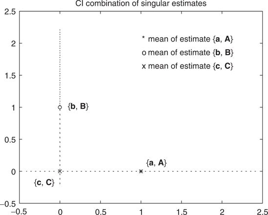
FIGURE 14.4
The CI update {c, C} of two 2D estimates {a, A} and {b, B}, where A and B are singular, defines the point of intersection of the colinear sigma contours of A and B.

The covariance of the combined estimate is proportional to ε, and the mean is centered on the intersection point of the 1D contours of the prior estimates. This makes sense intuitively because, if one estimate completely constrains one coordinate, and the other estimate completely constrains the other coordinate, there is only one possible update that can be consistent with both constraints.

CI can be generalized to an arbitrary number of n > 2 updates using the following equations:

\begin{matrix} P_{cc}^{- 1} = ω_{1} P_{a_{1} a_{1}}^{- 1} + ... + ω_{n} P_{a_{n} a_{n}}^{- 1} & (14.10) \end{matrix}

$\begin{matrix} P_{cc}^{- 1} = ω_{1} P_{a_{1} a_{1}}^{- 1} + ... + ω_{n} P_{a_{n} a_{n}}^{- 1} & (14.10) \end{matrix}$

\begin{matrix} P_{cc}^{- 1} c = ω_{1} P_{a_{1} a_{1}}^{- 1} a_{1} + ... + ω_{n} P_{a_{n} a_{n}}^{- 1} a_{n} & (14.11) \end{matrix}

$\begin{matrix} P_{cc}^{- 1} c = ω_{1} P_{a_{1} a_{1}}^{- 1} a_{1} + ... + ω_{n} P_{a_{n} a_{n}}^{- 1} a_{n} & (14.11) \end{matrix}$

where $Σ_{i = 1}^{n} ω_{i} = 1$ $Σ_{i = 1}^{n} ω_{i} = 1$ . For this type of batch combination of large numbers of estimates, efficient codes such as the public domain MAXDET⁷ and SPDSOL⁸ are available. Some generalizations for low-dimensional spaces have been derived.

In summary, CI provides a general update algorithm that is capable of yielding an updated estimate even when the prediction and observation correlations are unknown.

14.4 Using Covariance Intersection for Distributed Data Fusion

Consider again the data fusion network that is illustrated in Figure 14.1. The network consists of N nodes whose connection topology is completely arbitrary (i.e., it might include loops and cycles) and can change dynamically. Each node has information only about its local connection topology (e.g., the number of nodes with which it directly communicates and the type of data sent across each communication link). Assuming that the process and observation noises are independent, the only source of unmodeled correlations is the DDF system itself.

Images

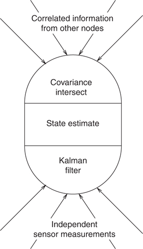
FIGURE 14.5
A canonical node in a general data fusion network that constructs its local state estimate using CI to combine information received from other nodes and a Kalman filter to incorporate independent sensor measurements.

CI can be used to develop a DDF algorithm that directly exploits this structure. The basic idea is illustrated in Figure 14.5. Estimates that are propagated from other nodes are correlated to an unknown degree and fused with the state estimate using CI. Measurements taken locally are known to be independent and can be fused using the Kalman filter equations.

Using conventional notation,⁹ the estimate at the ith node is ${\hat{x}}_{i} (k | k)$ ${\hat{x}}_{i} (k | k)$ with covariance P_i(k|k). CI can be used to fuse the information that is propagated between the different nodes. Suppose that, at time step k + 1, node i locally measures the observation vector z_i(k|k). A distributed fusion algorithm for propagating the estimate from time step k to time step k + 1 for node i is

Predict the state of node i at time k + 1 using the standard Kalman filter prediction equations.
Use the Kalman filter update equations to update the prediction with z_i(k + 1). This update is the distributed estimate with mean ${\hat{x}}_{i} (k + 1 | k + 1)$ ${\hat{x}}_{i} (k + 1 | k + 1)$ and covariance P_i(k + 1|k + 1). It is not the final estimate, because it does not include observations and estimates propagated from the other nodes in the network.
Node i propagates its distributed estimate to all of its neighbors.
Node i fuses its prediction ${\hat{x}}_{i} (k + 1 | k + 1)$ ${\hat{x}}_{i} (k + 1 | k + 1)$ and P_i(k + 1|k) with the distributed estimates that it has received from all of its neighbors to yield the partial update with mean ${\hat{x}}_{i}^{+} (k + 1 | k + 1)$ ${\hat{x}}_{i}^{+} (k + 1 | k + 1)$ and covariance $P_{i}^{+} (k + 1 | k + 1)$ $P_{i}^{+} (k + 1 | k + 1)$ . Because these estimates are propagated from other nodes whose correlations are unknown, the CI algorithm is used. As explained earlier, if the node receives multiple estimates for the same time step, the batch form of CI is most efficient. Finally, node i uses the Kalman filter update equations to fuse z_i(k + 1) with its partial update to yield the new estimate ${\hat{x}}_{i} (k + 1 | k + 1)$ ${\hat{x}}_{i} (k + 1 | k + 1)$ with covariance P_i(k + 1|k + 1). The Kalman filter equations are used because these are known to be independent of the prediction or data that has been distributed to the node from its neighbors. Therefore, CI is unnecessary. This concept is illustrated in Figure 14.5.

An implementation of this algorithm is given in Section 14.5. This algorithm has a number of important advantages. First, all nodes propagate their most accurate partial estimates to all other nodes without imposing any unrealistic requirements for perfectly robust communication. Communication paths may be uni- or bidirectional, there may be cycles in the network, and some estimates may be lost whereas others are propagated redundantly. Second, the update rates of the different filters do not need to be synchronized. Third, communications do not have to be guaranteed—a node can broadcast an estimate without relying on other nodes receiving it. Finally, each node can use a different observation model: one node may have a high accuracy model for one subset of variables of relevance to it, and another node may have a high accuracy model for a different subset of variables, but the propagation of their respective estimates allows nodes to construct fused estimates representing the union of the high accuracy information from both nodes.

The most important feature of this approach to DDF is that it is provably guaranteed to produce and maintain consistent estimates at the various nodes.* Section 14.5 demonstrates this consistency in a simple example.

14.5 Extended Example

Suppose the processing network, shown in Figure 14.6, is used to track the position, velocity, and acceleration of a 1D particle. The network is composed of four nodes. Node 1 measures the position of the particle only. Nodes 2 and 4 measure velocity and node 3 measures acceleration. The four nodes are arranged in a ring. From a practical standpoint, this configuration leads to a robust system with built-in redundancy: data can flow from one node to another through two different pathways. However, from a theoretical point of view, this configuration is extremely challenging. Because this configuration is neither fully connected nor tree connected, optimal data fusion algorithms exist only in the special case where the network topology and the states at each node are known.

Images

FIGURE 14.6
The network layout for our extended example.

TABLE 14.1
Sensor Information and Accuracy for Each Node from Figure 14.6

Node	Measures	Variances
1	x	1
2	$\dot{x}$ $\dot{x}$	2
3	$\ddot{x}$ $\ddot{x}$	0.25
4	$\dot{x}$ $\dot{x}$	3

The particle moves using a nominal constant acceleration model with process noise injected into the jerk (derivative of acceleration). Assuming that the noise is sampled at the start of the time step and is held constant throughout the prediction step, the process model is

\begin{matrix} X_{(k + 1)} = F x_{(k)} + G v_{(k + 1)} & (14.12) \end{matrix}

$\begin{matrix} X_{(k + 1)} = F x_{(k)} + G v_{(k + 1)} & (14.12) \end{matrix}$

where

\begin{matrix} F = [\begin{matrix} 1 & Δ T & Δ T^{2} / 2 \\ 0 & 1 & Δ T \\ 0 & 0 & 1 \end{matrix}] & and & G = [\begin{matrix} Δ T^{3} / 6 \\ Δ T^{2} / 2 \\ Δ T \end{matrix}] \end{matrix}

$\begin{matrix} F = [\begin{matrix} 1 & Δ T & Δ T^{2} / 2 \\ 0 & 1 & Δ T \\ 0 & 0 & 1 \end{matrix}] & and & G = [\begin{matrix} Δ T^{3} / 6 \\ Δ T^{2} / 2 \\ Δ T \end{matrix}] \end{matrix}$

ν(k) is an uncorrelated, zero-mean Gaussian noise with variance σ^2ν = 10 and length of the time step ∆T = 0.1 s.

The sensor information and the accuracy of each sensor are given in Table 14.1.

Assume, for the sake of simplicity, that the structure of the state space and the process models are the same for each node and are the same as the true system. However, this condition is not particularly restrictive and many of the techniques of model and system distribution that are used in optimal data distribution networks can be applied with CI.¹⁰

The state at each node is predicted using the process model:

\begin{matrix} \hat{x} (k + 1 | k) & = F {\hat{x}}_{i} (k | k) \\ P_{i} (k + 1 | k) & = {FP}_{i} (k + 1 | k) F^{T} + Q (k) \end{matrix}

$\begin{matrix} \hat{x} (k + 1 | k) & = F {\hat{x}}_{i} (k | k) \\ P_{i} (k + 1 | k) & = {FP}_{i} (k + 1 | k) F^{T} + Q (k) \end{matrix}$

The partial estimates ${\hat{x}}_{i}^{*} (k + 1 | k + 1)$ ${\hat{x}}_{i}^{*} (k + 1 | k + 1)$ and ${\hat{P}}_{i}^{*} (k + 1 | k + 1)$ ${\hat{P}}_{i}^{*} (k + 1 | k + 1)$ are calculated using the Kalman filter update equations. If R_i is the observation noise covariance on the ith sensor, and H_i is the observation matrix, then the partial estimates are

\begin{matrix} υ_{i} (k + 1) = z_{i} (k + 1) - H_{i} {\hat{x}}_{i} (k + 1 | k) & (14.13) \end{matrix}

$\begin{matrix} υ_{i} (k + 1) = z_{i} (k + 1) - H_{i} {\hat{x}}_{i} (k + 1 | k) & (14.13) \end{matrix}$

\begin{matrix} S_{i} (k + 1) = H_{i} P_{i} (k + 1 | k) H_{i}^{T} + R_{i} (k + 1) & (14.14) \end{matrix}

$\begin{matrix} S_{i} (k + 1) = H_{i} P_{i} (k + 1 | k) H_{i}^{T} + R_{i} (k + 1) & (14.14) \end{matrix}$

\begin{matrix} W_{i} (k + 1) = P_{i} (k + 1 | k) H_{i}^{T} S_{i}^{- 1} (k + 1) & (14.15) \end{matrix}

$\begin{matrix} W_{i} (k + 1) = P_{i} (k + 1 | k) H_{i}^{T} S_{i}^{- 1} (k + 1) & (14.15) \end{matrix}$

\begin{matrix} {\hat{x}}_{i}^{*} (k + 1 | k + 1) = {\hat{x}}_{i} (k + 1 | k) + W_{i} (k + 1) υ_{i} (k + 1) & (14.16) \end{matrix}

$\begin{matrix} {\hat{x}}_{i}^{*} (k + 1 | k + 1) = {\hat{x}}_{i} (k + 1 | k) + W_{i} (k + 1) υ_{i} (k + 1) & (14.16) \end{matrix}$

\begin{matrix} P_{i}^{*} (k + 1 | k + 1) = P_{i} (k + 1 | k) + W_{i} (k + 1) S_{i} (k + 1) W_{i}^{T} (k + 1) & (14.17) \end{matrix}

$\begin{matrix} P_{i}^{*} (k + 1 | k + 1) = P_{i} (k + 1 | k) + W_{i} (k + 1) S_{i} (k + 1) W_{i}^{T} (k + 1) & (14.17) \end{matrix}$

Examine three strategies for combining the information from the other nodes:

The nodes are disconnected. No information flows between the nodes and the final updates are given by

${\hat{x}}_{i} (k + 1 | k + 1) = \begin{matrix} {\hat{x}}_{i}^{*} (k + 1 | k + 1) & (14.18) \end{matrix}$ ${\hat{x}}_{i} (k + 1 | k + 1) = \begin{matrix} {\hat{x}}_{i}^{*} (k + 1 | k + 1) & (14.18) \end{matrix}$

$P_{i} (k + 1 | k + 1) = \begin{matrix} P_{i}^{*} (k + 1 | k + 1) & (14.19) \end{matrix}$ $P_{i} (k + 1 | k + 1) = \begin{matrix} P_{i}^{*} (k + 1 | k + 1) & (14.19) \end{matrix}$
Assumed independence update. All nodes are assumed to operate independently of one another. Under this assumption, the Kalman filter update equations can be used in step 4 of the fusion strategy described in Section 14.4.
CI-based update. The update scheme described in Section 14.4 is used.

The performance of each of these strategies was assessed using a Monte Carlo of 100 runs.

The results from the first strategy (no data distribution) are shown in Figure 14.7. As expected, the system behaves poorly. Because each node operates in isolation, only node 1 (which measures x) is fully observable. The position variance increases without bound for the three remaining nodes. Similarly, the velocity is observable for nodes 1, 2, and 4, but it is not observable for node 3.

The results of the second strategy (all nodes are assumed independent) are shown in Figure 14.8. The effect of assumed independence observations is obvious: all of the estimates for all of the states in all of the nodes (apart from x for node 3) are inconsistent. This clearly illustrates the problem of double counting.

Images

FIGURE 14.7
Disconnected nodes. (a) Mean squared error in x. (b) Mean squared error in $\dot{x}$ $\dot{x}$ . (c) Mean squared error in $\ddot{x}$ $\ddot{x}$ . Mean squared errors and estimated covariances for all states in each of the four nodes. The curves for node 1 are solid, node 2 are dashed, node 3 are dotted, and node 4 are dash-dotted. The mean squared error is the rougher of the two lines for each node.

Finally, the results from the CI distribution scheme are shown in Figure 14.9. Unlike the other two approaches, all the nodes are consistent and observable. Furthermore, as the results in Table 14.2 indicate, the steady-state covariances of all of the states in all of the nodes are smaller than those for case 1. In other words, this example shows that this data distribution scheme successfully and usefully propagates data through an apparently degenerate data network.

This simple example is intended only to demonstrate the effects of redundancy in a general data distribution network. CI is not limited in its applicability to linear, time invariant systems. Furthermore, the statistics of the noise sources do not have to be unbiased and Gaussian. Rather, they only need to obey the consistency assumptions. Extensive experiments have shown that CI can be used with large numbers of platforms with nonlinear dynamics, nonlinear sensor models, and continuously changing network topologies (i.e., dynamic communication links).¹¹

Images

FIGURE 14.8
All nodes assumed independent. (a) Mean squared error in x. (b) Mean squared error in $\dot{x}$ $\dot{x}$ . (c) Mean squared error in $\ddot{x}$ $\ddot{x}$ . Mean squared errors and estimated covariances for all states in each of the four nodes. The curves for node 1 are solid, node 2 are dashed, node 3 are dotted, and node 4 are dash-dotted. The mean squared error is the rougher of the two lines for each node.

14.6 Incorporating Known-Independent Information

CI and the Kalman filter are diametrically opposite in their treatment of covariance information: CI conservatively assumes that no estimate provides statistically independent information, and the Kalman filter assumes that every estimate provides statistically independent information. However, neither of these two extremes is representative of typical data fusion applications. This section demonstrates how the CI framework can be extended to subsume the generic CI filter and the Kalman filter and provide a completely general and optimal solution to the problem of maintaining and fusing consistent mean and covariance estimates.¹²

Images

FIGURE 14.9
CI distribution scheme. (a) Mean squared error in x. (b) Mean squared error in $\dot{x}$ $\dot{x}$ . (c) Mean squared error in $\ddot{x}$ $\ddot{x}$ . Mean squared errors and estimated covariances for all states in each of the four nodes. The curves for node 1 are solid, node 2 are dashed, node 3 are dotted, and node 4 are dash-dotted. The mean squared error is the rougher of the two lines for each node.

TABLE 14.2
The Diagonal Elements of the Covariance Matrices for Each Node at the End of 100 Time Steps for Each of the Consistent Distribution Schemes

Node	Scheme	$σ_{x}^{2}$ $σ_{x}^{2}$	$σ_{\dot{x}}^{2}$ $σ_{\dot{x}}^{2}$	$σ_{\ddot{x}}^{2}$ $σ_{\ddot{x}}^{2}$
1	NONE	0.8823	8.2081	37.6911
	CI	0.6055	0.9359	14.823
2	NONE	50.5716*	1.6750	16.8829
	CI	1.2186	0.2914	0.2945
3	NONE	77852.3*	7.2649*	0.2476
	CI	1.5325	0.3033	0.2457
4	NONE	75.207	2.4248	19.473
	CI	1.2395	0.3063	0.2952

Note: NONE—no distribution and CI—the CI algorithm. The asterisk denotes that a state is unobservable and its variance is increasing without bound.

The following equation provides a useful interpretation of the original CI result. Specifically, the estimates {a, A} and {b, B} are represented in terms of their joint covariance:

\begin{matrix} {\begin{matrix} [\begin{matrix} a \\ b \end{matrix}], [\begin{matrix} A & P_{ab} \\ P_{ab}^{T} & B \end{matrix}] \end{matrix}} & (14.20) \end{matrix}

$\begin{matrix} {\begin{matrix} [\begin{matrix} a \\ b \end{matrix}], [\begin{matrix} A & P_{ab} \\ P_{ab}^{T} & B \end{matrix}] \end{matrix}} & (14.20) \end{matrix}$

where in most situations the cross covariance, P_ab, is unknown. The CI equations, however, support the conclusion that

\begin{matrix} [\begin{matrix} A & P_{ab} \\ P_{ab}^{T} & B \end{matrix}] \leq [\begin{matrix} ω A^{- 1} & 0 \\ 0 & (1 - ω) B^{- 1} \end{matrix}] & (14.21) \end{matrix}

$\begin{matrix} [\begin{matrix} A & P_{ab} \\ P_{ab}^{T} & B \end{matrix}] \leq [\begin{matrix} ω A^{- 1} & 0 \\ 0 & (1 - ω) B^{- 1} \end{matrix}] & (14.21) \end{matrix}$

because CI must assume a joint covariance that is conservative with respect to the true joint covariance. Evaluating the inverse of the right-hand side (RHS) of the equation leads to the following consistent/conservative estimate for the joint system:

\begin{matrix} {\begin{matrix} [\begin{matrix} a \\ b \end{matrix}], [\begin{matrix} \frac{1}{ω} A & 0 \\ 0 & \frac{1}{1 - ω} B \end{matrix}] \end{matrix}} & (14.22) \end{matrix}

$\begin{matrix} {\begin{matrix} [\begin{matrix} a \\ b \end{matrix}], [\begin{matrix} \frac{1}{ω} A & 0 \\ 0 & \frac{1}{1 - ω} B \end{matrix}] \end{matrix}} & (14.22) \end{matrix}$

From this result, the following generalization of CI can be derived:*

CI with independent error: Let a = a₁ + a₂ and b = b₁ + b₂, where a₁ and b₁ are correlated to an unknown degree, whereas the errors associated with a₂ and b₂ are completely independent of all others. Also, let the respective covariances of the components be A₁, A₂, B₁, and B₂. From the above results, a consistent joint system can be formed as follows:

\begin{matrix} {\begin{matrix} [\begin{matrix} a_{1} + a_{2} \\ b_{1} + b_{2} \end{matrix}], [\begin{matrix} \frac{1}{ω} A_{1} + A_{2} & 0 \\ 0 & \frac{1}{1 - ω} B_{1} + B_{2} \end{matrix}] \end{matrix}} & (14.23) \end{matrix}

$\begin{matrix} {\begin{matrix} [\begin{matrix} a_{1} + a_{2} \\ b_{1} + b_{2} \end{matrix}], [\begin{matrix} \frac{1}{ω} A_{1} + A_{2} & 0 \\ 0 & \frac{1}{1 - ω} B_{1} + B_{2} \end{matrix}] \end{matrix}} & (14.23) \end{matrix}$

Letting A = (1/ω)A₁ + A₂ and B = [1/(1 − ω)]B₁ + B₂ gives the following generalized CI equations:

\begin{matrix} C = [A^{- 1} + B^{- 1}] = {[{(\frac{1}{ω} A_{1} + A_{2})}^{- 1} + (\frac{1}{1 - ω} B_{1} + B_{2})^{- 1}]}^{- 1} & (14.24) \end{matrix}

$\begin{matrix} C = [A^{- 1} + B^{- 1}] = {[{(\frac{1}{ω} A_{1} + A_{2})}^{- 1} + (\frac{1}{1 - ω} B_{1} + B_{2})^{- 1}]}^{- 1} & (14.24) \end{matrix}$

\begin{matrix} c = [A^{- 1} a + B^{- 1} b] = C {[{(\frac{1}{ω} A_{1} + A_{2})}^{- 1} a + (\frac{1}{1 - ω} B_{1} + B_{2})^{- 1} b]}^{- 1} & (14.25) \end{matrix}

$\begin{matrix} c = [A^{- 1} a + B^{- 1} b] = C {[{(\frac{1}{ω} A_{1} + A_{2})}^{- 1} a + (\frac{1}{1 - ω} B_{1} + B_{2})^{- 1} b]}^{- 1} & (14.25) \end{matrix}$

where the known independence of the errors associated with a₂ and b₂ is exploited.

Although this generalization of CI exploits available knowledge about independent error components, further exploitation is impossible because the combined covariance C is formed from both independent and correlated error components. However, CI can be generalized even further to produce and maintain separate covariance components, C₁ and C₂, reflecting the correlated and known-independent error components, respectively. This generalization is referred to as split CI.

If we let ${\tilde{a}}_{1}$ ${\tilde{a}}_{1}$ and ${\tilde{a}}_{2}$ ${\tilde{a}}_{2}$ be the correlated and known-independent error components of a, with ${\tilde{b}}_{1}$ ${\tilde{b}}_{1}$ and ${\tilde{b}}_{2}$ ${\tilde{b}}_{2}$ similarly defined for b, then we can express the errors ${\tilde{c}}_{1}$ ${\tilde{c}}_{1}$ and ${\tilde{c}}_{2}$ ${\tilde{c}}_{2}$ in information (inverse covariance) form as

\begin{matrix} C^{- 1} ({\tilde{c}}_{1} + {\tilde{c}}_{2}) = A^{- 1} ({\tilde{a}}_{1} + {\tilde{a}}_{2}) + B^{- 1} ({\tilde{b}}_{1} + {\tilde{b}}_{2}) & (14.26) \end{matrix}

$\begin{matrix} C^{- 1} ({\tilde{c}}_{1} + {\tilde{c}}_{2}) = A^{- 1} ({\tilde{a}}_{1} + {\tilde{a}}_{2}) + B^{- 1} ({\tilde{b}}_{1} + {\tilde{b}}_{2}) & (14.26) \end{matrix}$

from which the following can be obtained after premultiplying by C:

\begin{matrix} ({\tilde{c}}_{1} + {\tilde{c}}_{2}) = C [A^{- 1} ({\tilde{a}}_{1} + {\tilde{a}}_{2}) + B^{- 1} ({\tilde{b}}_{1} + {\tilde{b}}_{2})] & (14.27) \end{matrix}

$\begin{matrix} ({\tilde{c}}_{1} + {\tilde{c}}_{2}) = C [A^{- 1} ({\tilde{a}}_{1} + {\tilde{a}}_{2}) + B^{- 1} ({\tilde{b}}_{1} + {\tilde{b}}_{2})] & (14.27) \end{matrix}$

Squaring both sides, taking expectations, and collecting independent terms * yields:

\begin{matrix} C_{2} = (A^{- 1} + B^{- 1})^{- 1} (A^{- 1} A_{2} A^{- 1} + B^{- 1} B_{2} B^{- 1}) (A^{- 1} + B^{- 1})^{- 1} & (14.28) \end{matrix}

$\begin{matrix} C_{2} = (A^{- 1} + B^{- 1})^{- 1} (A^{- 1} A_{2} A^{- 1} + B^{- 1} B_{2} B^{- 1}) (A^{- 1} + B^{- 1})^{- 1} & (14.28) \end{matrix}$

where the nonindependent part can be obtained simply by subtracting the above result from the overall fused covariance C = (A^–1 + B^–1)^–1. In other words,

\begin{matrix} C_{1} = (A^{- 1} + B^{- 1})^{- 1} - C_{2} & (14.29) \end{matrix}

$\begin{matrix} C_{1} = (A^{- 1} + B^{- 1})^{- 1} - C_{2} & (14.29) \end{matrix}$

Split CI can also be expressed in batch form analogously to the batch form of original CI. Note that the CA equation can be generalized analogously to provide split CA capabilities.

The generalized and split variants of CI optimally exploit knowledge of statistical independence. This provides an extremely general filtering, control, and data fusion framework that completely subsumes the Kalman filter.

14.6.1 Example Revisited

The contribution of generalized CI can be demonstrated by revisiting the example described in Section 14.5. The scheme described earlier attempted to exploit information that is independent in the observations. However, it failed to exploit one potentially very valuable source of information—the fact that the distributed estimates ${\hat{x}}_{i}^{*} (k + 1 | k + 1)$ ${\hat{x}}_{i}^{*} (k + 1 | k + 1)$ with covariance $P_{i}^{*} (k + 1 | k + 1)$ $P_{i}^{*} (k + 1 | k + 1)$ contain the observations taken at time step k + 1. Under the assumption that the measurement errors are uncorrelated, generalized CI can be exploited to significantly improve the performance of the information network. The distributed estimates are split into the (possibly) correlated and known-independent components, and generalized CI can be used to fuse the data remotely.

The estimate of node i at time step k is maintained in split form with mean ${\hat{x}}_{i} (k | k)$ ${\hat{x}}_{i} (k | k)$ and covariances P_i,1(k|k) and P_i,2(k|k). As explained in the following text, it is not possible to ensure that P_i,2(k|k) will be independent of the distributed estimates that will be received at time step k. Therefore, the prediction step combines the correlated and independent terms into the correlated term, and sets the independent term to 0:

\begin{matrix} \begin{matrix} {\hat{x}}_{i} (k + 1 | k) & = & F {\hat{x}}_{i} (k | k) \\ P_{i, 1} (k + 1 | k) & = & F (P_{i, 1} (k + 1 | k) + P_{i, 2} (k + 1 | k)) F^{T} + Q (k)) \\ P_{i, 2} (k + 1 | k) & = & 0 \end{matrix} & (14.30) \end{matrix}

$\begin{matrix} \begin{matrix} {\hat{x}}_{i} (k + 1 | k) & = & F {\hat{x}}_{i} (k | k) \\ P_{i, 1} (k + 1 | k) & = & F (P_{i, 1} (k + 1 | k) + P_{i, 2} (k + 1 | k)) F^{T} + Q (k)) \\ P_{i, 2} (k + 1 | k) & = & 0 \end{matrix} & (14.30) \end{matrix}$

The process noise is treated as a correlated noise component because each sensing node is tracking the same object. Therefore, the process noise that acts on each node is perfectly correlated with the process noise acting on all other nodes.

The split form of the distributed estimate is found by applying split CI to fuse the prediction with z_i(k + 1). Because the prediction contains only correlated terms and the observation contains only independent terms (A₂ = 0 and B₁ = 0 in Equation 14.24), the optimized solution for this update occurs when ω = 1. This is the same as calculating the normal Kalman filter update and explicitly partitioning the contributions of the predictions from the observations. Let $W_{i}^{*} (k + 1)$ $W_{i}^{*} (k + 1)$ be the weight used to calculate the distributed estimate. From Equation 14.30 its value is given by

\begin{matrix} S_{i}^{*} (k + 1) = H_{i} P_{i, 1} (k + 1 | k) H_{i}^{T} + R_{i} (k + 1) & (14.31) \end{matrix}

$\begin{matrix} S_{i}^{*} (k + 1) = H_{i} P_{i, 1} (k + 1 | k) H_{i}^{T} + R_{i} (k + 1) & (14.31) \end{matrix}$

\begin{matrix} W_{i}^{*} (k + 1) = P_{i, 1} (k + 1 | k) H_{i}^{T} S_{i}^{*} (k + 1) & (14.32) \end{matrix}

$\begin{matrix} W_{i}^{*} (k + 1) = P_{i, 1} (k + 1 | k) H_{i}^{T} S_{i}^{*} (k + 1) & (14.32) \end{matrix}$

Note that the CA equation can be generalized analogously to provide split CA capabilities.

Taking outer products of the prediction and observation contribution terms, the correlated and independent terms of the distributed estimate are

\begin{matrix} \begin{matrix} P_{i, 1}^{*} (k + 1 | k + 1) & = X (k) + 1 P_{i} (k + 1 | k) X^{T} (k + 1) \\ P_{i, 2}^{*} (k + 1 | k + 1) & = W (k + 1) + 1 R (k) + 1 W^{T} (k + 1) \end{matrix} & (14.33) \end{matrix}

$\begin{matrix} \begin{matrix} P_{i, 1}^{*} (k + 1 | k + 1) & = X (k) + 1 P_{i} (k + 1 | k) X^{T} (k + 1) \\ P_{i, 2}^{*} (k + 1 | k + 1) & = W (k + 1) + 1 R (k) + 1 W^{T} (k + 1) \end{matrix} & (14.33) \end{matrix}$

where $X (k + 1) = I - W_{i}^{*} (k + 1) H (k + 1)$ $X (k + 1) = I - W_{i}^{*} (k + 1) H (k + 1)$ .

The split distributed updates are propagated to all other nodes where they are fused with split CI to yield a split partial estimate with mean $\hat{x} (k + 1 | k + 1)$ $\hat{x} (k + 1 | k + 1)$ and covariances $P_{i, 1}^{+} (k + 1 | k + 1)$ $P_{i, 1}^{+} (k + 1 | k + 1)$ and $P_{i, 2}^{+} (k + 1 | k + 1)$ $P_{i, 2}^{+} (k + 1 | k + 1)$ . Split CI can now be used to incorporate z(k). However, because the observation contains no correlated terms (B₁ = 0 in Equation 14.24), the optimal solution is always ω = 1.

The effect of this algorithm can be seen in Figure 14.10 and in Table 14.3. As can be seen, the results of generalized CI are dramatic. The most strongly affected node is node 2, whose position variance is reduced almost by a factor of 3. The least affected node is node 1. This is not surprising, given that node 1 is fully observable. Even so, the variance on its position estimate is reduced by more than 25%.

Images

FIGURE 14.10
Mean squared errors and estimated covariances for all states in each of the four nodes. (a) Mean squared error in x. (b) Mean squared error in $\dot{x}$ $\dot{x}$ . (c) Mean squared error in $\ddot{x}$ $\ddot{x}$ . The curves for node 1 are solid, node 2 are dashed, node 3 are dotted, and node 4 are dash-dotted. The mean squared error is the rougher of the two lines for each node.

TABLE 14.3
The Diagonal Elements of the Covariance Matrices for Each Node at the End of 100 Time Steps for Each of the Consistent Distribution Schemes

Images

14.7 Conclusions

This chapter has considered the extremely important problem of data fusion in arbitrary data fusion networks. It has described a general data fusion/update technique that makes no assumptions about the independence of the estimates to be combined. The use of the CI framework to combine mean and covariance estimates without information about their degree of correlation provides a direct solution to the DDF problem.

However, the problem of unmodeled correlations reaches far beyond DDF and touches the heart of most types of tracking and estimation. Other application domains for which CI is highly relevant include

Fault-tolerant distributed data fusion—It is essential in practice that DDF network be tolerant of corrupted information and fault conditions; otherwise, a single spurious piece of data could propagate and corrupt the entire system. The challenge is that it is not necessarily possible to identify which pieces of data in a network are corrupted. The use of CI with a related mechanism, CU, permits data that are inconsistent with the majority of information in a network to be eliminated automatically without ever having to be identified as spurious. In other words, the combination of CI and CU leads to fault tolerance as an emergent property of the system.¹³
Multiple model filtering—Many systems switch behaviors in a complicated manner; therefore, a comprehensive model is difficult to derive. If multiple approximate models are available that capture different behavioral aspects with different degrees of fidelity, their estimates can be combined to achieve a better estimate. Because they are all modeling the same system, however, the different estimates are likely to be highly correlated.^14,15
Simultaneous map building and localization for autonomous vehicles—When a vehicle estimates the positions of landmarks in its environment while using those same landmarks to update its own position estimate, the vehicle and landmark position estimates become highly correlated.^5,16
Track-to-track data fusion in multiple-target tracking systems—When sensor observations are made in a dense target environment, there is ambiguity concerning which tracked target produced which observation. If two tracks are determined to correspond to the same target, assuming independence may not be possible when combining them, if they are derived from common observation information.^11,14
Nonlinear filtering—When nonlinear transformations are applied to observation estimates, correlated errors arise in the observation sequence. The same is true for time propagations of the system estimate. CI will ensure nondivergent nonlinear filtering if every covariance estimate is conservative. Nonlinear extensions of the Kalman filter are inherently flawed because they require independence regardless of whether the covariance estimates are conservative.^{5,17, 18, 19, 20, 21 and 22}

Current approaches to these and many other problems attempt to circumvent troublesome correlations by heuristically adding stabilizing noise to updated estimates to ensure that they are conservative. The amount of noise is likely to be excessive to guarantee that no covariance components are underestimated. CI ensures the best possible estimate, given the amount of information available. The most important fact that must be emphasized is that the procedure makes no assumptions about either independence or the underlying distributions of the combined estimates. Consequently, CI likely will replace the Kalman filter in a wide variety of applications where independence assumptions are unrealistic.

Acknowledgments

The authors gratefully acknowledge the support of IDAK Industries for supporting the development of the full CI framework and the Office of Naval Research (Contract N000149WX20103) for supporting current experiments and applications of this framework. The authors also acknowledge support from RealityLab.com and the University of Oxford.

Appendix 14.A Consistency of CI

This appendix proves that CI yields a consistent estimate for any value of ω and ${\bar{P}}_{ab}$ ${\bar{P}}_{ab}$ , provided a and b are consistent.²³

The CI algorithm calculates its mean using Equation 14.7. The actual error in this estimate is

\begin{matrix} \tilde{c} = P_{cc} {ω P_{aa}^{- 1} \tilde{a} + (1 - ω) P_{bb}^{- 1} \tilde{b}} & (14.34) \end{matrix}

$\begin{matrix} \tilde{c} = P_{cc} {ω P_{aa}^{- 1} \tilde{a} + (1 - ω) P_{bb}^{- 1} \tilde{b}} & (14.34) \end{matrix}$

By taking outer products and expectations, the actual mean squared error, which calculates the mean using Equation 14.7, is

\begin{matrix} E [\tilde{c} {\tilde{c}}^{T}] = P_{cc} {ω^{2} P_{aa}^{- 1} {\bar{P}}_{aa} P_{aa}^{- 1} + ω (1 - ω) P_{aa}^{- 1} {\bar{P}}_{ab} P_{bb}^{- 1} + ω (1 - ω) P_{bb}^{- 1} {\bar{P}}_{ba} P_{aa}^{- 1} + {(1 - ω)}^{2} P_{bb}^{- 1} {\bar{P}}_{bb} P_{bb}^{- 1}} P_{cc} & (14.35) \end{matrix}

$\begin{matrix} E [\tilde{c} {\tilde{c}}^{T}] = P_{cc} {ω^{2} P_{aa}^{- 1} {\bar{P}}_{aa} P_{aa}^{- 1} + ω (1 - ω) P_{aa}^{- 1} {\bar{P}}_{ab} P_{bb}^{- 1} + ω (1 - ω) P_{bb}^{- 1} {\bar{P}}_{ba} P_{aa}^{- 1} + {(1 - ω)}^{2} P_{bb}^{- 1} {\bar{P}}_{bb} P_{bb}^{- 1}} P_{cc} & (14.35) \end{matrix}$

Because ${\bar{P}}_{ab}$ ${\bar{P}}_{ab}$ is not known, the true value of the mean squared error cannot be calculated. However, CI implicitly calculates an upper bound of this quantity. If Equation 14.35 is substituted into Equation 14.3, the consistency condition can be written as

P_{cc} - \begin{matrix} P_{cc} {ω^{2} P_{aa}^{- 1} {\bar{P}}_{aa} P_{aa}^{- 1} + ω (1 - ω) P_{aa}^{- 1} {\bar{P}}_{ab} P_{bb}^{- 1} + ω (1 - ω) P_{bb}^{- 1} {\bar{P}}_{ba} P_{aa}^{- 1} + {(1 - ω)}^{2} P_{bb}^{- 1} {\bar{P}}_{bb} P_{bb}^{- 1}} P_{cc} \geq 0 & (14.36) \end{matrix}

$P_{cc} - \begin{matrix} P_{cc} {ω^{2} P_{aa}^{- 1} {\bar{P}}_{aa} P_{aa}^{- 1} + ω (1 - ω) P_{aa}^{- 1} {\bar{P}}_{ab} P_{bb}^{- 1} + ω (1 - ω) P_{bb}^{- 1} {\bar{P}}_{ba} P_{aa}^{- 1} + {(1 - ω)}^{2} P_{bb}^{- 1} {\bar{P}}_{bb} P_{bb}^{- 1}} P_{cc} \geq 0 & (14.36) \end{matrix}$

Pre- and postmultiplying both sides by $P_{cc}^{- 1}$ $P_{cc}^{- 1}$ and collecting terms gives

\begin{matrix} P_{cc}^{- 1} - ω^{2} P_{aa}^{- 1} {\bar{P}}_{aa} P_{aa}^{- 1} - ω (1 - ω) P_{aa}^{- 1} {\bar{P}}_{ab} P_{bb}^{- 1} - ω (1 - ω) P_{bb}^{- 1} {\bar{P}}_{ba} P_{aa}^{- 1} - {(1 - ω)}^{2} P_{bb}^{- 1} {\bar{P}}_{bb} P_{bb}^{- 1} \geq 0 & (14.37) \end{matrix}

$\begin{matrix} P_{cc}^{- 1} - ω^{2} P_{aa}^{- 1} {\bar{P}}_{aa} P_{aa}^{- 1} - ω (1 - ω) P_{aa}^{- 1} {\bar{P}}_{ab} P_{bb}^{- 1} - ω (1 - ω) P_{bb}^{- 1} {\bar{P}}_{ba} P_{aa}^{- 1} - {(1 - ω)}^{2} P_{bb}^{- 1} {\bar{P}}_{bb} P_{bb}^{- 1} \geq 0 & (14.37) \end{matrix}$

An upper bound on $P_{cc}^{- 1}$ $P_{cc}^{- 1}$ can be found and expressed using P_aa, P_bb, ${\bar{P}}_{aa}$ ${\bar{P}}_{aa}$ , and ${\bar{P}}_{bb}$ ${\bar{P}}_{bb}$ . From the consistency condition for a,

\begin{matrix} P_{aa} - {\bar{P}}_{aa} \geq 0 & (14.38) \end{matrix}

$\begin{matrix} P_{aa} - {\bar{P}}_{aa} \geq 0 & (14.38) \end{matrix}$

or, by pre- and postmultiplying by $P_{aa}^{- 1}$ $P_{aa}^{- 1}$ ,

\begin{matrix} P_{aa}^{- 1} \geq P_{aa}^{- 1} {\bar{P}}_{aa} P_{aa}^{- 1} & (14.39) \end{matrix}

$\begin{matrix} P_{aa}^{- 1} \geq P_{aa}^{- 1} {\bar{P}}_{aa} P_{aa}^{- 1} & (14.39) \end{matrix}$

A similar condition exists for b, and substituting these results in Equation 14.6 leads to

\begin{matrix} P_{cc}^{- 1} = ω P_{aa}^{- 1} + (1 - ω) P_{bb}^{- 1} & (14.40) \end{matrix}

$\begin{matrix} P_{cc}^{- 1} = ω P_{aa}^{- 1} + (1 - ω) P_{bb}^{- 1} & (14.40) \end{matrix}$

\begin{matrix} \geq ω P_{aa}^{- 1} {\bar{P}}_{aa} P_{aa}^{- 1} + (1 - ω) P_{bb}^{- 1} {\bar{P}}_{bb} P_{aa}^{- 1} & (14.41) \end{matrix}

$\begin{matrix} \geq ω P_{aa}^{- 1} {\bar{P}}_{aa} P_{aa}^{- 1} + (1 - ω) P_{bb}^{- 1} {\bar{P}}_{bb} P_{aa}^{- 1} & (14.41) \end{matrix}$

Substituting this lower bound on $P_{cc}^{- 1}$ $P_{cc}^{- 1}$ into Equation 14.37 leads to

\begin{matrix} ω (1 - ω) (P_{aa}^{- 1} {\bar{P}}_{aa} P_{aa}^{- 1} - P_{aa}^{- 1} {\bar{P}}_{ab} P_{bb}^{- 1} - P_{bb}^{- 1} {\bar{P}}_{ba} P_{aa}^{- 1} {\bar{P}}_{bb} P_{bb}^{- 1}) \geq 0 & (14.42) \end{matrix}

$\begin{matrix} ω (1 - ω) (P_{aa}^{- 1} {\bar{P}}_{aa} P_{aa}^{- 1} - P_{aa}^{- 1} {\bar{P}}_{ab} P_{bb}^{- 1} - P_{bb}^{- 1} {\bar{P}}_{ba} P_{aa}^{- 1} {\bar{P}}_{bb} P_{bb}^{- 1}) \geq 0 & (14.42) \end{matrix}$

\begin{matrix} ω (1 - ω) E [{P_{aa}^{- 1} \tilde{a} - P_{bb}^{- 1} \tilde{b}} {P_{aa}^{- 1} \tilde{a} - P_{bb}^{- 1} \tilde{b}}^{T}] \geq 0 & (14.43) \end{matrix}

$\begin{matrix} ω (1 - ω) E [{P_{aa}^{- 1} \tilde{a} - P_{bb}^{- 1} \tilde{b}} {P_{aa}^{- 1} \tilde{a} - P_{bb}^{- 1} \tilde{b}}^{T}] \geq 0 & (14.43) \end{matrix}$

Clearly, the inequality must hold for all choices of ${\bar{P}}_{ab}$ ${\bar{P}}_{ab}$ and ω ∈ [0, 1].

Appendix 14.B MATLAB Source Code

This appendix provides source code for performing the CI update in MATLAB.

14.B.1 Conventional CI

function [c,C,omega]=CI(a,A,b,B,H)

% function [c,C,omega]=CI(a,A,b,B,H)

% This function implements the CI algorithm and fuses two estimates

% (a,A) and (b,B) together to give a new estimate (c,C) and the value

% of omega, which minimizes the determinant of C. The observation

% matrix is H.

Ai=inv(A);

Bi=inv(B);

% Work out omega using the matlab constrained minimizer function

% fminbnd().

f=inline(‘1/det(Ai*omega+H’’*Bi*H*(1-omega))’, …

‘omega’, ‘Ai’, ‘Bi’, ‘H’);

omega=fminbnd(f,0,1,optimset(‘Display’,’off’),Ai,Bi,H);

% The unconstrained version of this optimization is:

% omega=fminsearch(f,0.5,optimset(‘Display’,’off’),Ai,Bi,H);

% omega=min(max(omega,0),1);

% New covariance

C=inv(Ai*omega+H’*Bi*H*(1-omega));

% New mean

nu=b-H*a;

W=(1-omega)*C*H’*Bi;

c=a+W*nu;

14.B.2 Split CI

function [c,C1,C2,omega]=SCI(a,A1,A2,b,B1,B2,H)

% function [c,C1,C2,omega]=SCI(a,A1,A2,b,B1,B2,H)

% This function implements the split CI algorithm and fuses two

% estimates (a,A1,A2) and (b,B1,B2) together to give a new estimate

% (c,C1,C2) and the value of omega which minimizes the determinant of

% (C1+C2). The observation matrix is H.

% Work out omega using the matlab constrained minimizer function

% fminbnd().

f=inline(‘1/det(omega*inv(A1+omega*A2)+(1-omega)*H’’*inv(B1+(1-omega)*B2)*H)’, …

‘omega’, ‘A1’, ‘A2’, ‘B1’, ‘B2’, ‘H’);

omega=fminbnd(f,0,1,optimset(‘Display’,’off’),A1,A2,B1,B2,H);

% The unconstrained version of this optimization is:

% omega=fminsearch(f,0.5,optimset(‘Display’,’off’),A1,A2,B1,B2,H);

% omega=min(max(omega,0),1);

Ai=omega*inv(A1+omega*A2);

HBi=(1-omega)*H’*inv(B1+(1-omega)*B2);

% New covariance

C=inv(Ai+HBi*H);

C2=C*(Ai*A2*Ai’+HBi*B2*HBi’)*C;

C1=C-C2;

% New mean

nu=b-H*a;

W=C*HBi;

c=a+W*nu;

References

1. Utete, S.W., Network management in decentralised sensing systems, Ph.D. thesis, Robotics Research Group, Department of Engineering Science, University of Oxford, 1995.

2. Grime, S. and Durrant-Whyte, H., Data fusion in decentralized sensor fusion networks, Control Eng. Pract., 2(5), 849–863, 1994.

3. Chong, C., Mori, S., and Chan, K., Distributed multitarget multisensor tracking, Multitarget Multisensor Tracking: Advanced Application, Artech House, Boston, 1990.

4. Jazwinski, A.H., Stochastic Processes and Filtering Theory, Academic Press, New York, 1970.

5. Uhlmann, J.K., Dynamic map building and localization for autonomous vehicles, Ph.D. thesis, University of Oxford, 1995/96.

6. Vandenberghe, L. and Boyd, S., Semidefinite programming, SIAM Rev., 38(1), 49–95, 1996.

7. Wu, S.P., Vandenberghe, L., and Boyd, S., MAXDET: Software for determinant maximization problems, alpha version, Stanford University, April 1996.

8. Boyd, S. and Wu, S.P., SDPSOL: User’s Guide, November 1995.

9. Bar-Shalom, Y. and Fortmann, T.E., Tracking and Data Association, Academic Press, New York, 1988.

10. Mutambara, A.G.O., Decentralized Estimation and Control for Nonlinear Systems, CRC Press, Boca Raton, FL, 1998.

11. Nicholson, D. and Deaves, R., Decentralized track fusion in dynamic networks, in Proc. 2000 SPIE Aerosense Conf., Vol. 4048, pp. 452–460, 2000.

12. Julier, S.J. and Uhlmann, J.K., Generalized and split covariance intersection and addition, Technical Disclosure Report, Naval Research Laboratory, 1998.

13. Uhlmann, J.K., Covariance consistency methods for fault-tolerant distributed data fusion, Inf. Fusion J., 4(3), 201–215, 2003.

14. Bar-Shalom, Y. and Li, X.R., Multitarget-Multisensor Tracking: Principles and Techniques, YBS Press, Storrs, CT, 1995.

15. Julier, S.J. and Durrant-Whyte, H., A horizontal model fusion paradigm, in Proc. SPIE Aerosense Conf., Vol. 2738, pp. 37–48, 1996.

16. Uhlmann, J., Julier, S., and Csorba, M., Nondivergent simultaneous map building and localization using covariance intersection, in Proc. 1997 SPIE Aerosense Conf., Vol. 3087, pp. 2–11, 1997.

17. Julier, S.J., Uhlmann, J.K., and Durrant-Whyte, H.F., A new approach for the nonlinear transformation of means and covariances in linear filters, IEEE Trans. Automatic Control, 45(3), 477–482, 2000.

18. Julier, S.J. Uhlmann, J.K., and Durrant-Whyte, H.F., A new approach for filtering nonlinear systems, in Proc. American Control Conf., Seattle, WA, Vol. 3, pp. 1628–1632, 1995.

19. Julier, S.J. and Uhlmann, J.K., A new extension of the Kalman filter to nonlinear systems, in Proc. AeroSense: 11th Internat’l. Symp. Aerospace/Defense Sensing, Simulation and Controls, SPIE, Vol. 3068, pp. 182–193, 1997.

20. Julier, S.J. and Uhlmann, J.K., A consistent, debiased method for converting between polar and Cartesian coordinate systems, in Proc. of AeroSense: 11th Internat’l. Symp. Aerospace/Defense Sensing, Simulation and Controls, SPIE, Vol. 3086, pp. 110–121, 1997.

21. Juliers, S.J., A skewed approach to filtering, in Proc. AeroSense: 12th Internat’l. Symp. Aerospace/Defense Sensing, Simulation and Controls, SPIE, Vol. 3373, pp. 271–282, 1998.

22. Julier, S.J. and Uhlmann, J.K., A General Method for Approximating Nonlinear Transformations of Probability Distributions, published on the Web at http://www.robots.ox.ac.uk/~siju, November 1996.

23. Julier, S.J. and Uhlmann, J.K., A non-divergent estimation algorithm in the presence of unknown correlations, American Control Conf., Albuquerque, NM, 1997.

* Dubious independence assumptions have permeated the literature over the decades and are now almost taken for granted. The fact is that statistical independence is an extremely rare property. Moreover, concluding that an approach will yield good approximations when almost independent is replaced with assumed independent in its analysis is usually erroneous.

* Cross correlation can also be treated as a nonzero value. For brevity, we do not discuss this case here.

* Note that the discussion of intersection regions and the plotting of particular covariance contours should not be interpreted in a way that confuses CI with ellipsoidal bounded region filters. CI does not exploit error bounds, only covariance information.

* The fundamental feature of CI can be described as consistent estimates in, consistent estimates out. The Kalman filter, in contrast, can produce an inconsistent fused estimate from two consistent estimates if the assumption of independence is violated. The only way CI can yield an inconsistent estimate is if a sensor or model introduces an inconsistent estimate into the fusion process. In practice this means that some sort of fault-detection mechanism needs to be associated with potentially faulty sensors.

* In the process, a consistent estimate of the covariance of a + b is also obtained, where a and b have an unknown degree of correlation, as (1/ω)A + [1/(1 − ω)]B. We refer to this operation as covariance addition (CA).

* Recall that A = (1/ω)A₁ + A₂ and B = [1/(1 − ω)]B₁ + B₂.

..................Content has been hidden....................

You can't read the all page of ebook, please click here login for view all page.

Table of Contents for 14 General Decentralized Data Fusion with Covariance Intersection

Create new playlist

Sign In

Sign Up

Table of Contents for
14 General Decentralized Data Fusion with Covariance Intersection