In the previous chapters, we introduced the concepts behind Neo4j and learned how to query it using Cypher. It is now time to build our first working application of graph databases. The first step when entering the graph database ecosystem is usually to try and build a knowledge graph of your business or industry. In this chapter, you will learn what a knowledge graph is and how to build one from structured or unstructured data. We will use some Natural Language Processing (NLP) techniques and query existing knowledge graphs such as Wikidata. We will then focus on two possible applications of knowledge graphs in the real world: graph-based search and recommendations.

The following topics will be covered in this chapter:

• Knowledge graphs
• Graph-based search
• Recommendation engine

Technical requirements

The required technologies and installations for this chapter are as follows:

• Neo4j 3.5
• Plugins:
• APOC
• GraphAware NLP library: https://github.com/graphaware/neo4j-nlp
• Some minor parts of this chapter also require Python3 to be installed; we will use the spaCy package for NLP.
• GitHub repository for this chapter: https://github.com/PacktPublishing/Hands-On-Graph-Analytics-with-Neo4j/tree/master/ch3

Knowledge graphs

If you have followed Neo4j news for the last few years, you have probably heard a lot about knowledge graphs. But it is not always clear what they are. Unfortunately, there is no universal definition of a knowledge graph, but let's try to understand which concepts are hidden behind these two words.

Attempting a definition of knowledge graphs

Modern applications produce petabytes of data every day. As an example, during the year 2019, every minute, the number of Google searches has been estimated to be more than 4.4 billion. During the same amount of time, 180 billion emails, and more than 500,000 tweets are sent, while the number of videos watched on YouTube is about 4.5 billion. Organizing this data and transforming it into knowledge is a real challenge.

Knowledge graphs try to address this challenge by storing the following in the same data structure:

• Entities related to a specific field, such as users or products
• Relationships between entities, for instance, user A bought a surfboard
• Context to understand the previous entities and relationships, for instance, user A lives in Hawaii and is a surf teacher

Graphs are the perfect structure to store all this information since it is very easy to aggregate data from different data sources: we just have to create new nodes (with maybe new labels) and the relationships. There is no need to update the existing nodes.

Those graphs can be used in many ways. We can, for instance, distinguish the following:

• Business knowledge graph: You can build such a graph to address some specific tasks within your enterprise, such as providing fast and accurate recommendations to your customers.
• Enterprise knowledge graph: To go even beyond the business knowledge graph, you can build a graph whose purpose is to support multiple units in the enterprise.
• Field knowledge graph: This goes further and gathers all information about a specific area such as medicine or sport.

Since 2019, knowledge graphs even have their own conference organized by the University of Columbia in New York. You can browse the past events' recordings and learn more about how organizations use knowledge graphs to empower their business at https://www.knowledgegraph.tech/.

In the rest of this section, we will learn how to build a knowledge graph in practice. We will study several ways:

• Structured data: Such data can come from a legacy database such as SQL.
• Unstructured data: This covers textual data that we will analyze using NLP techniques.
• Online knowledge graphs, especially Wikidata (https://www.wikidata.org).

Let's start with the structured data case.

Building a knowledge graph from structured data

A knowledge graph is then nothing more than a graph database, with well-known relationships between entities.

We have actually already started building a knowledge graph in Chapter 2, Cypher Query Language. Indeed, the graph we built there contains the Neo4j-related repositories and users on GitHub: it is a representation of the knowledge we have regarding Neo4j ecosystem.

So far, the graph only contains two kinds of information:

• The list of repositories owned by the Neo4j organization
• The list of contributors to each of these repositories

But our knowledge can be extended much beyond this. Using the GitHub API, we can go deeper and, for instance, gather the following:

• The list of repositories owned by each contributor to Neo4j, or the list of repositories they contributed to
• The list of tags assigned to each repository
• The list of users each of these contributors follow
• The list of users following each contributor

For example, let's import each repository contributor and their owned repositories in one single query:

MATCH (u:User)-[:OWNS]->(r:Repository)
CALL apoc.load.jsonParams("https://api.github.com/repos/" + u.login + "/" + r.name + "/contributors", {Authorization: 'Token ' + $token}, null) YIELD value AS item
MERGE (u2:User {login: item.login})
MERGE (u2)-[:CONTRIBUTED_TO]->(r)
WITH item, u2
CALL apoc.load.jsonParams(item.repos_url, {Authorization: 'Token ' + $token}, null) YIELD value AS contrib
MERGE (r2:Repository {name: contrib.name})
MERGE (u2)-[:OWNS]->(r2)

You can play around and extend your knowledge graph about the Neo4j community on GitHub. In the following sections, we will learn how to use NLP to extend this graph and extract information from the project's README file.

Building a knowledge graph from unstructured data using NLP

NLP is the part of machine learning whose goal is to understand natural language. In other words, the holy grail of NLP is to make computers answer questions such as "What's the weather like today?"

NLP

In NLP, researchers and computer scientists try to make a computer understand an English (or any other human language) sentence. The result of their hard work can be seen in many modern applications, such as the voice assistants Apple Siri or Amazon Alexa.

But before going into such advanced systems, NLP can be used to do the following:

• Perform sentiment analysis: Is a comment about a specific brand positive or negative?
• Named Entity Recognition (NER): Can we extract the name of people or locations contained within a given text, without having to list them all in a regex pattern?

These two questions, quite easy for a human being, are incredibly hard for a machine. The models used to achieve very good results are beyond the scope of this book, but you can refer to the Further reading section to learn more about them.

In the next section, we are going to use pre-trained models provided by the NLP research group from Stanford University, which provides state-of-the-art results, at https://stanfordnlp.github.io/.

Neo4j tools for NLP

Even if not officially supported by Neo4j, community members and companies using Neo4j provide some interesting plugins. One of them was developed by the GraphAware company and enables Neo4j users to use Stanford tools for NLP within Neo4j. That's the library we will use in this section.

GraphAware NLP library

If you are interested in the implementation and more detailed documentation, the code is available at https://github.com/graphaware/neo4j-nlp.

To install this package, you'll need to visit https://products.graphaware.com/ and download the following JAR files:

• framework-server-community (if using Neo4j community edition) or framework-server-enterprise if using the Enterprise edition

• nlp

• nlp-stanford-nlp

You also need to download trained models from Stanford Core NLP available at https://stanfordnlp.github.io/CoreNLP/#download. In this book, you will only need the models for the English language.

After all those JAR files are downloaded, you need to copy them into the plugins directory of the GitHub graph we started building in Chapter 2, Cypher Query Language. Here is the list of JAR files that you should have downloaded and that will be needed to run the code in this chapter:

apoc-3.5.0.6.jar
graphaware-server-community-all-3.5.11.54.jar
graphaware-nlp-3.5.4.53.16.jar
nlp-stanfordnlp-3.5.4.53.17.jar
stanford-english-corenlp-2018-10-05-models.jar

Once those JAR files are in your plugins directory, you have to restart the graph. To check that everything is working fine, you can check that GraphAware NLP procedures are available with the following query:

CALL dbms.procedures() YIELD name, signature, description, mode
WHERE name =~ 'ga.nlp.*'
RETURN signature, description, mode
ORDER BY name

You will see the following lines:

The last step before starting using the NLP library is to update some settings in neo4j.conf. First, trust the procedures from ga.nlp. and tell Neo4j where to look for the plugin:

dbms.security.procedures.unrestricted=apoc.*,ga.nlp.*
dbms.unmanaged_extension_classes=com.graphaware.server=/graphaware

Then, add the following two lines, specific to the GraphAware plugin, in the same neo4j.conf file:

com.graphaware.runtime.enabled=true
com.graphaware.module.NLP.1=com.graphaware.nlp.module.NLPBootstrapper

After restarting the graph, your working environment is ready. Let's import some textual data to run the NLP algorithms on.

Importing test data from the GitHub API

As test data, we will use the content of the README for each repository in our graph, and see what kind of information can be extracted from it.

The API to get the README from a repository is the following:

GET /repos/<owner>/<repo>/readme

Similarly to what we have done in the previous chapter, we are going to use apoc.load.jsonParams to load this data into Neo4j. First, we set our GitHub access token, if any (optional):

:params {"token": "8de08ffe137afb214b86af9bcac96d2a59d55d56"}

Then we can run the following query to retrieve the README of all repositories in our graph:

MATCH (u:User)-[:OWNS]->(r:Repository)
CALL apoc.load.jsonParams("https://api.github.com/repos/" + u.login + "/" + r.name + "/readme", {Authorization: "Token " + $token}, null, null, {failOnError: false}) YIELD value
CREATE (d:Document {name: value.name, content:value.content, encoding: value.encoding})
CREATE (d)-[:DESCRIBES]->(r)

You will notice from the preceding query that we added a parameter {failOnError: false} to prevent APOC from raising an exception when the API returns a status code different from 200. This is the case for the https://github.com/neo4j/license-maven-plugin repository, which does not have any README file.

Checking the content of our new document nodes, you will realize that the content is base64 encoded. In order to use NLP tools, we will have to decode it. Happily, APOC provides a procedure for that. We just need to clean our data and remove line breaks from the downloaded content and invoke apoc.text.base64Decode as follows:

MATCH (d:Document)
SET d.text = apoc.text.base64Decode(apoc.text.join(split(d.content, "
"), ""))
RETURN d

Our document nodes now have a human-readable text property, containing the content of the README. Let's now see how to use NLP to learn more about our repositories.

Enriching the graph with NLP

In order to use GraphAware tools, the first step is to build an NLP pipeline:

CALL ga.nlp.processor.addPipeline({
 name:"named_entity_extraction",
 textProcessor: 'com.graphaware.nlp.processor.stanford.StanfordTextProcessor',
 processingSteps: {tokenize:true, ner:true}
})

Here, we specify the following:

• The pipeline name, named_entity_extraction.
• The text processor to be used. GraphAware supports both Stanford NLP and OpenNLP; here, we are using Stanford models.
• The processing steps:
• Tokenization: Extract tokens from a text. As a first approximation, a token can be seen as a word.
• NER: This is the key step that will identify named entities such as persons or locations.

We can now run this pipeline on the README text by calling the ga.nlp.annotate procedure as follows:

MATCH (n:Document)
CALL ga.nlp.annotate({text: n.text, id: id(n), checkLanguage: false, pipeline : "named_entity_extraction"}) YIELD result
MERGE (n)-[:HAS_ANNOTATED_TEXT]->(result)

This procedure will actually update the graph and add nodes and relationships to it. The resulting graph schema is displayed here, with only some chosen nodes and relationships to make it more readable:

We can now check which people were identified within our repositories:

MATCH (n:NER_Person) RETURN n.value

Part of the result of this query is displayed here:

╒════════════════╕
│"n.value"       │
╞════════════════╡
│"Keanu Reeves"  │
├────────────────┤
│"Arthur"        │
├────────────────┤
│"Bob"           │
├────────────────┤
│"James"         │
├────────────────┤
│"Travis CI"     │
├────────────────┤
│"Errorf"        │
└────────────────┘

You can see that, despite some errors with Errorf or Travis CI identified as people, the NER was able to successfully identify Keanu Reeves and other anonymous contributors.

We can also identify which repository Keanu Reeves was identified in. According to the preceding graph schema, the query we have to write is the following:

MATCH (r:Repository)<-[:DESCRIBES]-(:Document)-[:HAS_ANNOTATED_TEXT]->(:AnnotatedText)-[:CONTAINS_SENTENCE]->(:Sentence)-[:HAS_TAG]->(:NER_Person {value: 'Keanu Reeves'})
RETURN r.name

This query returns only one result: neo4j-ogm. This actor name is actually used within this README, for the version I downloaded (you can have different results here since README changes with time).

NLP is a fantastic tool to extend knowledge graphs and bring structure from unstructured textual data. But there is another source of information that we can also use to enhance a knowledge graph. Indeed, some organizations such as the Wikimedia foundation give access to their own knowledge graph. We will learn in the next section how to use the Wikidata knowledge graph to add even more context to our data.

Adding context to a knowledge graph from Wikidata

Wikidata defines itself with the following words:

In practice, a Wikidata page, like the one regarding Neo4j (https://www.wikidata.org/wiki/Q1628290) contains a list of properties such as programming language or official website.

Introducing RDF and SPARQL

Wikidata structure actually follows the Resource Description Framework (RDF). Part of the W3C specifications since 1999, this format allows us to store data as triples:

(subject, predicate, object)

For instance, the sentence Homer is the father of Bart is translated with RDF format as follows:

(Homer, is father of, Bart)

This RDF triple can be written with a syntax closer to Cypher:

(Homer) - [IS_FATHER] -> (Bart)

RDF data can be queried using the SPARQL query language, also standardized by the W3C.

The following will teach you how to build simple queries against Wikidata.

Querying Wikidata

All the queries we are going to write here can be tested using the online Wikidata tool at https://query.wikidata.org/.

If you have done the assessments at the end of Chapter 2, Cypher Query Language, your GitHub graph must have nodes with label Location, containing the city each user is declared to live in. If you skipped Chapter 2 or the assessment, you can find this graph in the GitHub repository for this chapter. The current graph schema is the following:

Our goal will be to assign a country to each of the locations. Let's start from the most frequent location within Neo4j contributors, Malmö. This is a city in Sweden where the company building and maintaining Neo4j, Neo Inc., has its main offices.

How can we find the country in which Malmö is located using Wikidata? We first need to find the page regarding Malmö on Wikidata. A simple search on your favorite search engine should lead you to https://www.wikidata.org/wiki/Q2211. From there, two pieces of information are important to note:

• The entity identifier in the URL: Q2211. For Wikidata, Q2211 means Malmö.
• If you scroll down on the page, you will find the property, country, which links to a Property page for property P17: https://www.wikidata.org/wiki/Property:P17.

With these two pieces of information, we can build and test our first SPARQL query:

SELECT ?country 
WHERE { 
   wd:Q2211 wdt:P17 ?country .
 

This query, with Cypher words, would read: starting from the entity whose identifier is Q2211 (Malmö), follow the relationship with type P17 (country), and return the entity at the end of this relationship. To go further with the comparison to Cypher, the preceding SPARQL query could be written in Cypher as follows:

MATCH (n {id: wd:Q2211})-[r {id: wdt:P17}]->(country)
RETURN country

So, if you run the preceding SPARQL in the Wikidata online shell, you will get a result like wd:Q34, with a link to the Sweden page in Wikidata. So that's great, it works! However, if we want to automatize this treatment, having to click on a link to get the country name is not very convenient. Happily, we can get this information directly from SPARQL. The main difference compared to the previous query is that we have to specify in which language we want the result back. Here, I forced the language to be English:

SELECT ?country ?countryLabel 
WHERE { 
 wd:Q2211 wdt:P17 ?country .
 SERVICE wikibase:label { bd:serviceParam wikibase:language "en". } 
}

Executing this query, you now also get the country name, Sweden, as a second column of the result.

Let's go even further. To get the city identifier, Q2211, we had to first search Wikidata and manually introduce it in the query. Can't SPARQL perform this search for us? The answer, as expected, is yes, it can:

SELECT ?city ?cityLabel ?countryLabel WHERE { 
  ?city rdfs:label "Malmö"@en . 
  ?city wdt:P17 ?country . 
  SERVICE wikibase:label { bd:serviceParam wikibase:language "en". } 
}

Instead of starting from a well-known entity, we start by performing a search within Wikidata to find the entities whose label, in English, is Malmö.

However, you'll notice that running this query now returns three rows, all having Malmö as city label, but two of them are in Sweden and the last one is in Norway. If we want to select only the Malmö we are interested in, we will have to narrow down our query and add more criteria. For instance, we can select only big cities:

SELECT ?city ?cityLabel ?countryLabel WHERE { 
  ?city rdfs:label "Malmö"@en;
         wdt:P31 wd:Q5119 .
  ?city wdt:P17 ?country .
  SERVICE wikibase:label { bd:serviceParam wikibase:language "en". } 
}

In this query, we see the following:

• P31 means instance of.
• Q1549591 is the identifier for big city.

So the preceding bold statement, translated to English, could be read as follows:

Cities 
whose label in English is "Malmö" 
AND that are instances of "big city" 

Now we only select one Malmö in Sweden, which is the Q2211 entity we identified at the beginning of this section.

Next, let's see how to use this query result to extend our Neo4j knowledge graph.

Importing Wikidata into Neo4j

In order to automatize data import into Neo4j, we will use the Wikidata query API:

GET https://query.wikidata.org/sparql?format=json&query={SPARQL}

Using the format=json is not mandatory but it will force the API to return a JSON result instead of the default XML; it is a matter of personal preference. In that way, we will also be able to use the apoc.load.json procedure to parse the result and create Neo4j nodes and relationships depending on our needs. Note that if you are used to XML and prefer to manipulate this data format, APOC also has a procedure to import XML into Neo4j: apoc.load.xml.

The second parameter of the Wikidata API endpoint is the SPARQL query itself, such as the ones we have written in the previous section. We can run the query to ask for the country and country label of Malmö (entity Q2211):

https://query.wikidata.org/sparql?format=json&query=SELECT ?country ?countryLabel WHERE {wd:Q2211 wdt:P17 ?country . SERVICE wikibase:label { bd:serviceParam wikibase:language "en". }}

The resulting JSON that you can directly see in your browser is the following:

{
  "head": {
    "vars": [
      "country",
      "countryLabel"
    ]
  },
 "results": {
    "bindings": [
      {
        "country": {
          "type": "uri",
          "value": "http://www.wikidata.org/entity/Q34"
        },
        "countryLabel": {
          "xml:lang": "en",
          "type": "literal",
          "value": "Sweden"
        }
      }
    ]
  }
}

If we want to handle this data with Neo4j, we can copy the result into the wikidata_malmo_country_result.json file (or download this file from the GitHub repository of this book), and use apoc.load.json to access the country name:

CALL apoc.load.json("wikidata_malmo_country_result.json") YIELD value as item
RETURN item.results.bindings[0].countryLabel.value

Remember to put the file to be imported inside the import folder of your active graph.

But, if you remember from Chapter 2, Cypher Query Language, APOC also has the ability to perform API calls by itself. It means that the two steps we've just followed – querying Wikidata and saving the result in a file, and importing this data into Neo4j – can be merged into a single step in the following way:

WITH 'SELECT ?countryLabel WHERE {wd:Q2211 wdt:P17 ?country. SERVICE wikibase:label { bd:serviceParam wikibase:language "en". }}' as query
CALL apoc.load.jsonParams('http://query.wikidata.org/sparql?format=json&query=' + apoc.text.urlencode(query), {}, null) YIELD value as item
RETURN item.results.bindings[0].countryLabel.value

Using a WITH clause here is not mandatory. But if we want to run the preceding query for all Location nodes, it is convenient to use such a syntax:

MATCH (l:Location) WHERE l.name <> ""
WITH l, 'SELECT ?countryLabel WHERE { ?city rdfs:label "' + l.name + '"@en. ?city wdt:P17 ?country. SERVICE wikibase:label { bd:serviceParam wikibase:language "en". } }' as query
CALL apoc.load.jsonParams('http://query.wikidata.org/sparql?format=json&query=' + apoc.text.urlencode(query), {}, null) YIELD value as item
RETURN l.name, item.results.bindings[0].countryLabel.value as country_name

This returns a result like the following:

╒═════════════╤═════════════════════════════╕
│"l.name"     │"country_name"               │
╞═════════════╪═════════════════════════════╡
│"Dresden"    │"Germany"                    │
├─────────────┼─────────────────────────────┤
│"Beijing"    │"People's Republic of China" │
├─────────────┼─────────────────────────────┤
│"Seoul"      │"South Korea"                │
├─────────────┼─────────────────────────────┤
│"Paris"      │"France"                     │
├─────────────┼─────────────────────────────┤
│"Malmö"      │"Sweden"                     │
├─────────────┼─────────────────────────────┤
│"Lund"       │"Sweden"                     │
├─────────────┼─────────────────────────────┤
│"Copenhagen" │"Denmark"                    │
├─────────────┼─────────────────────────────┤
│"London"     │"United Kingdom"             │
├─────────────┼─────────────────────────────┤
│"Madrid"     │"Spain"                      │
└─────────────┴─────────────────────────────┘

MATCH (l:Location) WHERE l.name <> ""
WITH l, 'SELECT ?countryLabel WHERE { ?city rdfs:label "' + l.name + '"@en. ?city wdt:P17 ?country. SERVICE wikibase:label { bd:serviceParam wikibase:language "en". } }' as query
CALL apoc.load.jsonParams('http://query.wikidata.org/sparql?format=json&query=' + apoc.text.urlencode(query), {}, null) YIELD value as item
WITH l, item.results.bindings[0].countryLabel.value as country_name
MERGE (c:Country {name: country_name})
MERGE (l)-[:LOCATED_IN]->(c)

Our knowledge graph of the Neo4j community on GitHub has been extended thanks to the free online Wikidata resources.

If you navigate through Wikidata, you will see there are many other possibilities for extensions. It does not only contain information about persons and locations but also about some common words. As an example, you can search for rake, and you will see that it is classified as an agricultural tool used by farmers and gardeners that can be made out of plastic or steel or wood. The amount of information stored there, in a structured way, is incredible. But there are even more ways to extend a knowledge graph. We are going to take advantage of another source of data: semantic graphs.

Enhancing a knowledge graph from semantic graphs

If you had the curiosity to read the documentation of the GraphAware NLP package, you have already seen the procedures we are going to use now: the enrich procedure.

This procedure uses the ConceptNet graph, which relates words together with different kinds of relationships. We can find synonyms and antonyms but also created by or symbol of relationships. The full list is available at https://github.com/commonsense/conceptnet5/wiki/Relations.

Let's see ConceptNet in action. For this, we first need to select a Tag which is the result of the GraphAware annotate procedure we used previously. For this example, I will use the Tag corresponding to the verb "make" and look for its synonyms. The syntax is the following:

MATCH (t:Tag {value: "make"})
CALL ga.nlp.enrich.concept({tag: t, depth: 1, admittedRelationships:["Synonym"]}

The admittedRelationships parameter is a list of relationships as defined in ConceptNet (check the preceding link). The procedure created new tags, and relationships of type IS_RELATED_TO between the new tags and the original one, "make". We can visualize the result easily with this query:

MATCH (t:Tag {value: "make"})-[:IS_RELATED_TO]->(n)
RETURN t, n

The result is shown in the following diagram. You can see that ConceptNet knows that produce, construct, create, cause, and many other verbs are synonyms of make:

This information is very useful, especially when trying to build a system to understand the user intent. That's the first use case for knowledge graphs we are going to investigate in the next section: graph-based search.

Graph-based search

Graph-based search emerged in 2012, when Google announced its new graph-based search algorithm. It promised more accurate search results, that were closer to a human response to a human question than before. In this section, we are going to talk about the different search methods to understand how graph-based search can be a big improvement for a search engine. We will then discuss the different ways to implement a graph-based search using Neo4j and machine learning.

Search methods

Several search methods have been used since search engines exist in web applications. We can, for instance, think of tags assigned to a blog article that help in classifying the articles and allow to search for articles with a given tag. This method is also used when you assign keywords to a given document. This method is quite simple to implement, but is also very limited: what if you forget an important keyword?

Fortunately, one can also use full-text search, which consists of matching documents whose text contains the pattern entered by the user. In that case, no need to manually annotate documents with keywords, the full text of the document can be used to index it. Tools such as Elasticsearch are extremely good at indexing text documents and performing full-text searches within them.

But this method is still not perfect. What if the user chooses a different wording to the one you use, but with a similar meaning? Let's say you write about machine learning. Wouldn't a user typing machine learning be interested in your text? We all remember the times where we had to redefine the search keywords on Google until we get the desired result. 

That's where graph-based search enters into the game. By adding context to your data, you will be able to identify that data science and machine learning are actually related, even if not the same thing, and that a user looking for one of those terms might be interested in articles using the other expression.

To understand better what graph-based search is, let's take a look at the definition given by Facebook in 2013:

(Source: https://www.facebook.com/notes/facebook-engineering/under-the-hood-building-graph-search-beta/10151240856103920)

The graph-based search was actually first implemented by Google back in 2012. Since then, you have been able to ask questions such as the following:

• How far is New York from Australia?
  And you directly get the answer:

• Movies with Leonardo DiCaprio.
  And you can see at the top of the result page, a list of popular movies Leonardo DiCaprio acted in:

How can Neo4j help in implementing a graph-based search? We will first learn how Cypher enables it to answer complex questions like the preceding one. 

Manually building Cypher queries

Firstly, and in order to understand how this search works, we are going to write some Cypher queries manually.

The next table summarizes several kinds of questions together with a possible Cypher query to get to the answer:

MATCH (r:Repository)
WHERE r.name = "neo4j"
RETURN r.created_at

MATCH (r:Repository)<-[:OWNS]-(u:User)
WHERE r.name = "neo4j"
RETURN u.login

MATCH (r:Repository)<-[:CONTRIBUTED_TO]-(u:User)
WHERE r.name = "neo4j"
RETURN count(DISTINCT u.login)

MATCH (:Country {name: "Sweden"})<-
[:LOCATED_IN]-(:Location)<-
[:LOCATED_IN]-(u:User)-[:CONTRIBUTED_TO]->
(:Repository {name: "neo4j"})
RETURN u.login

You can see that Cypher allows us to answer many different types of questions in quite a few characters. The knowledge we have built in the previous section, based on other data sources such as Wikidata, is also important.

However, so far, this process assumes a human being is reading the question and able to translate it to Cypher. This is a solution that is not scalable, as you can imagine. That's why we are now going to investigate some techniques to automate this translation, via NLP and state-of-the-art machine learning techniques used in the context of translation.

Automating the English to Cypher translation

In order to automate the English to Cypher translation, we can either use some logic based on language understanding or go even further and use machine learning techniques used for language translation.

Using NLP

In the previous section, we used some NLP techniques to enhance our knowledge graph. The same techniques can be applied in order to analyze a question written by a user and extract its meaning. Here we are going to use a small Python script to help us convert a user question to a Cypher query.

In terms of NLP, the Python ecosystem contains several packages that can be used. For our needs here, we are going to use spaCy (https://spacy.io/). It is very easy to use, especially if you don't want to bother with technical implementations. It can be easily installed via the Python package manager, pip:

pip install -U spacy

It is also available on conda-forge if you prefer to use conda.

Let's now see how spaCy can help us in building a graph-based search engine. Starting from an English sentence such as Leonardo DiCaprio is born in Los Angeles, spaCy can identify the different parts of the sentence and the relationship between them:

The previous diagram was generated from the following simple code snippet:

import spacy
// load English model
nlp = spacy.load("en_core_web_sm")

text = "Leonardo DiCaprio is born in Los Angeles."

// analyze text
document = nlp(text)

// generate svg image
svg = spacy.displacy.render(document, style="dep")
with open("dep.svg", "w") as f:
    f.write(svg)

On top of these relationships, we can also extract named entities, as we did with GraphAware and Stanford NLP tools in the previous section. The result of the preceding text is as follows:

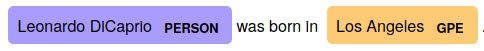
This information can be accessed within spaCy in the following way:

for ent in document.ents:
    print(ent.text, ":", ent.label_)

This piece of code prints the following results:

Leonardo DiCaprio : PERSON
Los Angeles : GPE

Leonardo DiCaprio is well identified as a PERSON. And according to the documentation at https://spacy.io/api/annotation#named-entities, GPE stands for Countries, cities, states; so Los Angles was also identified correctly.

How does that help? Well, now that we have entities, we have node labels:

MATCH (:PERSON {name: "Leonardo DiCaprio"})
MATCH (:GPE {name: "Los Angeles"})

The two preceding Cypher queries can be generated from Python:

for ent in document.ents:
    q = f"MATCH (n:{ent.label_} {{name: '{ent.text}' }})"
    print(q)

In order to identify which relationship we should use to relate the two entities, we are going to use the verb in the sentence:

for token in document:
    if token.pos_ == "VERB":
        print(token.text)

The only printed result will be born, since this is the only verb in our sentence. We can update the preceding code to print the Cypher relationship:

for token in document:
    if token.pos_ == "VERB":
        print(f"[:{token.text.upper()}]")

Putting all the pieces together, we can write a query to check whether the statement is true or not:

MATCH (n0:PERSON {name: 'Leonardo DiCaprio' })
MATCH (n1:GPE {name: 'Los Angeles' })
RETURN EXISTS((n1)-[:BORN]-(n2))

This query returns true if the pattern we are looking for exists in our working graph, and false otherwise.

As you can see, NLP is very powerful and a lot can be done from it if we want to push the analysis further. But the amount of work required is incredibly high, especially if we want to cover several fields (not only people and locations but also gardening products or GitHub repositories). That's the reason why, in the next section, we are going to investigate another possibility enabled by NLP and machine learning: an automatic English to Cypher translator.

Using translation-like models

As you can see from the previous paragraph, natural language understanding helps in automating the human language to a Cypher query, but it relies on some rules. These rules have to be carefully defined and you can imagine how difficult this can be when the number of rules increases. That's the reason why we can also find help in machine learning techniques, especially those related to translation, another part of NLP.

Translation consists in taking a text in a (human) language, and outputting a text in another (human) language, as illustrated in the following diagram, where the translator is a machine learning model, usually relying on artificial neural networks:

The translator's goal is to assign a value (or a vector of values) to each word, this vector carrying the meaning of the word. We will talk about this in more detail in the chapter dedicated to embedding (Chapter 10, Graph Embedding from Graphs to Matrices).

But without knowing the details of the process, can we imagine applying the same logic to translate a human language to Cypher? Indeed, using the same techniques as those used for human language translation, we can build models to convert English sentences (questions) to a Cypher query.

The Octavian-AI company worked on an implementation of such a model in their english2cypher package (https://github.com/Octavian-ai/english2cypher). It is a neural network model implemented with TensorFlow in Python. The model learned from a list of questions regarding the London Tube, together with their translations in Cypher. The training set looks like this:

english: How many stations are between King's Cross and Paddington?

cypher: MATCH (var1) MATCH (var2) 
        MATCH tmp1 = shortestPath((var1)-[*]-(var2))
        WHERE var1.id="c2b8c082-7c5b-4f70-9b7e-2c45872a6de8"
        AND var2.id="40761fab-abd2-4acf-93ae-e8bd06f1e524"
        WITH nodes(tmp1) AS var3
        RETURN length(var3) - 2

Even if we have not yet studied the shortest path methods (see Chapter 4, The Graph Data Science Library and Path Finding), we can understand the preceding query:

1. It starts from getting the two stations mentioned in the question.
2. It then finds the shortest path between those two stations.
3. And counts the number of nodes (stations) in the shortest path.
4. The answer to the question is the length of the path, minus 2 since we do not want to count the start and end station.

But the power of machine learning models lies within their prediction: from a set of known data (the train dataset), they are able to issue predictions for unknown data. The preceding model would, for instance, be able to answer questions such as "How many stations are there between Liverpool Street Station and Hyde park Corner?" even if it has never seen it before.

In order to use such a model within your business, you will have to create a training sample made of a list of English questions with the corresponding Cypher queries able to answer them. This part is similar to the one we performed in the Manually building Cypher queries section. Then you will have to train a new model. If you are not familiar with machine learning and model training, this topic will be covered in more detail in Chapter 8, Using Graph-Based Features in Machine Learning.

You now have a better overview of how graph-based search works and why Neo4j is a good structure to hold the data if user search is an important feature for your company. But knowledge graph applications are not limited to search engines. Another interesting application of the knowledge graph is recommendations, as we will discover now.

Recommendation engine

Recommendations are now unavoidable if you work for an e-commerce website. But e-commerce is not the only use case for recommendations. You can also receive recommendations for people you may want to follow on Twitter, meetups you may attend, or repositories you might like knowing about. Knowledge graphs are a good approach to generate those recommendations.

In this section, we are going to use our GitHub graph to recommend to users new repositories they are likely to contribute to or follow. We will explore several possibilities, split into two cases: either your graph contains some social information (users can like or follow each other) or it doesn't. We'll start from the case where you do not have access to any social data since it is the most common one.

Product similarity recommendations

Recommending products, whether we are talking about movies, gardening tools, or meetups, share some common patterns. Here are some common-sense assertions that can lead to a good recommendation:

• Products in the same categories to a product already bought are more likely to be useful to the user. For instance, if you buy a rake, it probably means you like gardening, so a lawnmower could be of interest to you.
• There are some products that often get bought together, for instance, printers, ink, and paper. If you buy a printer, it is natural to recommend the ink and paper other users also bought.

We are going to see the implementations of those two approaches using Cypher. We will again use the GitHub graph as a playground. The important parts of its structure are shown in the next schema:

It contains the following entities:

• Node labels: User, Repository, Language, and Document
• Relationships:
  • A User node owns or contributes to one or several Repository nodes.
  • A Repository node has one or several Language nodes.
  • A User node can follow another User node.

Thanks to the GitHub API, the USES_LANGUAGE relationship even holds a property quantifying the number of bytes of code using that language.

Products in the same category

In the GitHub graph, we will consider the language as categorizing the repositories. All repositories using Scala will be in the same category. For a given user, we can get the languages used by the repositories they contributed to with the following:

MATCH (:User {login: "boggle"})-[:CONTRIBUTED_TO]->(repo:Repository)-[:USES_LANGUAGE]->(lang:Language)
RETURN lang

If we want to find the other repositories using the same language, we can extend the path from the language node to the other repositories in this way:

MATCH (u:User {login: "boggle"})-[:CONTRIBUTED_TO]->(repo:Repository)-[:USES_LANGUAGE]->(lang:Language)<-[:USES_LANGUAGE]-(recommendation:Repository)
WHERE NOT EXISTS ((u)-[:CONTRIBUTED_TO]->(repo))
RETURN recommendation

For instance, the user boggle contributed to the neo4j repository, which is partly written using Scala. With that technique, we would recommend to this user the repositories neotrients or JUnitSlowTestDiscovery, also using Scala:

However, recommending all repositories using Scala is like recommending all gardening tools because a user bought a rake. It is maybe not accurate enough, especially when the categories contain lots of items. Let's see which other kinds of methods can be used to improve this technique.

Products frequently bought together

One possible solution is to trust your users. Information about their behavior is also valuable.

Consider the pattern in the following diagram:

The user boggle contributed to the repository neo4j. Three more users contributed to it, and also contributed to the repositories parents and neo4j.github.com. Maybe boggle would be interested in contributing to one of those repositories:

MATCH (user:User {login: "boggle"})-[:CONTRIBUTED_TO]->(common_repository:Repository)<-[:CONTRIBUTED_TO]-(other_user:User)-[:CONTRIBUTED_TO]->(recommendation:Repository)
WHERE user <> other_user
RETURN recommendation

We can even group together this method and the preceding one, by selecting only repositories using a language the user knows and with at least one common contributor:

MATCH (user:User {login: "boggle"})-[:CONTRIBUTED_TO]->(common_repository:Repository)<-[:CONTRIBUTED_TO]-(other_user:User)-[:CONTRIBUTED_TO]->(recommendation:Repository)
MATCH (common_repository)-[:USES_LANGUAGE]->(:Language)<-[:USES_LANGUAGE]-(recommendation)
WHERE user <> other_user
RETURN recommendation

When having only a few matches, we can afford to display all returned items. But if your database grows, you will find a lot of possible recommendations. In that case, finding a way to rank the recommended items would be essential.

Recommendation ordering

If you look again at the preceding image, you can see that the repository neo4j.github.com is shared between two people, while the parents repository would be recommended by only one person. This information can be used to rank the recommendations. The corresponding Cypher query would be as follows:

MATCH (user:User {login: "boggle"})-[:CONTRIBUTED_TO]->(common_repository:Repository)<-[:CONTRIBUTED_TO]-(other_user:User)-[:CONTRIBUTED_TO]->(recommendation:Repository)
WHERE user <> other_user
WITH recommendation, COUNT(other_user) as reco_importance
RETURN recommendation
ORDER BY reco_importance DESC
LIMIT 5

The new WITH clause is introduced to perform the aggregation: for each possible recommended repositories, we count how many users would recommend it.

This is the first way of using user data to provide accurate recommendations. Another way is, when possible, to take into account using social relationships, as we will see now.

Social recommendations

If your knowledge graph contains data related to social links between users, like GitHub or Medium does, a brand new field of recommendations is open to you. Because you know which person a given user likes or follows, you can have a better idea about which type of content this user is likely to appreciate. For instance, if someone you follow on Medium claps a story, it is much more likely you will also like it, compared to any other random story you can find on Medium.

Luckily, we have some social data in our GitHub knowledge graph, through the FOLLOWS relationships. So will use this information to provide other recommendations to our users.

Products bought by a friend of mine

If we want to recommend new repositories to our GitHub users, we can think of the following rule: repositories of a user I follow are more likely to be of interest to me, otherwise I wouldn't follow those users. We can use Cypher to identify those repositories:

MATCH (u:User {login: "mkhq"})-[:FOLLOWS]->(following:User)-[:CONTRIBUTED_TO]->(recommendation:Repository)
WHERE NOT EXISTS ((u)-[:CONTRIBUTED_TO]->(recommendation))
RETURN DISTINCT recommendation

This query matches patterns similar to the following one:

We can also use recommendation ordering here. The higher the number of people I follow that also contributed to a given repository, the higher the probability that I will also contribute to it. This translates into Cypher in the following way:

MATCH (u:User {login: "mkhq"})-[:FOLLOWS]->(following:User)-[:CONTRIBUTED_TO]->(recommendation:Repository)
WHERE NOT EXISTS ((u)-[:CONTRIBUTED_TO]->(recommendation))
WITH user, recommendation, COUNT(following) as nb_following_contributed_to_repo
RETURN recommendation
ORDER BY nb_following_contributed_to_repo DESC
LIMIT 5

The first part of the query is exactly the same as the previous one, while the second part is similar to the query we wrote in the previous section: for each possible recommendation, we count how many users mkhg is following would recommend it.

We have seen several ways of finding recommendations based on pure Cypher. They can be extended depending on your data: the more information you have about your products and customers, the more precise the recommendations can be. In the following chapters, we will discover algorithms to create clusters of nodes within the same community. This concept of community can also be used in the context of recommendations, assuming users within the same community are more likely to like or buy the same products. More details will be given in Chapter 7, Community Detection and Similarity Measures.

Summary

This chapter described in detail how to create a knowledge graph, either using already structured data, such as an API result, or an existing knowledge graph that can be queried, such as Wikidata. We also learned how to use NLP and named entity recognition in order to extract information from unstructured data, such as a human-written text, and turn this information into a structured graph. We have also learned about two important applications of knowledge graphs: graph-based search, the method used by Google to provide even more accurate results to the users, and recommendations, which are a mandatory step for e-commerce today.

All of this was done with Cypher, extended by some plugins such as APOC or the NLP GraphAware plugin. In the rest of this book, we will make extensive use of another very important library when dealing with graph analytics: the Neo4j Graph algorithms library. The next chapter will introduce it and give application examples in the context of the shortest pathfinder challenges.

Questions

Using Wikidata, what kind of contextual information can we add to the repository language?

Further reading

• If you are new to NLP and want to learn more about it, you can start with Natural Language Processing Fundamentals, D. Gunning and S. Ghosh, Packt Publishing.

• Then, consider checking out Hands-On Natural Language Processing with Python, R. Shanmugamani and R. Arumugam, Packt Publishing.
• W3C specifications:
• RDF: https://www.w3.org/TR/rdf-concepts/
• SPARQL: https://www.w3.org/TR/rdf-sparql-query/
• Neural Machine Translation models used by Google Translate:
• The initial paper by Google: https://research.google/pubs/pub45610/ 
• The implementation using Tensorflow: https://github.com/tensorflow/nmt