In this chapter, we are going to talk about node importance, also known as centrality algorithms. As you will discover, several techniques have been developed, based on the definition of importance for a given graph and a given problem. We will learn about the most famous techniques, starting with degree centrality and the PageRank algorithm used by Google. For the latter, we will go through an example implementation and run it on a simple graph to fully understand how it works and when it can be used. After discovering the other types of centrality algorithms, such as betweenness centrality, we will conclude this chapter with explanations of how centrality algorithms can be used in the context of fraud detection. In this example, we will use, for the first time, the tools provided in the GDS to create a projected graph from Cypher in order to create fake relationships between nodes to meet analysis needs.
The following topics will be covered in this chapter:
- Defining importance
- Computing degree centrality
- Understanding the PageRank algorithm
- Path-based centrality metrics
- Applying centrality to fraud detection
Let's get started!
Technical requirements
In this chapter, we will use the following tools:
- The Neo4j graph database with the Graph Data Science Library
- The code files for this chapter, which are available at https://github.com/PacktPublishing/Hands-On-Graph-Analytics-with-Neo4j/tree/master/ch6
If you are using Neo4j < 4.0, then the latest compatible version of the GDS plugin is 1.1, whereas if you are using Neo4j ≥ 4.0, then the first compatible version of the GDS plugin is 1.2.
Defining importance
Determining the most important node of a graph depends on your definition of importance. This definition itself depends on the goal you are trying to achieve. In this chapter, we will study two examples of importance:
- Information spread within a social network
- Critical nodes in a road or computer network
We will learn that each of these problems can be tackled with centrality algorithms. In this section, we will consider the following graph as an example to help us understand the different definitions of importance:

Which node is the most important in this network? The answer depends on what important means in a given context. Let's consider the different ways of defining importance.
Popularity and information spread
The most obvious way to define importance is with the influencer concept. Most influential nodes have many connections and, as such, are well placed to spread information. In the context of social networks, influencers often get offered advertising contracts with brands that want to harness their influencing power and let as many people as possible know about their products. With this in mind, nodes 3, 5, 6, and 9 in the previous diagram all have three connections, making them the most important nodes.
To go further and try to disentangle these four nodes, other methods have been proposed. The most famous of them is the PageRank algorithm, used by Google to rank the results of its search engine. PageRank updates the importance of a given node, taking into account the importance of its neighbors. If a web page has backlinks from an important page, its importance will increase, compared to another page that is referenced by less important pages.
These methods, based on degrees, have many applications, from influencing to fraud detection. But if you are looking for a critical node in a road or computer network, for instance, they are not the most well-suited methods.
Critical or bridging nodes
Degree-based centrality algorithms identify important nodes in terms of their connections. But what happens to our graph if node 5 disappears? We end up with three disconnected components:
- Nodes 1, 2, 3, and 4
- Nodes 6, 7, and 8
- Nodes 9, 10, and 11
This new layout is illustrated in the following diagram:

As you can see, communication from one component to another will be completely impossible. Consider, for instance, nodes 1 and 10. There is no possible path between them anymore. In a telecommunication or road network, this situation can have serious consequences, from huge traffic jams to the impossibility of calling emergency services. It needs to be avoided at any cost, meaning that nodes such as node 5 in our test graph need to be identified in order to be better protected. For this reason, node 5 is called a critical (or bridging) node.
Fortunately, we have centrality algorithms to measure this kind of importance. We will group them together under the path-based category. The closeness and betweenness centrality algorithms, which we will look at later in this chapter, are part of this category.
In the next two sections, we are going to detail degree centrality and the PageRank algorithm. The following section will be more focused on two examples of path-based centrality: closeness and betweenness.
Computing degree centrality
Computing degree centrality involves sorting nodes based on how many relationships they have. This can be computed with base Cypher or invoked via the GDS plugin and a projected graph.
Formula
Degree centrality Cn is defined as follows:
Cn = deg(n)
Here, deg(n) denotes the number of edges connected to the node n.
If your graph is directed, then you can define the incoming and outgoing degree as the number of relationships starting from node n and the number of relationships ending in n, respectively.
For instance, let's consider the following graph:

Node A has one incoming relationship (coming from B) and two outgoing relationships (to B and D), so its incoming degree is 1 and its outgoing degree is 2. The degrees of each node are summarized in the following table:
| Node | Outgoing degree | Incoming degree | Degree (undirected) |
| A | 2 | 1 | 3 |
| B | 1 | 3 | 4 |
| C | 1 | 0 | 1 |
| D | 1 | 1 | 2 |
Let's now see how to get these results in Neo4j. You can create this small graph using the following Cypher statement:
CREATE (A:Node {name: "A"})
CREATE (B:Node {name: "B"})
CREATE (C:Node {name: "C"})
CREATE (D:Node {name: "D"})

CREATE (A)-[:LINKED_TO {weight: 1}]->(B)
CREATE (B)-[:LINKED_TO]->(A)
CREATE (A)-[:LINKED_TO]->(D)
CREATE (C)-[:LINKED_TO]->(B)
CREATE (D)-[:LINKED_TO]->(B)
Computing degree centrality in Neo4j
Counting the number of edges connected to a node with Neo4j is possible using only Cypher and aggregation functions. For instance, the following query counts the number of outgoing relationships from each node:
MATCH (n:Node)-[r:LINKED_TO]->()
RETURN n.name, count(r) as outgoingDegree
ORDER BY outgoingDegree DESC
Running this query on the small graph we studied in the previous section gives us the following result:
╒══════════╤════════════════╕
│"nodeName"│"outgoingDegree"│
╞══════════╪════════════════╡
│"A"       │2               │
├──────────┼────────────────┤
│"B"       │1               │
├──────────┼────────────────┤
│"C"       │1               │
├──────────┼────────────────┤
│"D"       │1               │
└──────────┴────────────────┘
The incoming degree can also be computed using a slightly modified Cypher query, where the direction of the relationship is reversed thanks to the use of the <-[]- notation (instead of -[]->):
MATCH (n:Node)<-[r:LINKED_TO]-()
RETURN n.name as nodeName, count(r) as incomingDegree
ORDER BY incomingDegree DESC
The results of this query are reported in the following table:
╒══════════╤════════════════╕
│"nodeName"│"incomingDegree"│
╞══════════╪════════════════╡
│"B"       │3               │
├──────────┼────────────────┤
│"A"       │1               │
├──────────┼────────────────┤
│"D"       │1               │
└──────────┴────────────────┘
As you can see, the centrality result is missing from node C, which is not connected to any other node. This can be fixed using OPTIONAL MATCH, like this:
MATCH (n:Node)
OPTIONAL MATCH (n)<-[r:LINKED_TO]-()
RETURN n.name as nodeName, count(r) as incomingDegree
ORDER BY incomingDegree DESC
This time, the result contains node C:
╒══════════╤════════════════╕
│"nodeName"│"incomingDegree"│
╞══════════╪════════════════╡
│"B"       │3               │
├──────────┼────────────────┤
│"A"       │1               │
├──────────┼────────────────┤
│"D"       │1               │
├──────────┼────────────────┤
│"C"       │0               │
└──────────┴────────────────┘
However, it is much more convenient to use the GDS implementation, which already takes care of these components.
Computing the outgoing degree using GDS
When using GDS, we need to define the projected graph. In this case, we can use the simplest syntax since we want to add all the nodes and all their relationships in their natural direction:
CALL gds.graph.create("projected_graph", "Node", "LINKED_TO")
Then, we can use this projected graph to run the degree centrality algorithm:
CALL gds.alpha.degree.stream("projected_graph")
YIELD nodeId, score
RETURN gds.util.asNode(nodeId).name as nodeName, score
ORDER BY score DESC
The result of this query is reproduced here:
╒══════════╤═══════╕
│"nodeName"│"score"│
╞══════════╪═══════╡
│"A"       │2.0    │
├──────────┼───────┤
│"B"       │1.0    │
├──────────┼───────┤
│"C"       │1.0    │
├──────────┼───────┤
│"D"       │1.0    │
└──────────┴───────┘
If you want to compute the incoming degree instead, you have to change the definition of the projected graph.
Computing the incoming degree using GDS
In GDS, we need to define a projected graph, which we can name (and save for future use in the same session) or keep unnamed.
Using a named projected graph
Creating a projected graph that will have all the relationships in the reverse direction requires a detailed configuration for the relationship's orientation:
CALL gds.graph.create(
    "projected_graph_incoming",
    "Node",
    {
        LINKED_TO: {
            relationship: "LINKED_TO",
            orientation: "REVERSE"
        }
    }
)
This new projected graph (projected_graph_incoming) contains the nodes with the Node label. It will also have relationships that are of the LINKED_TO type, which will be copies of the LINKED_TO relationships from the original graph but in the REVERSE direction. In other words, if the original graph contains the (A)-[:LINKED_TO]->(B) relationship, then the projected graph will only contain the (B)-[:LINKED_TO]->(A) pattern. You can run the degree centrality algorithm on this new projected graph with the following query:
CALL gds.alpha.degree.stream("projected_graph_incoming")
YIELD nodeId, score
RETURN gds.util.asNode(nodeId).name as name, score
ORDER BY score DESC
Here are the results:
╒══════════╤═══════╕
│"nodeName"│"score"│
╞══════════╪═══════╡
│"B"       │3.0    │
├──────────┼───────┤
│"A"       │1.0    │
├──────────┼───────┤
│"D"       │1.0    │
├──────────┼───────┤
│"C"       │0.0    │
└──────────┴───────┘
If your graph is undirected, you will have to use the orientation: "UNDIRECTED" parameter in the projected graph definition, as we did in the chapters dedicated to the shortest path (Chapter 4, The Graph Data Science Library and Path Finding) and spatial data (Chapter 5, Spatial Data).
Using an anonymous projected graph
GDS also gives us the option to run an algorithm without a named projected graph. In this case, the projected graph will be generated on the fly when calling the GDS procedure. For instance, in order to get the node degree for an undirected graph, you can use the following code:
CALL gds.alpha.degree.stream(
    {
        nodeProjection: "Node",
        relationshipProjection: {
            LINKED_TO: {
                type: "LINKED_TO",
                orientation: "UNDIRECTED"
            }
        }
    }
) YIELD nodeId, score
RETURN gds.util.asNode(nodeId).name as nodeName, score
ORDER BY score DESC
This query returns the following results:
╒══════════╤═══════╕
│"nodeName"│"score"│
╞══════════╪═══════╡
│"B"       │4.0    │
├──────────┼───────┤
│"A"       │3.0    │
├──────────┼───────┤
│"D"       │2.0    │
├──────────┼───────┤
│"C"       │1.0    │
└──────────┴───────┘
This closes this section on degree centrality calculations with Neo4j. However, as we discussed in the first section of this chapter, degree centrality can be improved to take into account the quality of each connection. This is what the PageRank algorithm is trying to achieve, as we will discover now.
Understanding the PageRank algorithm
The PageRank algorithm is named after Larry Page, one of the co-founders of Google. The algorithm was developed back in 1996 in order to rank the results of a search engine. In this section, we will understand the formula by building it step by step. We will then run the algorithm on a single graph to see how it converges. We will also implement a version of the algorithm using Python. Finally, we will learn how to use GDS to get this information from a graph stored in Neo4j.
Building the formula
Let's consider PageRank in the context of the internet. The PageRank algorithm relies on the idea that not all incoming links have the same weight. As an example, consider a backlink from a New York Times article to an article in your blog. It is more important than a link from a website that gets 10 visits a month since it will redirect more users to your blog. So, we would like the New York Times to have more weight than the low-traffic website. The challenge here is to assess the weight of an incoming connection. In the PageRank algorithm, this weight is the importance of the page or the rank of the page. So, we end up with a recursive formula where each page's importance is measured compared to the other pages:
PR(A) = PR(N1) + ... + PR(Nn)
Here, Ni (i=1...n) is the pages pointing to page A (the incoming relationships).
This is not the final formula for PageRank. Two other aspects need to be taken into account. First, we will balance the importance of an incoming link for pages that have many outgoing links. It is as if each page has an equal number of votes to distribute to others. It can give all its votes to one single page, in which case the link is very strong, or share them among many pages, giving many links less importance.
So, we can update the PageRank formula like this:
PR(A) = PR(N1)/C(N1) + ... + PR(Nn)/C(Nn)
Here, C(Ni) is the number of outgoing links from Ni.
The second aspect to integrate to finally get to the PageRank formula is the damping factor. It requires some more explanation and will be covered in the following subsection.
The damping factor
Last but not least, the PageRank algorithm introduces a damping factor to mitigate the effect of the neighbors. The idea is that, when navigating from one page to another, the internet user usually clicks on links. But in some cases, the user might become bored or, for whatever reason, go to another page. The probability of this happening is modeled by the damping factor. The final PageRank formula from the initial paper is as follows:
PR(A) = (1 - d) + d * (PR(N1)/C(N1) + ... + PR(Nn)/C(Nn))
Usually, the damping factor d is set to be around 0.85, meaning the probability of a user randomly navigating to a page without following a link is 1 - d = 15%.
Another important effect of the damping factor is visible for nodes with no outgoing links, also called sinks. Without the damping factor, these nodes will have the tendency to take the rank given by their neighbors without giving it back, breaking the principle of the algorithm.
Normalization
Although the previous formula is the one from the original paper, which introduced the PageRank algorithm in 1996, be aware that another one is sometimes used instead. In the original formula, the sum of ranks for all nodes adds up to N, which is the number of nodes. The updated formula is normalized to 1 instead of N and is written as follows:
PR(A) = (1 - d) / N + d * (PR(N1)/C(N1) + ... + PR(Nn)/C(Nn))
You can understand this easily by assuming that the ranks for all the nodes are initialized to 1/N. Then, at each iteration, each node will equally distribute this rank to all its neighbors so that the sum remains constant.
This formula was chosen for the PageRank implementation in networkx, the Python package for graph manipulation. However, Neo4j GDS uses the original formula. For this reason, in the following subsections, we are going to use the original version of the PageRank equation.
Running the algorithm on an example graph
The PageRank algorithm can be implemented with an iterative process where, at each iteration, the rank of a given node is updated based on the rank of its neighbors in the previous iteration. This process is repeated until the algorithm converges, meaning that the PageRank difference between two iterations is lower than a certain threshold. In order to understand how it works, we are first going to run it manually on the simple graph we studied in the Degree centrality section.
In order to compute PageRank, we need an outgoing degree for each node, which is simply the number of arrows starting from the node. In the graph illustrated in the preceding diagram, these degrees are as follows:
A => 2
B => 1
C => 1
D => 1
In order to run the PageRank algorithm (in its iterative form), we need to give an initial value to the rank of each node. Since we do not have any a priori preference for a given node, we can initialize these values with the uniform value of 1. Note that this initialization preserves the PageRank algorithm's normalization: the sum of PageRank in its initial state is still equal to N, which is the number of nodes.
Then, during iteration 1, the page rank values are updated as follows:
- Node A: Receives one incoming connection from node B, so its updated PageRank is as follows:
new_pr_A = (1 - d) + d * (old_pr_B / out_deg_B)
         = 0.15 + 0.85 * (1 / 1)
= 1.0 - Node B: Has three incoming connections:
- One coming from A
- One coming from C
- And a final one coming from D
So, its page rank is updated with the following:
   new_pr_B = (1 - d)
            + d * (old_pr_A / out_deg_A
                 + old_pr_C / out_deg_C
                 + old_pr_D / out_deg_D)
         = 0.15 + 0.85 * (1 / 2 + 1 / 1 + 1 / 1)
         = 2.275
- Node C: Has no incoming connection, so its rank is updated with the following:
new_pr_C = (1 - d)
= 0.15 - Node D: Receives one connection from A:
new_pr_D = (1 - d) + d * (old_pr_A / out_deg_A)
         = 0.15 + 0.85 * (1 /2)
         = 0.575
Iteration 2 consists of repeating the same operation but changing the old_pr values. For instance, the updated PageRank of node B after iteration 2 would be as follows:
new_pr_B = (1 - d) + d * (old_pr_A / out_deg_A + old_pr_C / out_deg_C + old_pr_D / out_deg_D)
         = 0.15 + 0.85 * (1.0 / 2 + 0.15 / 1 + 0.575 / 1)
         = 1.191
The rank of B in the second iteration decreases a lot, while the rank of A increases from 0.575 to 1.117.
The first three iterations are summarized in the following table:
| Iteration/Node | A | B | C | D |
| Initialization | 1 | 1 | 1 | 1 |
| 0 | 1.0 | 2.275 | 0.15 | 0.575 |
| 1 | 2.084 | 1.191 | 0.15 | 0.575 |
| 2 | 1.163 | 1.652 | 0.15 | 1.036 |
The question of when to stop iterating will be answered in the following subsection, where we are going to implement a version of PageRank using Python.
Implementing the PageRank algorithm using Python
In order to implement the PageRank algorithm, we need to agree on a graphical representation. In order to avoid introducing other dependencies, we will use a simple representation via dictionaries. Each node in the graph will have a key in the dictionary. The associated value contains another dictionary whose keys are the linked nodes from the key. The graph we are studying in this section is written as follows:
G = {
    'A': {'B': 1, 'D': 1},
    'B': {'A': 1},
    'C': {'B': 1},
    'D': {'B': 1},
}
The page_rank function we are going to write has the following parameters:
- G, the graph for which the algorithm will compute the PageRank.
- d, the damping factor whose default value is 0.85.
- tolerance, the tolerance to stop the iteration when the algorithm has converged. We will set a default value of 0.01.
- max_iterations, a sanity check to make sure we do not loop infinitely in case the algorithm fails to converge. As an order of magnitude, in the initial PageRank publication, the authors reported that the convergence was reached after around 50 iterations, for a graph containing more than 300 million edges.
Here is the function definition:
def page_rank(G, d=0.85, tolerance=0.01, max_iterations=50):
Then, we need to initialize the PageRank. Similar to the previous section, we assign a value of 1 to all nodes, since we do not have any a priori belief about the final result:
pr = dict.fromkeys(G, 1.0)
We also compute the number of outgoing links for each node, since this will be used later on. With our definition of the graph G, the number of outgoing links is just the length of the dictionary associated with each key:
outgoing_degree = {k: len(v) for k, v in G.items()}
Now that we have initialized all the variables we need, we can start the iterative process, where we will have max_iter iterations at most. At each iteration, we will save the pr dictionary from the previous iteration into the old_pr dictionary and create a new pr dictionary, initialized to 0, that will be updated each time we find an incoming relationship to the node so that old_pr finally contains the updated pr for each node:
for it in range(max_itererations):
        print("======= Iteration", it)
        old_pr = dict(pr)
        pr = dict.fromkeys(pr.keys(), 0)
The next step is to iterate over each node of the graph and update its rank with the fixed (1-d)/N term and one of its neighbors:
for node in G:
            for neighbor in G[node]:
                pr[neighbor] += d * old_pr[node] / outgoing_degree[node]
            pr[node] += (1 - d)
        print("New PR:", pr)
Finally, after this iteration on each node, we can compare the pr dictionary from the previous iteration (old_pr) and the new one (pr). If the mean of the differences is below the tolerance threshold, the algorithm has converged and we can return the current pr values:
# check convergence
        mean_diff_to_prev_pr = sum([abs(pr[n] - old_pr[n]) for n in G]) / len(G)
        if mean_diff_to_prev_pr < tolerance:
            return pr
Finally, we can call this newly created function on the graph we defined earlier:
pr = page_rank(G)
This gives us the following output after the ninth iteration:
{'A': 1.50, 'B': 1.57, 'C': 0.15, 'D': 0.78}
This implementation is useful for understanding the algorithm, but that's its only purpose. When using the PageRank algorithm in a real-life application, you will have to rely on optimized and tested solutions, such as the one implemented in the GDS plugin for Neo4j.
Using GDS to assess PageRank centrality in Neo4j
As usual, when using GDS, we need to define the projected graph that will be used to run the algorithm. In this example, we will run the PageRank algorithm on the directed graph, which is the default behavior of projected graphs. If you didn't do so in the previous section, you can use the following query to create the named projected graph out of the nodes with a Node label and relationships with the LINKED_TO type:
CALL gds.graph.create("projected_graph", "Node", "LINKED_TO")
We can then run the PageRank algorithm on this projected graph. The signature of the PageRank procedure in Neo4j is as follows:
CALL gds.pageRank(<projected_graph_name>, <configuration>)
The configuration map accepts the following parameters:
- dampingFactor: A float between 0 and 1 corresponding to the damping factor (d, in our Python implementation). The default value is 0.85.
- maxIterations: The maximum number of iterations (the default is 20).
- tolerance: The tolerance to measure convergence (the default is 1E-7).
When using default values for all parameters, we can run the PageRank algorithm and stream the results with the following Cypher statement:
CALL gds.pageRank.stream("projected_graph", {}) YIELD nodeId, score
RETURN gds.util.asNode(nodeId).name as nodeName, score
ORDER BY score DESC
The streamed results are comparable to the ones we obtained earlier in this chapter with a custom implementation, even if they're not strictly identical.
Comparing degree centrality and the PageRank results
In order to understand what PageRank is doing, let's compare the results of degree centrality and the PageRank algorithms on our small directed graph. This comparison is shown in the following table:
| Node | Degree centrality | PageRank centrality |
| A | 2 | 1.44 |
| B | 1 | 1.52 |
| C | 1 | 0.15 |
| D | 1 | 0.76 |
While node A has the highest outgoing degree (2), it receives only one link, meaning only one other page in the graph trusts it. On the other hand, node B has an outgoing degree of 1, but three other pages of the network are pointing to it, giving it more credibility. That's the reason why, with PageRank centrality, the most important node is now node B.
Variants
Depending on the desired goal, PageRank has several variants. These are also implemented in GDS.
ArticleRank
ArticleRank is a variant of PageRank whereby the chance of assuming that a link coming from a page with a few outgoing links is more important than others is smaller. This is achieved by introducing the average degree in the formula:
AR(A) = (1 - d) + d * (AR(N1)/(C(N1) + AVG(C)) + ... + AR(Nn)/(C(Nn) + AVG(C)))
Here, AVG(C) is the average number of outgoing connections for all pages in the network.
Usage within GDS is similar to that of PageRank:
CALL gds.alpha.articleRank.stream("projected_graph", {})
YIELD nodeId, score
RETURN gds.util.asNode(nodeId).name as name, score
ORDER BY score DESC
However, the results, as shown here, are much closer to each other:
╒══════════╤═══════╕
│"nodeName"│"score"│
╞══════════╪═══════╡
│"B"       │0.37   │
├──────────┼───────┤
│"A"       │0.29   │
├──────────┼───────┤
│"D"       │0.23   │
├──────────┼───────┤
│"C"       │0.15   │
└──────────┴───────┘
Personalized PageRank
In personalized PageRank, more weight is given to some user-defined nodes. For instance, giving a higher importance to node C can be achieved with this query:
MATCH (A:Node {name: "A"})
CALL gds.pageRank.stream("projected_graph", {
  sourceNodes: [A]
})
YIELD nodeId, score
RETURN gds.util.asNode(nodeId).name AS nodeName, round(score*100)/100 as score
ORDER BY score DESC
The results are listed in the following table. You can see that node A has gained more importance than it did in the traditional PageRank:
╒══════════╤═══════╕
│"nodeName"│"score"│
╞══════════╪═══════╡
│"A"       │0.44   │
├──────────┼───────┤
│"B"       │0.34   │
├──────────┼───────┤
│"D"       │0.19   │
├──────────┼───────┤
│"C"       │0.0    │
└──────────┴───────┘
Applications of personalized PageRank include recommendations, where we already have some prior knowledge about the products a given customer might like based on their previous purchases.
Eigenvector centrality
PageRank is actually a variant of another centrality metric called eigenvector centrality. Let me introduce some math here by rebuilding the PageRank formula using matrices.
The adjacency matrix
To work on a graph and simulate information spread within it, we need a way to model the complex relationship pattern. The simplest way of doing so is to build the adjacency matrix of the graph. It is a 2D array where the element on line i and column j is equal to 1 if there is an edge going from node i to node j and 0 otherwise.
The adjacency matrix of the graph we studied during the implementation of the PageRank algorithm is as follows:

The first element of the first row corresponds to the edge between A and A. Since A is not connected to itself, this element is 0. The second element of the first row holds information about the edge between A and B. Since there is a relationship between these two nodes, this element is equal to 1. Similarly, the second row of the adjacency matrix contains information about the outgoing edges from node B. This node has a single outgoing edge going to A. A corresponds to the first column of the matrix, so only the first element of the second row is 1.
Lots of information can be extracted from this matrix. For instance, we can find the outgoing degree of each node by summing the values in a given row and the incoming degree by summing the values in a given column.
The adjacency matrix with normalized rows is as follows:

PageRank with matrix notation
Now, let's consider that node A contains a value that we want to propagate to its neighbors. We can find how the value will be propagated through the graph with a simple dot product:

This is what happens if all the initial values are initialized to 1:
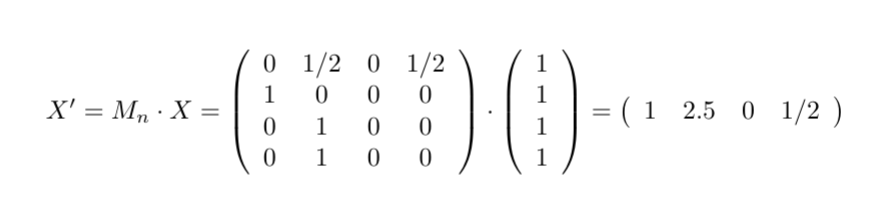
We are almost there. The only missing part to retrieving the PageRank formula is the damping factor d:

As you can see, we are getting the same values that we found in the previous sections. With this formalism, finding the rank of each node is equivalent to solving the following equation:
X' = (1-d) + d * M_n * X = X
In this equation, the values of the X vector are the PageRank centralities for each node.
Now, let's go back to eigenvector centrality.
Eigenvector centrality
Finding eigenvector centrality involves solving a similar but simpler equation:
M.X = λ.X
Here, M is the adjacency matrix. In mathematical terms, this means finding the eigenvectors of this adjacency matrix. There might be several possible solutions with different values for λ (the eigenvalues), but the constraint that the centrality for each node must be positive only leaves one single solution – eigenvector centrality.
Due to its similarity with PageRank, its use cases are also similar: use eigenvector centrality when you want a node's importance to be influenced by the importance of its neighbors.
Computing eigenvector centrality in GDS
Eigenvector centrality is implemented in GDS. You can compute it on your favorite projected graph using the following code:
CALL gds.alpha.eigenvector.stream("projected_graph", {}) YIELD nodeId, score as score
RETURN gds.util.asNode(nodeId).name as nodeName, score
ORDER BY score DESC
This closes a long section about the PageRank algorithm and its variants. However, as we discussed earlier, node importance is not necessarily related to popularity. In the next section, we are going to talk about other centrality algorithms, such as betweenness centrality, which can be used to identify the critical nodes in a network.
Path-based centrality metrics
As we discussed in the first section of this chapter (Defining importance), the neighborhood approach is not the only way to measure importance. Another approach is to use a path within the graph. In this section, we will discover two new centrality metrics: closeness and betweenness centrality.
Closeness centrality
Closeness centrality measures how close a node is, on average, to all the other nodes in the graph. It can be seen as centrality from a geometrical point of view.
Normalization
The corresponding formula is as follows:
Cn = 1 / ∑ d(n, m)
Here, m denotes all the nodes in the graph that are different from n, and d(n, m) is the distance of the shortest path between n and m.
A node that is, on average, closer to all other nodes will have a low ∑ d(n, m), resulting in high centrality.
Closeness centrality prevents us from comparing values across graphs with different numbers of nodes since graphs with more nodes will have more terms in the sum and hence lower centrality by construction. To overcome this issue, normalized closeness centrality is used instead:
Cn = (N-1) / ∑ d(n, m)
This is the formula that's selected for GDS.
Computing closeness from the shortest path algorithms
In order to understand how closeness is computed, let's compute it manually using the shortest path procedures of GDS. In Chapter 4, The Graph Data Science Plugin and Path Finding, we discovered the Single Source Shortest Path algorithm (deltastepping), which can compute the shortest path between a given start node and all the other nodes in the graph. We are going to use this procedure to find the sum of distances from one node to all others, and then infer centrality.
To do so, we are going to use the undirected version of the test graph we used in the Understanding the PageRank algorithm section. To create the projected graph, use the following query:
CALL gds.graph.create("projected_graph_undirected_weight", "Node", {
          LINKED_TO: {
            type: "LINKED_TO",
            orientation: "UNDIRECTED",
            properties: {
                  weight: {
                    property: "weight",
                    defaultValue: 1.0
                  }
            }
        }
    }
)
On top of using the undirected version of our graph, we also add a weight property to each relationship, with a default value of 1.
We can then call the SSSP algorithm with a query like this:
MATCH (startNode:Node {name: "A"})
CALL gds.alpha.shortestPath.deltaStepping.stream(
    "projected_graph_undirected_weight",
    {
        startNode: startNode,
        delta: 1,
        relationshipWeightProperty: 'weight'
    }
) YIELD nodeId, distance
RETURN gds.util.asNode(nodeId).name as nodeName, distance
Now, you can check that the distances are correct. Starting from here, we can apply the closeness centrality formula:
MATCH (startNode:Node)
CALL gds.alpha.shortestPath.deltaStepping.stream(
    "projected_graph_undirected_weight",
    {
        startNode: startNode,
        delta: 1,
        relationshipWeightProperty: 'weight'
    }
) YIELD nodeId, distance
RETURN startNode.name as node, (COUNT(nodeId) - 1)/SUM(distance) as d
ORDER BY d DESC
Here are the results:
╒══════╤════╕
│"node"│"d" │
╞══════╪════╡
│"B"   │1.0 │
├──────┼────┤
│"A"   │0.75│
├──────┼────┤
│"D"   │0.75│
├──────┼────┤
│"C"   │0.6 │
└──────┴────┘
In terms of closeness, B is the most important node, which is expected since it is linked to all the other nodes in the graph.
We managed to get the closeness centralities using the SSSP procedure, but there is a much simpler way to get the closeness centrality results from GDS.
The closeness centrality algorithm
Fortunately, closeness centrality is implemented as a standalone algorithm within GDS. We can directly get closeness centralities for each node with the following query:
CALL gds.alpha.closeness.stream("projected_graph_undirected_weight", {})
YIELD nodeId, centrality as score
RETURN gds.util.asNode(nodeId).name as nodeName, score
ORDER BY score DESC
Closeness centrality in multiple-component graphs
Some graphs are made of several components, meaning some nodes are totally disconnected from others. This was the case for the US states graph we built in Chapter 2, The Cypher Query Language, because some states do not share borders with any other state. In such cases, the distance between nodes in two disconnected components is infinite and the centrality of all the nodes drops to 0. Because of that, the centrality algorithm in GDS implements a slightly modified version of the closeness centrality formula, where the sum of distances is performed over all the nodes in the same component. In the next chapter, Chapter 7, Community Detection and Similarity Measures, we will discover how to find nodes belonging to the same component.
In the next section, we are going to learn about another way to measure centrality using a path-based technique: betweenness centrality.
Betweenness centrality
Betweenness is another way to measure centrality. Instead of summing the distances, we are now counting the number of shortest paths traversing a given node:
Cn = ∑ σ(u, v | n) / ∑ σ(u, v)
Here, σ(u, v) is the number of shortest paths between u and v, and σ(u, v | n) is the number of such paths passing through n.
This measure is particularly useful for identifying critical nodes in a network, such as bridges in a road network.
It is used in the following way with GDS:
CALL gds.alpha.betweenness.stream("projected_graph", {})
YIELD nodeId, centrality as score
RETURN gds.util.asNode(nodeId).name, score
ORDER BY score DESC
gds.betweenness.stream and gds.betweenness.write.
Here are the sorted betweenness centralities for our test graph:
╒══════════╤═══════╕
│"nodeName"│"score"│
╞══════════╪═══════╡
│"B"       │3.0    │
├──────────┼───────┤
│"A"       │2.0    │
├──────────┼───────┤
│"C"       │0.0    │
├──────────┼───────┤
│"D"       │0.0    │
└──────────┴───────┘
As you can see, B is still the most important node. But the importance of node D has decreased because none of the shortest paths between two pairs of nodes go through D.
We have now studied many different types of centrality metrics. Let's try and compare them on the same graph to make sure we understand how they work and which metric to use in which context.
Comparing centrality metrics
Let's go back to the graph we started analyzing in the first section. The following diagram shows a comparison of several of the centrality algorithms we studied in this chapter:

If degree centrality can't differentiate between four nodes that all have three connections (nodes 3, 5, 6, and 9), PageRank is able to make some nodes stand out from the crowd by giving more importance to nodes 3 and 6. Closeness and betweenness both clearly identify node 5 as the most critical: if this node disappears, the paths within the graph will be completely changed or even impossible, as we discussed in the first section of this chapter.
Centrality algorithms have many types of applications. In the next section, we will review some of them, starting from the fraud detection use case.
Applying centrality to fraud detection
Fraud is one of the major sources of loss for private companies, as well as public institutions. It takes many different forms, from duplicating user accounts to insurance or credit card fraud. Of course, depending on the type of fraud you are interested in, solutions for identifying fraudsters will vary. In this section, we are going to review the different types of fraud and how a graph database such as Neo4j can help in identifying fraud. After that, we will learn how centrality measures (the main topic of this chapter) are able to provide interesting insights regarding fraud detection in some specific cases.
Detecting fraud using Neo4j
Fraudulent behavior can have multiple forms and is constantly evolving. Someone with bad intentions might steal a credit card and transfer a large amount of money to another account. This kind of transaction can be identified with traditional statistical methods and/or machine learning. The goal of these algorithms is to spot anomalies, rare events that do not correspond to the normal expected pattern; for instance, if your credit card starts to be used from another country than your usual place of living, it would be highly suspicious and likely to be flagged as fraudulent. This is the reason why some banks will ask you to let them know when you are traveling abroad so that your credit card does not get blocked.
Imagine a criminal that withdraws $1 from one billion credit cards, for a total theft of $1 billion, instead of one single person transferring $1 billion from one card at once. While the latter case can be identified easily with the traditional methods outlined previously, the former is much more difficult to flag. And things become even more complex when criminals start acting together.
Another trick used by fraudsters consists of creating alliances, referred to as criminal rings. They can then operate together in what seems to be a normal way. Imagine two people cooperating to create false claims regarding their car insurance. In these situations, a more global analysis is required, and that's where graphs bring a lot of value. By the way, if you've ever watched a detective movie, you'll have seen walls filled with sticky notes connected by strings (usually red): this is a lot like a graph, which illustrates how useful graphs can be in criminal activity detection.
Now, let' go back to the topic of fraud and investigate an example.
Using centrality to assess fraud
During auction sales, sellers propose objects at a minimal price and interested buyers have to outbid each other, hence making the price increase. Fraud can occur here when a seller asks fake buyers to outbid on some products, just to make the final price higher.
Have a look at the simple graph schema reproduced in the following diagram:

Users are only allowed to interact with a given sale. Let's build a simple test graph with this schema:
CREATE (U1:User {id: "U1"})
CREATE (U2:User {id: "U2"})
CREATE (U3:User {id: "U3"})
CREATE (U4:User {id: "U4"})
CREATE (U5:User {id: "U5"})

CREATE (S1:Sale {id: "S1"})
CREATE (S2:Sale {id: "S2"})
CREATE (S3:Sale {id: "S3"})

CREATE (U1)-[:INVOLVED_IN]->(S1)
CREATE (U1)-[:INVOLVED_IN]->(S2)
CREATE (U2)-[:INVOLVED_IN]->(S3)
CREATE (U3)-[:INVOLVED_IN]->(S3)
CREATE (U4)-[:INVOLVED_IN]->(S3)
CREATE (U4)-[:INVOLVED_IN]->(S2)
CREATE (U5)-[:INVOLVED_IN]->(S2)
CREATE (U5)-[:INVOLVED_IN]->(S1)
This small graph is illustrated in the following diagram:

The idea behind the use of centrality algorithms such as PageRank in this context is as follows: given that I know that user 1 (U1) is a fraudster, can I identify their partner(s) in crime? To solve this issue, personalized PageRank with user 1 as the source node is a good solution to identify the users that interact more often with user 1.
Creating a projected graph with Cypher projection
In our auction fraud case, there is no direct relationship between users, but we still need to create a graph to run a centrality algorithm on. GDS offers a solution whereby we can create a projected graph for such cases using Cypher projection for nodes and/or relationships.
To create fake relationships between users, we consider them connected if they have joined at least one sale together. The following Cypher query returns these users:
MATCH (u:User)-[]->(p:Product)<-[]-(v:User)
RETURN u.id as source, v.id as target, count(p) as weight
The count aggregate will be used to assign a weight to each relationship: the more common sales they have, the stronger the relationship between two users.
The syntax to create a projected graph using Cypher is as follows:
CALL gds.graph.create.cypher(
    "projected_graph_cypher",
    "MATCH (u:User)
        RETURN id(u) as id",
    "MATCH (u:User)-[]->(p:Product)<-[]-(v:User)
        RETURN id(u) as source, id(v) as target, count(p) as weight"
)
The important points here are as follows:
- Use the gds.graph.create.cypher procedure.
- The node's projection needs to return the Neo4j internal node identifier, which can be accessed with the id() function.
- The relationship projection has to return the following:
- source: The Neo4j internal identifier for the source node
- target: The Neo4j internal identifier for the target node
- Other parameters that will be stored as relationship properties
Our projected graph is as follows:
- Undirected.
- Weighted: We also want our edges to have higher weights if users interact with each other more often.
We can now use personalized PageRank with this projected graph:
MATCH (U1:User {id: "U1"})
CALL gds.pageRank.stream(
    "projected_graph_cypher", {
        relationshipWeightProperty: "weight",
        sourceNodes: [U1]
    }
) YIELD nodeId, score
RETURN gds.util.asNode(nodeId).id as userId, round(score * 100)  / 100 as score
ORDER BY score DESC
Here are the results:
╒════════╤═══════╕
│"userId"│"score"│
╞════════╪═══════╡
│"U1"    │0.33   │
├────────┼───────┤
│"U5"    │0.24   │
├────────┼───────┤
│"U4"    │0.23   │
├────────┼───────┤
│"U2"    │0.08   │
├────────┼───────┤
│"U3"    │0.08   │
└────────┴───────┘
Thanks to personalized PageRank, we are able to say that user 5 is suspicious, closely followed by user 4, while users 2 and 3 display less fraudulent behavior.
Using PageRank, in this case, is associated with the concept of guilt by association. The results still have to be taken with caution and double-checked with other data sources. Indeed, users sharing the same interests are more likely to interact more often, without any bad intention.
This is, of course, an oversimplified example. Since the suspicious behavior of user 5 can be identified just by looking at the graph, using PageRank is certainly overkill. But imagine the same situation on a larger graph; for instance, the graph of eBay users and auctions containing millions of transactions each day. In the latter case, algorithms such as the ones studied in this chapter are really useful.
PageRank even has other improvements, such as TrustRank, which are dedicated to identifying other kinds of fraudsters. Web spam is pages that are built to mislead search engines and redirect traffic to them, even if the content is not relevant to the user. TrustRank helps with the identification of such pages by labeling trusted sites.
Other applications of centrality algorithms
Beyond fraud detection, centrality algorithms can also be used in many contexts. We have already talked about influencer detection in a social network. By now, you may understand why PageRank is a good choice in that case since it not only takes into account a given person's connections, but also the connections of those connections... In this case, overall, the information spread will be faster if it starts from a node with a higher PageRank.
Biology and genetics are two other important fields of application of centrality. For instance, when building a network of protein interactions inside some yeast, researchers can determine which of these proteins are more essential to the yeast and which are not vital. Many other applications of centrality, especially PageRank, have been explored in the domain of genetics to determine gene importance in some given disease, for instance. See the article PageRank beyond the web (link in the Further reading section) for a broader list of applications in bioinformatics but also chemistry and sports.
Path-related centrality metrics can be used in any network, such as a road or computer network, to identify nodes whose breakdown could be fatal to the whole system, thus breaking (or slowing down) the communication between two parts of the network.
This is not an exhaustive list of applications and, depending on your domain of expertise, you will probably find other use cases for these algorithms.
Summary
In this chapter, we studied different ways of defining and measuring node importance, also known as centrality, either using the number of connections for each node (degree centrality, PageRank, and its derivatives) or path-related metrics (closeness and betweenness centrality).
In order to use these algorithms from GDS, we also studied different ways to define the projected graph, which is the graph that's used by GDS to run the algorithm. We learned how to create this projected graph using both native and Cypher projection.
In the last section of this chapter, we saw how centrality algorithms can help in the practical application of fraud detection, assuming fraudsters are more likely to interact with each other.
A related topic is the concept of communities or patterns within a graph. We will investigate this in the next chapter. We'll use different types of algorithms to find communities or clusters within a graph in an unsupervised or semi-supervised way and identify groups of nodes that are highly connected to each other.
Exercises
Here a few exercises to test your understanding of this chapter:
- Modify the Python implementation of PageRank to take weighted edges into account.
- Rework this implementation using networkx, especially using a networkx.Graph object (instead of a dictionary) as input.
- Store the PageRank results in a new node property.
Hint: Use the gds.pagerank.write procedure.
In a more general way, I encourage you to modify the test graph whose centrality results are shown in the Comparing centrality metrics section by adding/removing nodes and/or relationships. This will help you see how the different centralities evolve and make sure you understand this evolution.
Further reading
- The initial PageRank idea is detailed in this paper: S. Brin & L. Page, The anatomy of a large-scale hypertextual Web search engine, Computer Networks and ISDN Systems 30 (1-7); 107-117.
- For more information about algorithms in Python, you can refer to the following:
- Hands-On Data Structures and Algorithms with Python, Dr. B. Agarwal and B. Baka, Packt Publishing.
- The following GitHub repository contains implementations for many algorithms in Python: https://github.com/TheAlgorithms/Python. If Python is not your favorite language, you can probably find yours at https://github.com/TheAlgorithms/.
- An example of fraud detection in time series in the context of cybersecurity can be found in Machine Learning for Cybersecurity Cookbook, E. Tsukerman, Packt Publishing.
- The following Neo4j whitepaper gives some examples of fraud detection using Neo4j: Fraud Detection: Discovering Connections with Graph Databases, white paper, G. Sadowksi & P. Rathle, Neo4j. It's available for free (after providing your contact information) at https://neo4j.com/whitepapers/fraud-detection-graph-databases/.
- Check the freely available graph gists related to fraud on the Neo4j website: https://neo4j.com/graphgists/?category=fraud-detection.
- The paper Centralities in Large Networks: Algorithms and Observations by U. Kang et al. shows some interesting approaches to computing centrality on large graphs (https://doi.org/10.1137/1.9781611972818.11).
- The paper PageRank beyond the web by D. F. Gleich (https://arxiv.org/abs/1407.5107) lists some applications of PageRank beyond Google and search engines.