In this chapter, we will use the Graph Data Science (GDS) library for the first time, which is the successor of the Graph Algorithm library for Neo4j. After an introduction to the main principles of the library, we will learn about the pathfinding algorithms. Following that, we will use implementations in Python and Java to understand how they work. We will then learn how to use the optimized version of these algorithms, implemented in the GDS plugin. We will cover the Dijkstra and A* shortest path algorithms, alongside other path-related methods such as the traveling-salesman problem and minimum spanning trees.
The following topics will be covered in this chapter:
- Introducing the Graph Data Science plugin
- Understanding the importance of shortest path through its applications
- Going through Dijkstra's shortest path algorithm
- Finding the shortest path with the A* algorithm and its heuristics
- Discovering the other path-related algorithms in the GDS library
- Optimizing our process using graphs
Technical requirements
The following tools will be used throughout this chapter:
- Neo4j (≥ 3.5) with the Neo4j Graph Data Science ≥ 1.0 plugin
- Some code examples will be written in Python (recommended ≥ 3.6)
- The full code files used are available at:
https://github.com/PacktPublishing/Hands-On-Graph-Analytics-with-Neo4j/ch4/
If you are using Neo4j < 4.0, then the latest compatible version of the GDS plugin is 1.1, whereas if you are using Neo4j ≥ 4.0, then the first compatible version of the GDS plugin is 1.2.
Introducing the Graph Data Science plugin
We'll start by introducing the GDS plugin. Provided by Neo4j, it extends the capabilities of its graph database for analytics purposes. In this section, we will go through naming conventions and introduce the very important concept of graph projection, which we will use intensively in the rest of this book.
The first implementation of this plugin was done in the Graph Algorithms library, which was first released in June 2017. In 2020, it was replaced by the GDS plugin. The GDS plugin includes performance optimization for the most used algorithms so that they can run on huge graphs (several billions of nodes). Even though I will be highlighting the optimized algorithms in this book, I would suggest you refer to the latest documentation to ensure you get the most up-to-date information (https://neo4j.com/docs/graph-data-science/current/).
Extending Neo4j with custom functions and procedures
We have actually already used several Neo4j extensions in the previous chapters. APOC are neo4j-nlp are both built using the tools provided by Neo4j to access the core database from an external library. Neo4j starting offering this with its 3.0 release.
Users are given the opportunity to define custom functions and/or procedures. Let's first understand the difference between these two types of objects.
The difference between procedures and functions
The main difference between a function and a procedure is the number of results returned for each row. A function must return one and only one result per row, while procedures can return more values.
Functions
To get the list of available functions in your running Neo4j instance, you can use the following:
CALL dbms.functions()
The default installation (without plugins) already contains some functions – for instance, the randomUUID function.
The result of a function is accessible through a normal Cypher query. For instance, to generate a random UUID, you can use the following:
RETURN randomUUID()
This can be used to generate a random UUID when creating a node like this:
CREATE (:Node {uuid: randomUUID()})
A new node will be created with a property uuid containing a randomly generated UUID.
Procedures
A list of available procedures can be obtained with the following query:
CALL dbms.procedures()
To invoke a procedure, we have to use the CALL keyword.
For instance, db.labels is a procedure available in the default installation. By using the following query, you will see a list of labels used in the active graph:
CALL db.labels()
As it returns several rows, it can't be used like the randomUUID function to set a node property. This is why it is a procedure and not a function.
Writing a custom function in Neo4j
If you are interested in writing your own custom procedure, Neo4j provides a Java API for this. In a Maven project, you will have to include the following dependency:
 <dependency>
     <groupId>org.neo4j</groupId>
     <artifactId>neo4j</artifactId>
     <version>${neo4j.version}</version>
     <scope>provided</scope>
 </dependency>
A user-defined function that simply multiplies two numbers together can be implemented with the following piece of code:
@UserFunction
@Description("packt.multiply(value, value)")
public Double multiply(
        @Name("number1") Double number1,
        @Name("number2") Double number2
) {
    if (number1 == null || number2 == null) {
        return null;
    }
    return number1 * number2;
}
Let's break down this code:
- The @UserFunction annotation declares a user-defined function. Similarly, procedures can be declared with the @Procedure annotation.
- We then declare a function named multiply, with the return type Double. This accepts two parameters: number1 (Double) and number2 (Double).
- If either of these numbers is null, the function returns null, otherwise, it returns the product of the two numbers.
After building the project and copying the generated JAR into the plugins directory of our graph, we will be able to use this new function as follows:
RETURN packt.multiply(10.1, 2)
Let's now focus on the GDS plugin.
GDS library content
The GDS plugin contains several types of algorithms. In this chapter, we will focus on the shortest path algorithms, but in later chapters, we'll also learn how to do the following:
- Measure node importance: The algorithms we use for this are called centrality algorithms. They include, for example, the PageRank algorithms developed by Google to rank search results (see Chapter 5, Node Importance).
- Identify communities of nodes (see Chapter 7, Community Detection and Similarity Measures).
- Extract features to perform link prediction (see Chapter 9, Predicting Relationships).
- Run graph embedding algorithms to learn features from the graph structure (see Chapter 10, Graph Embeddings—from Graphs to Matrices).
The names of procedures have a common syntax:
gds.<tier>.<algo>.<write|stream>(graphName, configuration)
Let's look at each of the components in detail:
- tier is optional. If the procedure name doesn't contain tier, it means that the algorithm is fully supported and has a production-ready implementation. Other possible values are alpha or beta. The alpha tier contains the algorithms ported from the Graph Algorithms library, but not yet optimized.
- algo is the algorithm name, for instance, shortestPath.
- write | stream allows you to control the way the results will be rendered (more about this in the next section).
- graphName is the name of the projected graph the algorithm will be run on.
- configuration is a map to define the algorithm parameters.
We will detail the available options in the configuration map for each of the algorithms we will study in this book. But before that, we need to understand what the projected graph is.
To find the exact name of a procedure, you can use this query:
CALL gds.list() YIELD name, description, signature
WHERE name =~ ".*shortestPath.*"
RETURN name, description, signature
Defining the projected graph
In practice, most of the time, you do not want to run a GDS algorithm on your full Neo4j graph. You can reduce the size of the data used in the algorithm by selecting the nodes and relationships of interest to you in that particular case. The GDS plugin implements the projected graph concept for that purpose.
The projected graph is a lighter version of your Neo4j graph, containing only a subset of nodes, relationships, and properties. Reducing the size of the graph allows it to fit into the RAM, making access easier and faster.
We can use named projected graphs, defined for the length of a session, or anonymous projected graphs, defined on the fly when running algorithms. Although this is not mandatory, we are mainly going to use named projected graphs in this book, which allow us to split the projected graph definition and the algorithm configuration.
The projected graph is highly customizable. You can select specific label(s) and type(s), rename them, and even create new ones.
Native projections
The first way of creating a projected graph is to list the node labels, relationship types, and properties you want to include. For this, we will use the gds.graph.create procedure to create a named projected graph. Its signature is as follows:
CALL gds.graph.create(
    graphName::STRING,
    nodeProjection::STRING, LIST or MAP,
    relationshipProjection::STRING, LIST or MAP,
    configuration::MAP
)
The simplest way of using this procedure is to include all nodes and relationships like this:
CALL gds.graph.create("projGraphAll", "*", "*")
The projGarphAll graph is now available and we will be able to tell the graph algorithms to run on this graph.
If you need more customization, here is the full signature of a node projection:
{
    <node-label>: {
        label: <neo4j-label>,
        properties: {
            <property-key-1>: {
                property: <neo-property-key>,
                defaultValue: <numeric-value>
            },
            [...]
        }
     },
    [...]
}
The following node projection includes nodes with the User label and the name property. If the property is missing for a given node, an empty string is used instead (default value):
{
    "User": {
        label: "User",
        properties: {name: {property: "name", defaultValue: ""}}
    }
}
Similarly, relationship projections are defined with the following:
{
    <relationship-type>: {
        type: <neo4j-type>,
        projection: <projection-type>,
        aggregation: <aggregation-type>,
        properties: {
            <property-key-1>: {
                property: <neo4j-property-key>,
                defaultValue: <numeric-value>,
                aggregation: <aggregation-type>
            },
            [...]
        }
    },
    [...]
}
Shortcuts are fortunately possible when we do not want to redefine everything. For instance, to select all nodes with the User label and all relationships with the FOLLOWS type, you can use the following:
CALL gds.graph.create("myProjectedGraph", "User", "FOLLOWS")
This syntax already allows a lot of customization for the objects to include in the projected graph. If this is not enough, the projected graph can also be defined via a Cypher query, as we will discuss now.
Cypher projections
In order to customize the projected graph even more, you can use Cypher projection. It enables us to create relationships on the fly that will only be created in the projected graph and not in the Neo4j graph. The syntax to create the projected graph is quite similar to the native projected graph syntax, except that the configuration of nodes and relationships is done through a Cypher query:
CALL gds.graph.create.cypher(
    graphName::STRING,
    nodeQuery::STRING,
    relationshipQuery::STRING,
    configuration::MAP
)
The only constraints are as follows:
- nodeQuery must return a property named id, containing a node unique identifier.
- relationshipQuery must contain two properties, source and destination, indicating the source and destination node identifiers.
The equivalent of myProjectedGraph with Cypher projection would be the following:
CALL gds.graph.create.cypher(
    "myProjectedCypherGraph",
    "MATCH (u:User) RETURN id(u) as id",
    "MATCH (u:User)-[:FOLLOWS]->(v:User) RETURN id(u) as source, id(v) as destination"
)
Cypher projections are really useful to add relationships or properties on the fly in the projected graph. We will see several examples of this feature later in this book (Chapter 5, Spatial Data, and Chapter 8, Using Graph-Based Features in Machine Learning).
Streaming or writing results back to the graph
Once we have defined the input for our graph algorithm procedure, the projected graph, we also have to decide what the plugin will do with the results. There are three possible options:
- Stream the results: The results will be made available as a stream, either in the Neo4j browser or readable from the Neo4j drivers in different languages (Java, Python, Go, .NET, and so on).
- Write the results to the Neo4j graph: If the number of affected nodes is really big, streaming the results might not be a good option. In that scenario, it is possible to write the results of the algorithm into the initial graph; for instance, adding a property to the affected nodes or adding a relationship.
- Mutate the projected graph: The algorithm results are saved as a new property in the in-memory graph. They will have to be copied to the Neo4j graph later on, using the gds.graph.writeNodeProperties procedure.
In this book, we will work with static projected graphs, either using stream or write mode. The full pipeline is summarized in the following figure:

The choice between these two return modes is made via the procedure name:
- gds.<tier>.<algo>.stream to get streamed results
- gds.<tier>.<algo>.write to write the results back in the original graph
With all the principles of the GDS in mind, we can get on with our first use case: shortest path algorithms. Before going into the details of implementation, let's review some applications for pathfinding algorithms, including (but not limited to) routing applications.
Understanding the importance of shortest path algorithms through their applications
When trying to find applications for shortest pathfinders on a graph, we think of car navigation via GPS, but there are many more use cases. This section gives an overview of the different applications of pathfinding. We will talk about networks and video games, and give an introduction to the traveling-salesman problem.
Routing within a network
Routing often refers to GPS navigation, but some more surprising applications are also possible.
GPS
The name GPS is actually used for two different technologies:
- The Global Positioning System (GPS) itself is a way of finding your precise location on Earth. It is made possible by a constellation of satellites orbiting around the planet and sending continuous signals. Depending on which signals your device receives, an algorithm based on triangulation methods can determine your position.
- Routing algorithms: From your position and the position of your destination, an algorithm with good knowledge about the roads around you should compute the shortest route from point A, your position, to point B, your destination.
The second bullet point here is made possible due to graphs. As we discussed in Chapter 1, Graph Databases, a road network is a perfect application for graphs, where junctions are the vertices (nodes) of the graph and the road segments between them are the edges. This chapter will discuss the shortest path algorithms and in the next chapter (Chapter 5, Spatial Data), we will create a routing engine.
The shortest path within a social network
Within a social network, the shortest path between two people is called a degree of separation. Studying the distribution of degrees of separation gives insights into the structure of the network.
Other applications
As is the case with graphs, there are plenty of real-world applications for pathfinding algorithms. The following sections are two examples of interesting use cases, but many more can be found in different fields.
Video games
Graphs have been frequently used in video games. The game environment can be modeled as a grid, which in turn can be seen as a graph in which each cell is a node and adjacent cells are connected through an edge. Finding paths within that graph allows the player to move around the environment, avoiding collisions with obstacles.
Science
Some applications of pathfinding within a graph have been studied in several scientific fields, especially genetics, where researchers study the relationships between genes in a given sequence.
You can probably think of other applications in your field of expertise.
Let's now focus on the most famous shortest path algorithm, the Dijkstra algorithm.
Dijkstra's shortest paths algorithm
Dijkstra's algorithm was developed by the Dutch computer scientist E. W. Dijkstra in the 1950s. Its purpose is to find the shortest path between two nodes in a graph. The first subsection will guide you through how the algorithm works. The second subsection will be dedicated to the use of Dijkstra's algorithm within Neo4j and the GDS plugin.
Understanding the algorithm
Dijkstra's algorithm is probably the most famous path finding algorithm. It is a greedy algorithm that will traverse the graph breadth first (see the following figure), starting from a given node (the start node) and trying to make the optimal choice regarding the shortest path at each step:

In order to understand the algorithm, let's run it on a simple graph.
Running Dijkstra's algorithm on a simple graph
As an example, we will use the following undirected weighted graph:

We are looking for the shortest weighted path between nodes A and E.
The different steps are as follows:
- Initialization (the first row of the table): We initialize the distances between the starting node A and all the other nodes to infinity, except the distance from A to A, which is set to 0.
- The first iteration (the second row of the following table):
- Starting from node A, the algorithm traverses the graph toward each of the neighbors of A, B, C, and D.
- It remembers the distance from the starting node A to each of the other nodes. If we're interested only in the shortest path length, we would only need the distance. But if we also want to know which nodes the shortest path is made of, we also need to keep the information about the incoming node (the parent). The reason will become clearer in the coming iterations. In this iteration, since we started from node A, all the distances computed are relative to node A.
- The algorithm selects which node is closest to A so far. In its second iteration, it performs the same actions from this new starting node. In this case, B is the node closest to A, so the second iteration will start from B.
- The second iteration: Starting from B, the algorithm visits C – its only neighbor that has not yet been used as a starting node in any iteration by the algorithm. The distance from A to C through B is as follows:
10 (A -> B) + 20 (B -> C) = 30
This means it is shorter to go from A to C through B rather than going directly from A to C. The algorithm then remembers that the shortest path from A to C is 30 and that the previous node before reaching C was B. In other words, the parent of C is B.
- The third iteration: On the third iteration, the algorithm will start from node C, which was the closest to A from the previous iteration with a distance of 30. It visits D and E. The distance from A to D through C is 58, higher than the direct distance from A to C, so this new path is not memorized.
- The fourth iteration: The fourth iteration starts from D and visits only node E, which is the only remaining node. Again, it is the second time we see node E in our traversal, but it appears that reaching E from C is much shorter than the path from D, so the algorithm will only remember the path through C.
The following table illustrates the steps taken:
|
Iteration |
Start |
A |
B |
C |
D |
E |
Next node |
|
0 |
A |
0 |
∞ |
∞ |
∞ |
∞ |
A |
|
1 |
A |
x |
10 - A |
33 - A |
35 - A |
∞ |
B |
|
2 |
B |
x |
x |
33 - A 30 (10+20) - B |
35 - A |
∞ |
C |
|
3 |
C |
x |
x |
x |
35 - A 58 (30+28) - C |
36 (30+4) - C |
D |
|
4 |
D |
x |
x |
x |
x |
36 (30+4) - C 75 (35+40) - D |
E |
The same algorithm is illustrated in the following figure:

The green node represents the starting node for each iteration. Red nodes are the already visited nodes and the blue node is the node that will be chosen as the starting node for the next iteration.
We have now studied all the nodes in the initial graph. Let's recap the results. To do so, we are going to start from the end node, E. Column E tells us that the shortest path from A to E has a total distance of 36. In order to reconstruct the full path, we have to navigate the table in the following way:
- Starting from column E, we look for the row with the shortest path, and we identify the previous node in the path: C.
- We repeat the same operation from column C: we can see that the shortest path from A to C is 30, and the previous node in this path is B.
- Finally, we can repeat the same procedure from column B, to conclude that the shortest path between A and B is the direct path, whose cost is 10.
To conclude, the shortest path between A and E is as follows:
A -> B -> C -> E
The next section gives an example implementation of this algorithm in pure Python.
Example implementation
In order to fully understand the algorithm, we'll look at an example implementation in Python.
Graph representation
Firstly, we have to define a structure to store the graph. There are many ways a graph can be represented for performing computations. The simplest way, for our purposes, is to use a dictionary whose keys are the graph nodes. The value associated with each key contains another dictionary, representing the edges starting from that node and its corresponding weight. For instance, the graph we have been studying in this chapter can be written as follows:
    G = {
        'A': {'B': 10, 'C': 33, 'D': 35},
        'B': {'A': 10, 'C': 20},
        'C': {'A': 20, 'B': 33, 'D': 28, 'E': 6},
        'D': {'A': 35, 'C': 28, 'E': 40},
        'E': {'C': 6, 'D' : 40},
    }
This means that vertex A is connected to three other vertices:
- B, with weight 10
- C, with weight 33
- D, with weight 35
This structure will be used to navigate through the graph to find the shortest path between A and E.
Algorithm
The following piece of code reproduces the steps we followed in the previous section.
Given a graph, G, the shortest_path function will iterate over the graph to find the shortest path between the start and end nodes.
Each iteration, starting at step_start_node, will do the following:
- Find the neighbors of step_start_node.
- For each neighbor, n (skip n if it has already been visited) do the following:
- Compute the distance between n and step_start_node using the weight associated with the edge between n and step_start_node.
- If the new distance is shorter than the previously saved one (if any), save the distance and the incoming (parent) node into the shortest_distances dictionary.
- Add step_start_node to the list of visited nodes.
- Update step_start_node for the next iteration:
- The next iteration will start from the node closest to start_node that has not yet been visited.
- Repeat until end_node is marked as visited.
The code should look like this:
def shortest_path(G, start_node, end_node):
    """Dijkstra's algorithm example implementation

    :param dict G: the graph representation
    :param str start_node: the start node name
    :param str end_node: the end node name
    """
    # initialize the shortest_distances to all nodes to Infinity
    shortest_distances = {k: (float("inf"), None) for k in G}
    # list of already visited nodes
    visited_nodes = []
    # the shortest distance to the starting node is 0
    shortest_distances[start_node] = (0, start_node)
    # first iteration starts from the start_node
    step_start_node = start_node
    while True:
        print("-"*20, "Start iteration with node", step_start_node)
        # break condition: when the algorithm reaches the end_node
        if step_start_node == end_node:
            #return shortest_distances[end_node][0]
            return nice_path(start_node, end_node, shortest_distances)
        # loop over all the direct neighbors of the current step_start_node
        for neighbor, weight in G[step_start_node].items():
            # if neighbor already visited, do nothing
            print("-"*10, "Neighbor", neighbor, "with weight", weight)
            if neighbor in visited_nodes:
                print("	 already visited, skipping")
                continue
            # else, compare the previous distance to that node
            previous_dist = shortest_distances[neighbor][0]
            # to the new distance through the step_start_node
            new_dist = shortest_distances[step_start_node][0] + weight
            # if the new distance is shorter than the previous one
            # remember the new path
            if new_dist < previous_dist:
                shortest_distances[neighbor] = (new_dist, step_start_node)
                print("	 found new shortest path between", start_node, "and", neighbor, ":",  new_dist)
            else:
                print("	 distance", new_dist, "higher than previous one", previous_dist, "skipping")
        visited_nodes.append(step_start_node)
        unvisited_nodes = {
            node: shortest_distances[node][0] for node in G if node not in visited_nodes
        }
        step_start_node = min(unvisited_nodes, key=unvisited_nodes.get)
We can use this function using the graph defined in the previous section:
shortest_path(G, "A", "E")
This produces the following output:
==================== Start ====================
-------------------- Start iteration with node A
---------- Neighbors B with weight 10
     found new shortest path between A and B : 10
---------- Neighbors C with weight 33
     found new shortest path between A and C : 33
---------- Neighbors D with weight 35
     found new shortest path between A and D : 35
-------------------- Start iteration with node B
---------- Neighbors A with weight 10
     already visited, skipping
---------- Neighbors C with weight 20
     found new shortest path between A and C : 30
-------------------- Start iteration with node C
---------- Neighbors A with weight 20
     already visited, skipping
---------- Neighbors B with weight 33
     already visited, skipping
---------- Neighbors D with weight 28
     distance 58 higher than previous one 35 skipping
---------- Neighbors E with weight 6
     found new shortest path between A and E : 36
-------------------- Start iteration with node D
---------- Neighbors A with weight 35
     already visited, skipping
---------- Neighbors C with weight 28
     already visited, skipping
---------- Neighbors E with weight 40
     distance 75 higher than previous one 36 skipping
-------------------- Start iteration with node E
=============== Result ===============
36
====================  End  ====================
So, we found the shortest path length of 36, consistent with our manual approach.
If we need more than the distance from A to E, such as the nodes inside this shortest path, we can retrieve this information from the shortest_distances dictionary.
Displaying the full path from A to E
The shortest_distances variable contains the following data at the end of the shortest_path function:
{
    'A': (0, 'A'),
    'B': (10, 'A'),
    'C': (30, 'B'),
    'D': (35, 'A'),
    'E': (36, 'C')
}
We can use this information to nicely display the full path between A and E. Starting from the end node, E, shortest_distances["E"][1] contains the previous node in the shortest path. Similarly, shortest_distances["C"][1] contains the previous node in the shortest path from A to E and so on.
We can write the following function to retrieve each node and distance in the path:
def nice_path(start_node, end_node, shortest_distances):
    node = end_node
    result = []
    while node != start_node:
        result.append((node, shortest_distances[node][0]))
        node = shortest_distances[node][1]
    result.append((start_node, 0))
    return list(reversed(result))
This function returns the following results:
=============== Result ===============
[('A', 0), ('B', 10), ('C', 30), ('E', 36)]
====================  End  ====================
These results are consistent with the ones we found when filling in the table in the previous section.
This implementation was created for you to understand the principles behind the algorithm. If you intend to use this algorithm for real-life applications, state-of-the-art libraries exist with much more optimized solutions in terms of memory usage. In Python, the main graph library is called networkx: https://networkx.github.io . However, using this library or another one from data stored in Neo4j requires you to export the data out of Neo4j, process it, and maybe import the results again. With the GDS library, the process is simplified, since it allows us to run optimized algorithms directly within Neo4j.
Using the shortest path algorithm within Neo4j
In order to test that the shortest path algorithm has been implemented in the GDS library, we will use the same graph we have been using since the beginning of this chapter. So let's first create our test graph in Neo4j:
CREATE (A:Node {name: "A"})
CREATE (B:Node {name: "B"})
CREATE (C:Node {name: "C"})
CREATE (D:Node {name: "D"})
CREATE (E:Node {name: "E"})

CREATE (A)-[:LINKED_TO {weight: 10}]->(B)
CREATE (A)-[:LINKED_TO {weight: 33}]->(C)
CREATE (A)-[:LINKED_TO {weight: 35}]->(D)
CREATE (B)-[:LINKED_TO {weight: 20}]->(C)
CREATE (C)-[:LINKED_TO {weight: 28}]->(D)
CREATE (C)-[:LINKED_TO {weight: 6 }]->(E)
CREATE (D)-[:LINKED_TO {weight: 40}]->(E)
The resulting graph in Neo4j is illustrated in the following figure:

The procedure to find the shortest path between two nodes is as follows:
gds.alpha.shortestPath.stream(
    graphName::STRING,
    {
        startNode::NODE,
        endNode::NODE,
        relationshipWeightProperty::STRING
    )
(nodeId::INTEGER, cost::FLOAT)
The configuration parameters are the following:
- The start node
- The end node
- A string containing the relationship property to be used as the weight
It returns a list of nodes in the shortest path with two elements:
- The Neo4j internal node ID
- The cost of the traversal up to that node
Let's use it on our test graph to find the shortest path between A and E. But before we do that, we need to define the projected graph. In our case, we are going to use the nodes with the Node label and the relationships with the LINKED_TO label so the procedure call to create this projected graph is as follows:
CALL gds.graph.create("graph", "Node", "LINKED_TO")
We can then use the shortest path procedure like this:
MATCH (A:Node {name: "A"})
MATCH (E:Node {name: "E"})
CALL gds.alpha.shortestPath.stream("graph", {startNode: A, endNode: E})
YIELD nodeId, cost
RETURN nodeId, cost
The result of this query looks like the following table:
╒════════╤══════╕
│"nodeId"│"cost"│
╞════════╪══════╡
│45      │0.0   │
├────────┼──────┤
│48      │1.0   │
├────────┼──────┤
│49      │2.0   │
└────────┴──────┘
The nodeId column contains the ID given by Neo4j to the node for internal use. The values you obtain might differ from mine, but, most importantly, they are hard to interpret since we do not know which nodes they correspond with. Fortunately, the GDS plugin contains a helper function to get the node from its ID: gds.util.asNode. So let's update our query to return something more meaningful:
MATCH (A:Node {name: "A"})
MATCH (E:Node {name: "E"})
CALL gds.alpha.shortestPath.stream("graph", {startNode: A, endNode: E})
YIELD nodeId, cost
RETURN gds.util.asNode(nodeId).name as name, cost
This query produces the following output:
╒══════╤══════╕
│"name"│"cost"│
╞══════╪══════╡
│"A"   │0.0   │
├──────┼──────┤
│"D"   │1.0   │
├──────┼──────┤
│"E"   │2.0   │
└──────┴──────┘
Now the node names are understandable. However, we have another issue with this output: it does not match the one we found in the previous section. This is because the default behavior of the shortestPath procedure is to count the number of hops from one node to another, regardless of any weight associated with the edges. This is equivalent to setting a weight of 1 for all edges. In terms of hops, this result is correct – a possible shortest path to go from A to E is to transit by node D.
To take into account the edge weight, or the distance between nodes, we have to use the relationshipWeightProperty configuration parameter:
MATCH (A:Node {name: "A"})
MATCH (E:Node {name: "E"})
CALL gds.alpha.shortestPath.stream("graph", {
        startNode: A,
        endNode: E,
        relationshipWeightProperty: "weight"
    }
)
YIELD nodeId, cost
RETURN gds.util.asNode(nodeId).name as name, cost
If you try to run this procedure, you will get the following error message:
Failed to invoke procedure `gds.alpha.shortestPath.stream`: Caused by: java.lang.IllegalArgumentException: Relationship weight property `weight` not found in graph with relationship properties: []
Indeed, our projected graph, graph, does not contain any relationship properties. You can check this by using the gds.graph.list procedure:
CALL gds.graph.list("graph")
YIELD relationshipProjection
RETURN *
This gives the following result:
{
  "LINKED_TO": {
    "aggregation": "DEFAULT",
    "projection": "NATURAL",
    "type": "LINKED_TO",
    "properties": {

    }
  }
}
You can identify the empty property list.
To fix this issue, let's create another projected graph, this time including the weight property:
CALL gds.graph.create("graph_weighted", "Node", "LINKED_TO",  {
        relationshipProperties: [{weight: 'weight' }]
    }
)
The list procedure called on graph_weighted now tells us we have one property, weight, associated with the relationship type LINKED_TO:
{
  "LINKED_TO": {
    "aggregation": "DEFAULT",
    "projection": "NATURAL",
    "type": "LINKED_TO",
    "properties": {
      "weight": {
        "property": "weight",
        "defaultValue": NaN,
        "aggregation": "DEFAULT"
      }
    }
  }
}
We can now run the shortest path procedure on this new projected graph, graph_weighted:
MATCH (A:Node {name: "A"})
MATCH (E:Node {name: "E"})
CALL gds.alpha.shortestPath.stream("graph_weighted", {
        startNode: A,
        endNode: E,
        relationshipWeightProperty: "weight"
    }
)
YIELD nodeId, cost
RETURN gds.util.asNode(nodeId).name as name, cost
This time, we get the results we expected:
╒════╤══════╕
│"id"│"cost"│
╞════╪══════╡
│"A" │0.0   │
├────┼──────┤
│"B" │10.0  │
├────┼──────┤
│"C" │30.0  │
├────┼──────┤
│"E" │36.0  │
└────┴──────┘
If you check the graph visualization for this result, you will find the four nodes, A, B, C, and E, but also all the existing relationships between them, without filtering the relationships belonging to the shortest path. This means we lose the order in which the nodes need to be visited. This is due to a configuration default option in Neo4j Browser. To disable it, you need to go to the settings view in Neo4j Desktop and disable the option called Connect result nodes. Rerunning the previous query with that option disabled will display only the nodes. We are now going to tune this query a little bit in order to visualize the real path.
Path visualization
In order to visualize our path, we will first write the results into the graph. This is not mandatory, but will slightly simplify the following queries.
Instead of using gds.alpha.shortestPath.stream, we are going to call the gds.alpha.shortestPath.write procedure. The parameters are similar, but the returned values are completely different:
MATCH (A:Node {name: "A"})
MATCH (E:Node {name: "E"})
CALL gds.alpha.shortestPath.write("graph_weighted", {
        startNode: A,
        endNode: E,
        relationshipWeightProperty: "weight"
    }
) YIELD totalCost
RETURN totalCost
This writes the result of the shortest path algorithm into an sssp property on the nodes belonging to the shortest path.
If we want to retrieve that path, including the relationships, we have to find the relationship between two consecutive nodes in the path and return it, together with the nodes. This is exactly what the following query does:
MATCH (n:Node)
WHERE n.sssp IS NOT NULL
WITH n
ORDER BY n.sssp
WITH collect(n) as path
UNWIND range(0, size(path)-1) AS index
WITH path[index] AS currentNode, path[index+1] AS nextNode
MATCH (currentNode)-[r:LINKED_TO]-(nextNode)
RETURN currentNode, r, nextNode
This Cypher query performs the following actions:
- Selects the nodes that are part of the shortest path by keeping only the nodes with the sssp property and ordering them.
- Groups all those nodes into a list called path with the collect statement (see Chapter 2, The Cypher Query Language, if you need some reminders about it).
- Iterates over the indexes of this list, from 0 to n-1, where n is the number of nodes in path.
- We can then access a node (path[index]) and its subsequent node in the path (path[index+1]).
- Finally, we can find the relationship of type LINDED_TO between those two nodes and return it as part of the final result.
This query produces the following graph:

Understanding relationship direction
So far, we have used the default configuration for the direction of the projected relationship. By default, it's the same as the Neo4j graph.
The difference between outgoing and incoming relations is illustrated in the next diagram. With respect to node A, the relationship with B is outgoing, meaning it starts from A and ends in B, while the relationship with C is incoming, meaning A is the end node:

In the GDS, you can always choose whether to use only outgoing or incoming relationships or use relationships in both directions. The last case allows you to treat your graph as undirected, whereas all Neo4j relationships have to be directed.
To illustrate this concept, let's add a new edge to our test graph:
MATCH (A:Node {name: "A"})
MATCH (C:Node {name: "C"})
MATCH (E:Node {name: "E"})
CREATE (C)-[:LINKED_TO {weight: 20}]->(A)
CREATE (E)-[:LINKED_TO {weight: 5}]->(C)
Our graph now looks like this:

Let's now create a new projected graph, which will use relationships in the reverse direction:
CALL gds.graph.create("graph_weighted_reverse", "Node", {
        LINKED_TO: {
            type: 'LINKED_TO',
            projection: 'REVERSE',
            properties: "weight"
        }
    }
)
Note that we have also simplified the graph creation query by adding the relationship property directly into the projected relationship definition.
We can now run the same shortest path algorithm on this newly created graph_weighted_reverse:
MATCH (A:Node {name: "A"})
MATCH (E:Node {name: "E"})
CALL gds.alpha.shortestPath.stream("graph_weighted_reverse", {
        startNode: A,
        endNode: E,
        relationshipWeightProperty: "weight"
    }
)
YIELD nodeId, cost
RETURN gds.util.asNode(nodeId).name as name, cost
The result is now different:
╒══════╤══════╕
│"name"│"cost"│
╞══════╪══════╡
│"A"   │0.0   │
├──────┼──────┤
│"C"   │20.0  │
├──────┼──────┤
│"E"   │30.0  │
└──────┴──────┘
Indeed, considering the relationships from the reverse direction, the shortest path is now going directly through C.
Last but not least, it is also possible to include in the projected graph relationships in both directions:
CALL gds.graph.create("graph_weighted_undirected", "Node", {
           LINKED_TO: {
               type: 'LINKED_TO',
               projection: 'UNDIRECTED',
               properties: "weight"
         }
     }
)
The shortest path between A and E on the graph_weighted_undirected projected graph is as follows:
╒══════╤══════╕
│"name"│"cost"│
╞══════╪══════╡
│"A"   │0.0   │
├──────┼──────┤
│"C"   │20.0  │
├──────┼──────┤
│"E"   │26.0  │
└──────┴──────┘
The chosen paths in both cases are illustrated in the following diagram:

In the reversed case, the algorithm is only able to choose the relationships in the reverse direction, meaning its iteration ends at the start node. In the undirected scenario, it can choose either outgoing or incoming relationships. It will then choose the path that minimizes the total cost.
This concludes our discussion of Dijkstra's algorithm. After a review of the algorithm's functioning, we have been able to use it directly on a graph stored in a Neo4j database through the GDS plugin. Although this is probably the most famous pathfinding algorithm, Dijkstra's algorithm is not always the best performing. In the next section, we are going to discuss the A* algorithm, another pathfinding algorithm inspired by Dijkstra's algorithm.
Finding the shortest path with the A* algorithm and its heuristics
Developed in 1968 by P. Hart, N. Nilsson and B. Raphael, the A* algorithm (pronounced A-star) is an extension of Dijkstra's algorithm. It tries to optimize searches by guessing the traversal direction thanks to heuristics. Thanks to this approach, it is known to be faster than Dijkstra's algorithm, especially for large graphs.
Algorithm principles
In Dijkstra's algorithm, all possible paths are explored. This can be very time-consuming, especially on large graphs. The A* algorithm tries to overcome this problem, with the idea that it can guess which paths to follow and which path expansions are less likely to be the shortest ones. This is achieved by modifying the criterion for choosing the next start node at each iteration. Instead of using only the cost of the path from the start to the current node, the A* algorithm adds another component: the estimated cost of going from the current node to the end node. It can be expressed as follows:

While costSoFar(currentNode) is the same as the one computed in Dijkstra's algorithm, estimatedCost(currentNode, endNode) is a guess about the remaining cost of going from the current node to the end node. The guess function, often noted as h, is a heuristic function.
Defining the heuristics for A*
The choice of the heuristic function is important. If we set h(n) = 0 for all nodes, the A* algorithm is equivalent to Dijkstra's algorithm and we will see no performance improvement. If h(n) is too far away from the real distance, the algorithm runs the risk of not finding the real shortest path. The choice of the heuristic is then a matter of balance between speed and accuracy.
Within the GDS plugin, the implemented heuristic uses the haversine equation. This is a formula to compute the distance between two points on the Earth's surface, given their latitude and longitude. It corresponds to the great circle distance, as illustrated in the following:
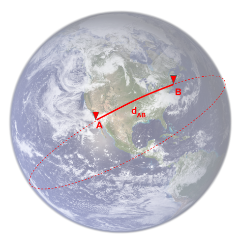
The guess function ignores the exact shape of the network but is able to say that, to go from A to B, you are more likely to find the shortest path by starting to move toward the right than toward the left, so you will arrive at the destination nodes in fewer iterations.
Using the haversine formula means that the A* algorithm with Neo4j can only be used if the nodes in the projected graph have spatial attributes (latitude and longitude).
Using A* within the Neo4j GDS plugin
The A* algorithm is accessible through the gds.alpha.shortestPath.astar procedure. The signature follows the same pattern as the other algorithms: the first parameter is the name of the projected graph the algorithm will use, while the second parameter is a map specific to each algorithm. In the A* algorithm configuration, we will find the same startNode, endNode, and relationshipWeightProperty we have already used for the shortestPath procedure. On top of that, two new properties are added to specify the name of the node property holding the latitude and longitude: propertyKeyLat and propertyKeyLon. Here is an example call to the A* algorithm on a projected graph:
MATCH (A:Node {name: "A"})
MATCH (B:Node {name: "B"})
CALL gds.alpha.shortestPath.astar.stream("graph", {
        startNode: A,
        endNode: B,
        relationshipWeightProperty: "weight",
        propertyKeyLat: "latitude",
        propertyKeyLon: "longitude",
    }
) YIELD nodeId, cost
RETURN gds.asNode(nodeId).name, cost
We will use this algorithm in the next chapter (Chapter 5, Spatial Data), where we will be able to build a real routing engine.
But before that, we will learn about other algorithms related to shortest pathfinding, such as the all-pairs shortest path or the spanning trees algorithms.
Discovering the other path-related algorithms in the GDS plugin
Being able to find the shortest path between two nodes is useful, but not always sufficient. Fortunately, shortest path algorithms can be extended to extract even more information about paths in a graph. The following subsections detail the parts of those algorithms that are implemented in the GDS plugin.
K-shortest path
Dijkstra's algorithm and the A* algorithm only return one possible shortest path between two nodes. If you are interested in the second shortest path, you will have to go for the k-shortest path or Yen's algorithm. Its usage within the GDS plugin is very similar to the previous algorithms we studied, except we have to specify the number of paths to return. In the following example, we specify k=2:
MATCH (A:Node {name: "A"})
MATCH (E:Node {name: "E"})
CALL gds.alpha.kShortestPaths.stream("graph_weighted", {
            startNode: A,
            endNode: E,
            k:2,
            relationshipWeightProperty: "weight"}
)
YIELD index, sourceNodeId, targetNodeId, nodeIds
RETURN index,
       gds.util.asNode(sourceNodeId).name as source,
       gds.util.asNode(targetNodeId).name as target,
       gds.util.asNodes(nodeIds) as path
The results are represented in the following table. The first shortest path is the one we already know: A, B, C, E. The second shortest path is A, C, E:
╒═══════╤════════╤════════╤═══════════════════════════════════════════════════════╕
│"index"│"source"│"target"│"path"                                                 │
╞═══════╪════════╪════════╪═══════════════════════════════════════════════════════╡
│0      │"A"     │"E"     │[{"name":"A"},{"name":"B"},{"name":"C"},{"name":"E"}]  │
├───────┼────────┼────────┼───────────────────────────────────────────────────────┤
│1      │"A"     │"E"     │[{"name":"A"},{"name":"C"},{"name":"E"}]               │
└───────┴────────┴────────┴───────────────────────────────────────────────────────┘
This algorithm can be very helpful when trying to define alternative routes.
Single Source Shortest Path (SSSP)
The aim of the SSSP algorithm is to find the shortest path between a given node and all other nodes in the graph. It is also based on Dijkstra's algorithm, but enables parallel execution by packaging nodes into buckets and processing each bucket individually. Parallelism is governed by the bucket size, itself determined by the delta parameter. When setting delta=1, SSSP is exactly equivalent to using Dijkstra's algorithm, meaning no parallelism is used. A value of delta that is too high (greater than the sum of all edge weights) would place all nodes in the same bucket, hence canceling the effect of parallelism.
The procedure in the GDS library is called deltaStepping. Its signature is as expected:
CALL gds.shortestPath.deltaStepping.stream(graphName::STRING, configuration::MAP)
Its configuration, however, is slightly different:
- startNode: The node from which all shortest paths will be computed
- relationshipWeightProperty: The usual relationship property carrying the weight
- delta: The delta parameter controlling the parallelism
With our simple graph, we can use this procedure with delta=1 using this query:
MATCH (A:Node {name: "A"})
CALL gds.alpha.shortestPath.deltaStepping.stream("graph_weighted", {
        startNode: A,
        relationshipWeightProperty: "weight",
        delta: 1
    }
)
YIELD nodeId, distance
RETURN gds.util.asNode(nodeId).name, distance
The returned values are as follows:
╒════════════════════════════╤══════════╕
│"gds.util.asNode(nodeId).name"│"distance"│
╞════════════════════════════╪══════════╡
│"A"                         │0.0       │
├────────────────────────────┼──────────┤
│"B"                         │10.0      │
├────────────────────────────┼──────────┤
│"C"                         │30.0      │
├────────────────────────────┼──────────┤
│"D"                         │35.0      │
├────────────────────────────┼──────────┤
│"E"                         │36.0      │
└────────────────────────────┴──────────┘
The first column contains each node in the graph, and the second column is the distance from the startNode, A, to each other node. We again encounter here the shortest distance from A to E of 36. We also find the results we found before when running Dijkstra's algorithm: the shortest distance between A and B is 10, and between A and C it's 30. On top of that, we have a new result: the shortest distance from A to D, which is 35.
All-pairs shortest path
The all-pairs shortest path algorithm goes even further: it returns the shortest path between each pair of nodes in the projected graph. It is equivalent to calling the SSSP for each node, but with performance optimizations to make it faster.
The GDS implementation procedure for this algorithm looks as follows:
CALL gds.alpha.allShortestPaths.stream(graphName::STRING, configuration::MAP)
YIELD sourceNodeId, targetNodeId, distance
The configuration parameters include, as usual, relationshipWeightProperty, the relationship property in the projected graph to be used as the weight.
There are two additional parameters to set the number of concurrent threads: concurrency and readConcurrency.
We can use it on our small test graph with the following:
CALL gds.alpha.allShortestPaths.stream("graph_weighted", {
 relationshipWeightProperty: "weight"
})
YIELD sourceNodeId, targetNodeId, distance
RETURN gds.util.asNode(sourceNodeId).name as start,
 gds.util.asNode(targetNodeId).name as end,
 distance
The result is the following matrix:
╒═══════╤═════╤══════════╕
│"start"│"end"│"distance"│
╞═══════╪═════╪══════════╡
│"B"    │"B"  │0.0       │
├───────┼─────┼──────────┤
│"B"    │"C"  │20.0      │
├───────┼─────┼──────────┤
│"B"    │"D"  │48.0      │
├───────┼─────┼──────────┤
│"B"    │"E"  │26.0      │
├───────┼─────┼──────────┤
│"A"    │"A"  │0.0       │
├───────┼─────┼──────────┤
│"A"    │"B"  │10.0      │
├───────┼─────┼──────────┤
│"A"    │"C"  │30.0      │
├───────┼─────┼──────────┤
│"A"    │"D"  │35.0      │
├───────┼─────┼──────────┤
│"A"    │"E"  │36.0      │
├───────┼─────┼──────────┤
│"C"    │"C"  │0.0       │
├───────┼─────┼──────────┤
│"C"    │"D"  │28.0      │
├───────┼─────┼──────────┤
│"C"    │"E"  │6.0       │
├───────┼─────┼──────────┤
│"D"    │"D"  │0.0       │
├───────┼─────┼──────────┤
│"D"    │"E"  │40.0      │
├───────┼─────┼──────────┤
│"E"    │"E"  │0.0       │
└───────┴─────┴──────────┘
You are now able to extract the following path-related information from your graph:
- One or several shortest paths between two nodes
- The shortest path between a node and all other nodes in the graph
- The shortest path between all pairs of nodes.
In the next section, we will talk about graph optimization problems. The traveling-salesman problem is the most famous graph optimization problem.
Optimizing processes using graphs
An optimization problem's objective is to find an optimal solution among a large set of candidates. The shape of your favorite soda can was derived from an optimization problem, trying to minimize the amount of material to use (the surface) for a given volume (33 cl). In this case, the surface, the quantity to minimize, is also called the objective function.
Optimization problems often come with some constraints on the variables. The fact that a length has to be positive is already a constraint, mathematically speaking. But constraints can be expressed in many different forms.
The simpler form of an optimization problem is so-called linear optimization, where both the objective function and the constraints are linear.
Graph optimization problems are also part of mathematical optimization problems. The most famous of them is the traveling-salesman problem (TSP). We are going to talk a bit more about this particular problem in the following section.
The traveling-salesman problem
The TSP is a famous problem in computer science. Given a list of cities and the shortest distance between each of them, the goal is to find the shortest path visiting all cities once and only once, and returning to the starting point. The following map illustrates a solution to the traveling-salesman problem, visiting some cities in Germany:

So we have an optimization problem with the following:
- An objective function: The cost of the path. This cost can be the total distance, but if the driver is only paid hourly, it may be more useful to use the total travel time as the objective to minimize.
- Constraints:
- Each city must be visited once and only once.
- The path must start and end in the same city.
Despite the straightforward formulation, this is an NP-hard problem. The only way to reach the exact solution in all cases is the brute-force approach, where you compute the shortest path between each pair of nodes (an application of the allPairsShortestPath algorithm) and checks all possible permutations. The time complexity of this approach is O(number of nodes!). You can imagine that with only a few nodes, this solution becomes impossible for a normal computer. Assuming each combination requires 1 ms processing time, a configuration with 15 nodes would require 15 ms, which would mean more than 41 years to test all possible combinations. With 20 nodes, this computation time increases to more than 77 million years.
Fortunately, some algorithms exist to find solutions that are not guaranteed to be 100% accurate, but close enough. Giving an exhaustive list of such solutions is out of the scope of this book, but we can quote two of the most common ones, both based on a science and nature analogy:
- Ant colony optimization (ACO): This algorithm is based on the observation of how ants communicate with each other in an ant colony using pheromones (odorous molecules) to achieve perfect synchronization. In the algorithm, many explorer ants (agents) are sent into the graph and travel along its edges based on some local optimization.
- Gene algorithms (GA): These are based on an analogy with genetics and how genes are propagated through generations via mutations in order to select the stronger individuals.
The TSP can be extended to even more complex use cases. For example, if a delivery company has more than one available vehicle, we can extend the TSP problem to determine the best course of action for more than one salesman. This is known as the multiple traveling-salesman problem (MTSP). More constraints can also be added, for instance:
- Capacity constraints, where each vehicle has a capacity constraint and can only carry up to a certain volume of goods.
- Time window constraints: In some cases, the package can only be delivered during a certain time window.
These TSP algorithms are not (yet) implemented in the GDS plugin. However, we can find an upper bound for the optimal solution using the spanning tree algorithm.
Spanning trees
A spanning tree is built from the original graph such that:
- The nodes in the spanning tree are the same as in the original graph.
- The spanning tree edges are chosen in the original graph such that all nodes in the spanning tree are connected, without creating loops.
The next figure illustrates some spanning trees for the graph we have studied in this chapter:

Among all possible spanning trees, the minimal spanning tree is the spanning tree with the lowest sum of weight for all edges. In the preceding diagram, the bottom-left spanning tree has a total sum of weights of 89 (10+33+6+40), while the bottom-right spanning tree has a total sum of weights of 64 (10+20+28+6). The bottom-right spanning tree is hence more likely to be the minimal spanning tree. To verify this, in the following section, we will discuss the algorithm implemented in the GDS plugin to find spanning trees, Prim's algorithm.
Prim's algorithm
This is how Prim's algorithm runs on our simple test graph:
- It chooses a starting node – node A in the following diagram.
- Iteration 1: It checks all edges connected to that node, and chooses the one with the lowest weight. Vertex B is selected and the edge between A and B is added to the tree.
- Starting from B, it visits C. Among C and D are already visited nodes. The one with the lowest weight is C, so C is selected and the edge between B and C is added to the tree.
- Starting from C, it can go to A, D, and E. A was already visited and the new edge (C->A) would add a higher weight than the already existing one, so this edge is skipped. However, you can see that the new edge reaching D (C->D) has a lower weight than the previously selected edge (A->D), meaning the previous edge is dropped from the tree and the new one is added.
- The last step consists of checking the last node, E. Here, adding the edge between D and E would increase the total weight by 40 instead of 6 (the weight of the edge between C and E), so this last edge is skipped.
The following diagram summarizes these four iterations, with edge creation (green lines), edges not taken into account (dashed green lines), and edges removed (dashed red lines):

The minimum spanning tree of our graph is then composed of the following edges:
A-B (weight 10)
B-C (weight 20)
C-D (weight 28)
C-E (weight 6)
You can check that all nodes are connected (there is a path between each pair of nodes in the graph) and the total weight is 64.
Let's try and retrieve this information from Neo4j.
Finding the minimum spanning tree in a Neo4j graph
The procedure to find the minimum spanning tree in the GDS plugin is as follows:
MATCH (A:Node {name: "A"})
CALL gds.alpha.spanningTree.minimum.write("graph_weighted", {
    startNodeId: id(A),
    relationshipWeightProperty: 'weight',
    writeProperty: 'MINST',
    weightWriteProperty: 'writeCost'
})
YIELD createMillis, computeMillis, writeMillis, effectiveNodeCount
RETURN *
This will actually create new relationships for each edge in the minimum spanning tree. To retrieve these edges, you can use the following:
MATCH (n)-[r:MST]-(m)
RETURN n, r, m
This query produces the following output, consistent with the result we obtained earlier by running Prim's algorithm:

Summary
This chapter was a long one, as it was our introduction to the GDS plugin. It is important to understand how to define the projected graph and the different entities to be included in it. We will see more examples in the following chapters, as we are going to use this library in all remaining chapters of the book.
The following table summarizes the different algorithms we have studied in this chapter, with some important characteristics to keep in mind:
| Algorithm | Description | Stream/Write | Negative weights |
| shortestPath | The shortest path between two nodes using Dijkstra's algorithm | Both | No |
| shortestPath.astar | The shortest path between two nodes using the A* algorithm and great circle heuristics (requires nodes with latitude and longitude properties) | Stream | No |
| kShortestPath | The k-shortest paths between two nodes using Yen's algorithm | Both | Yes |
| shortestPath.deltaStepping | Single source shortest path: the shortest path between a node and all other nodes in the graph | Both | No |
| allShortestPaths | The shortest path between each pair of nodes in the graph | Stream | No |
| spanningTree.* | The minimum, maximum, or k-spanning tree within a graph | Write | Yes |
As you will discover in the following chapters, shortest paths can also be used to infer other metrics on a graph, such as node importance (Chapter 5, Node Importance). But before going into those algorithms, as we talked a lot in this chapter about routing and geographical data, the next chapter will be dedicated to geodata management within Neo4j, using built-in data types and another Neo4j plugin: neo4j-spatial.
Questions
In order to test your understanding, try to answer the following questions. The answers are provided in the Assessment part at the end of this book:
- The GDS plugin and projected graphs:
- Why does the GDS plugin use projected graphs?
- Where are these projected graphs stored?
- What are the differences between named and anonymous projected graphs?
- Create a projected graph containing:
- Nodes: label Node
- Relationships: types REL1 and REL2
- Create a projected graph with:
- Nodes: labels Node1 and Node2
- Relationships: type REL1 and properties prop1 and prop2
- How do you consume the results of a graph algorithm from the GDS plugin?
- Pathfinding:
- Which algorithms are based on Dijkstra's algorithm?
- What is the important restriction regarding an edge's weight for these algorithms?
- What information is needed to use the A* algorithm?
Further reading
- Applications of graph algorithms in video games: Graph Algorithms for AI in Games [Video], D. Jallov, Packt Publishing
- An example project with custom functions and procedures is available at https://github.com/stellasia/neoplus .It includes an implementation of Dijkstra's algorithm using the Neo4j Java API.
- A* and heuristics: http://theory.stanford.edu/~amitp/GameProgramming/Heuristics.html
- Routing optimization solver, including the traveling-salesman problem, provided by Google: https://developers.google.com/optimization/routin