
Chapter 4
Reservoir Characterization and Simulation
Simplicity is the ultimate sophistication.
Leonardo da Vinci
Reservoir characterization is the process whereby a model of a subsurface body of rock is defined, incorporating all the distinguishing features that are pertinent to the reservoir capacity to accumulate hydrocarbons. One of the critical roles in traditional reservoir management is reservoir characterization as it enables the upstream engineers to make sound decisions regarding the exploitation of both oil and gas stored in these assets. The models strive to explain through simulation the behavior of fluids as they flow through the reservoir under a variable set of natural circumstances. The ultimate goal is to establish a suite of optimal strategies to maximize the production of the black gold.
Across the exploration and production (E&P) value chain the scope of success in drilling, completion, and production strategies hinges on the quantifiable accuracy of the reservoir characterization. An ever-increasing number of Society of Petroleum Engineers technical papers (Figure 4.1) are positioning data-driven models, analytics, and the range of soft computing techniques (neural networks, fuzzy logic, and genetic algorithms) as demonstrable processes to enhance the reservoir models.

Figure 4.1 Accelerated Uptake of Soft Computing Technical Papers
EXPLORATION AND PRODUCTION VALUE PROPOSITIONS
Often well data are deficient in regular quantity, and seismic data exhibit poor resolution owing to fractured reservoirs, basalt intrusions, and salt domes. Easy oil is a thing of the past and we are led to explore in uncharted frontiers such as deepwater environments and the unconventional reservoirs that house tight gas and oil-bearing shales. During the exploration, development, and production phases of such resources it is apparent that business strategies become more problematic and that perhaps the traditional approach that entails a deterministic study necessitates a supplementary methodology. The E&P value chain (Figure 4.2) opens multiple opportunities to garner knowledge from the disparate datasets by advocating a data-driven suite of workflows based on advanced analytical models and by establishing more robust reservoir models. Thus it is vital to adopt a hybrid stance that marries interpretation and soft computing methodologies to address business problems such as quantifying the accuracy of reservoir models and enhancing production performance as well as maximizing location of both production and injector wells.

Figure 4.2 Exploration and Production Value Chains
The oil and gas industry devotes a great deal of resources and expenditures in the upstream E&P domain. When we think about the lifecycle of an asset such as a well or reservoir, there is a business decision that must take place during each phase. That decision must have commercial value. You could be entering a new play and doing exploration to generate prospects, striving to gain insight from seismic and to locate exploratory wells in increasingly complex reservoirs. You need to appraise the commercial quantities of hydrocarbons and mitigate risks while drilling delineation wells to determine type, shape, and size of reservoir and strategies for optimum development.
During the development stage, a drilling program with optimized completion strategies is enacted as additional wells are located for the production stage. Surface facilities are designed for efficient oil and gas exploitation. Do we have to consider water production? What cumulative liquid productions do we anticipate? These are some of the questions we need to answer as we design those surface facilities.
The production phase necessitates efficient exploitation of the hydrocarbons. We have to consider health, safety, and environment (HSE) commitments and maintenance schedules. Is the production of hydrocarbons maximized for each well? How reliable are short- and long-term forecasts?
Maintaining optimal field production necessitates business decisions that determine whether an asset is economically viable. How do we identify wells that are ideal candidates for artificial lift? When and how do we stimulate a candidate well?
We have to be aware of the three major challenges across the E&P value chain:
- Data integration and management
- Quantification of the uncertainty in a multivariate subsurface system
- Risk assessment
These three tenets have recently been addressed by focusing a tremendous amount of effort to uncover innovative methodologies that can remediate the issues inherent in the traditional deterministic model-building exercises. The E&P problems are evolving into complex and undeterminable constraints on effective asset discovery, exploitation, and performance. There is a growing need for efficient data integration across all upstream disciplines as we strive to turn raw data into actionable knowledge by quantifying uncertainty and assessing from a probabilistic perspective a set of strategies that mitigate risk.
Soft computing techniques that entail descriptive and predictive analysis and adoption of data-driven analytics to mine ever-increasing volumes of disparate data force us to move from reactive to proactive management of oil and gas assets. The degree of comprehension moves from raw data through information and insight to actionable knowledge.
The analytical methodology must always start with an exploratory data analysis (EDA) step that surfaces hidden trends and relationships in the multivariate complex system that is a hydrocarbon reservoir. Do not model raw data; determine a suite of hypotheses worth modeling through an exploration of your key asset: data.
Let us concentrate on the soft computing techniques at our disposal to understand how reservoir characterization can be enhanced as we strive to quantify the uncertainty in the rock properties. We must ultimately mitigate risks associated with the field engineering tactics and strategies that evolve from a compressed decision-making cycle. We can accelerate this process by data-driven methodologies that employ advanced analytics.
As a field matures over age with production performance declining owing to natural pressure changes in the reservoir, it behooves a reappraisal step that again studies the hydrocarbon lifecycle through a dynamic body that is the reservoir. Reservoir characterization calibrated by history matching offers a more substantial geologic model to underpin that reappraisal step.
Reservoir characterization of a brownfield that has been producing for decades necessitates the analysis of invariably very large datasets aggregated from well logs, production history, and core analysis results enhanced by high-resolution mapping of seismic attributes to reservoir properties. It is imperative to surface the more subtle relationships inherent in these datasets, to comprehend the structure of the data, and identify the correlations in a complex multivariate system.
To accurately quantify the uncertainty in subsurface variables it is necessary to appreciate the heterogeneity of a complex system such as a hydrocarbon reservoir. How best to achieve this goal? We need to move away from the singular traditional deterministic modeling of data that are invariably raw with little or no quality control. Between 50 and 70 percent of time attributed to a reservoir characterization study should be invested in an analytical methodology that starts with a suite of data management workflows. You then design an iterative process implementing a data exploration to surface hidden patterns and comprehend correlations, trends, and relationships among those variables, both operational and nonoperational, that bear the most statistical influence on an objective function.
EXPLORATORY DATA ANALYSIS
EDA encompasses an iterative approach and enhances the process toward consistent data integration, data aggregation, and data management. EDA is achieved by adopting a suite of visualization techniques from a univariate, bivariate, and multivariate perspective.
Let us enumerate some of the common visualization techniques and build a logical sequence that underpins the methodology for efficient reservoir characterization projects during the exploration, development, and production stages in the E&P value chain. It is important to stress the positive impact behind the EDA school of thought that is often forgotten or even precluded prior to any traditional spatial analysis such as kriging, simulation, and uncertainty quantification steps. Figure 4.3 reflects a flowchart that typically engages the EDA methodology.
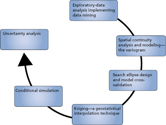
Figure 4.3 Reservoir Characterization Cycle
It is imperative to reduce the dimensionality of an engineering problem as complex systems invariably consist of a multivariate suite of independent and dependent variables. Which parameters are most sensitive statistically and hence most dominant or relevant vis-à-vis an objective function that can be identified as one or more dependent variables? We can address dimensionality and consequently formulate more realistic models by adopting a suite of analytical workflows that implement techniques such as principal component and factor analyses.
EDA1 is a philosophy for data analysis that employs a variety of techniques (mostly graphical) to achieve the following:
- Maximize insight into a dataset.
- Uncover underlying structure.
- Extract important variables.
- Detect outliers and anomalies.
- Test underlying assumptions.
- Develop parsimonious models.
- Determine optimal factor settings.
The main objective of any EDA study is to maximize insight into a dataset. Insight connotes ascertaining and disclosing underlying structure in the data. The significant and concrete insight for a dataset surfaces as the analyst aptly scrutinizes and explores the various nuances of the data. Any appreciation for the data is derived almost singularly from the use of various graphical techniques that yield the essence of the data. Thus, well-chosen graphics are not only irreplaceable, but also at the heart of all insightful determinations since there are no quantitative analogues adopted in a more classical approach. It is essential to draw upon your own pattern-recognition and correlative abilities while studying the graphical depictions of the data under study, and steer away from quantitative techniques that are classical in nature. However, EDA and classical schools of thought are not mutually exclusive and thus can complement each other during a reservoir characterization project.
In an EDA, workflow data collection is not followed by a model imposition; rather it is followed immediately by analysis and a goal of inferring what model would be appropriate. The focus is on the data, their structure, outliers, and models suggested by the data, and hence hypotheses that are worth pursuing. These techniques are generally graphical. They include scatterplots, character plots, box plots, histograms, probability plots, residual plots, and mean plots. EDA techniques do not share in the exactness or formality witnessed in the classical estimation techniques that tend to model the data prior to analysis. EDA techniques compensate for any paucity of rigor by adopting a very meaningful, characteristic, and insightful perspective about what the applicable model should be. There are two protocols that are imposed on the reservoir data and are model driven: deterministic modeling, such as regression models and analysis of variance (ANOVA) models, and probabilistic models that tend to assume that the errors inherent in deterministic models are normally distributed. Such a classical approach, quantitative in nature, is in contrast to the EDA methodology that does not impose deterministic or probabilistic models on the data, preferring the data to suggest acceptable models that reveal optimum fit to those data.
EDA techniques are thus instinctive and rely on interpretation that may vary across a broad scope of individual analysis, although experienced analysts invariably attain identical conclusions. Instead of adopting a classical filtering process that tends only to focus on a few important characteristics within a population by determining estimates, EDA exploits all available data to ensure that such inherent data characteristics such as skewness, kurtosis, and autocorrelation are not lost from that population. Also, unlike any intrinsic assumptions such as normality that are made in a classical approach, EDA techniques make few if any conjectures on upstream data, instead displaying all of the data. EDA strives to pursue as its goal any insight into the engineering or scientific process behind the data. Whereas summary statistics such as standard deviation and mean are passive and historical, EDA is active and futuristic. In order to comprehend the process and improve on it in the future, EDA implements the data as an aperture to delve into the core of the process that delivered the data.
Exploratory data analysis is used to identify systematic relationships between variables when there are no (or incomplete) a priori expectations as to the nature of those relationships. In a typical exploratory data analysis process, many variables are taken into account and compared, using a variety of techniques in the search for systematic patterns.
The basic statistical exploratory methods include examining distributions of variables (e.g., to identify highly skewed or non-normal, such as bimodal patterns), reviewing large correlation matrixes for coefficients that meet certain thresholds, or studying multi-way frequency tables (e.g., “slice-by-slice,” systematically reviewing combinations of levels of control variables). Multivariate exploratory techniques designed specifically to identify patterns in multivariate (or univariate, such as sequences of measurements) datasets include:
- Cluster analysis
- Factor analysis
- Discriminant function analysis
- Multidimensional scaling
- Log-linear analysis
- Canonical correlation
- Stepwise linear and nonlinear regression
- Correspondence analysis
- Time series analysis
- Classification trees
RESERVOIR CHARACTERIZATION CYCLE
It is essential to scrutinize the plethora of data across all upstream domains, integrating cleansed data from the geophysics, geology, and reservoir engineering fields. The effort afforded to this task is critical to the ultimate success of uncertainty analysis, and it is appropriate to adopt workflows to streamline the requisite EDA. Collating many different types of data across all geoscientific domains and applications can be contained in one analytical framework.
EDA itself can be partitioned into four discrete component steps:
- Step 1. Univariate analysis
- Step 2. Multivariate analysis
- Step 3. Data transformation
- Step 4. Discretization
The univariate analysis profiles the data and details traditional descriptors such as mean, median, mode, and standard deviation. Multivariate analysis examines relationships between two or more variables, implementing algorithms such as linear or multiple regression, correlation coefficient, cluster analysis, and discriminant analysis. The data transformation methodology encompasses the convenience of placing the data temporarily into a format applicable to particular types of analysis; for example, permeability is often transferred into logarithmic space to abide its relationship with porosity. Discretization embraces the process of coarsening or blocking data into layers consistent within a sequence-stratigraphic framework. Thus well-log data or core properties can be resampled into this space.
TRADITIONAL DATA ANALYSIS
EDA is a data analysis approach. What other data analysis approaches exist and how does EDA differ from these other approaches?
Three popular data analysis approaches are:
- Classical
- Exploratory (EDA)
- Bayesian
These three approaches are similar in that they all start with a general science and engineering problem and all yield science and engineering conclusions. The difference is in the sequence and focus of the intermediate steps.
For classical analysis the sequence is:

For EDA the sequence is:

For Bayesian the sequence is:

Thus for classical analysis, the data collection is followed by the imposition of a model (normality, linearity, etc.) and the analysis, estimation, and testing that follow are focused on the parameters of that model. For EDA, the data collection is not followed by a model imposition; rather it is followed immediately by analysis with a goal of inferring what model would be appropriate. Finally, for a Bayesian analysis, the analyst attempts to incorporate scientific and engineering knowledge and expertise into the analysis by imposing a data-independent distribution on the parameters of the selected model; the analysis thus consists of formally combining both the prior distribution on the parameters and the collected data to jointly make inferences and/or test assumptions about the model parameters.
The purpose of EDA is to generate hypotheses or clues that guide us in improving quality or process performance. Exploratory analysis is designed to find out “what the data are telling us.” Its basic intent is to search for interesting relationships and structures in a body of data and to exhibit the results in such a way as to make them recognizable. This process involves summarization, perhaps in the form of a few simple statistics (e.g., mean and variance of a set of data) or perhaps in the form of a simple plot (such as a scatterplot). It also involves exposure, that is, the presentation of the data so as to allow one to see both anticipated and unexpected characteristics of the data. Discover the unexpected prior to confirming the suspected in order to elucidate knowledge that leads to field development decisions.
In summary, it is important to remember the following tenets that underpin successful reservoir characterization from an EDA perspective:
- EDA is an iterative process that surfaces by trial-and-error insights and these intuitive observations garnered from each successive step are the platform for the subsequent steps.
- A model should be entertained at each EDA step, but not too much onus should be attributed to the model. Keep an open mind and flirt with skepticism regarding any potential relationships between the reservoir attributes.
- Look at the data from several perspectives. Do not preclude the EDA step in the reservoir characterization cycle if no immediate or apparent value appears to surface.
- EDA typically encompasses a suite of robust and resistant statistics and relies heavily on graphical techniques.
RESERVOIR SIMULATION MODELS
Habit is habit and not to be flung out of the window by any man, but coaxed downstairs a step at a time.
Mark Twain
A reservoir simulation is the traditional industry methodology to comprehend reservoir behavior with a view to forecasting future performance. On account of the complexities in the multivariate system that is the reservoir, a full-field simulation integrating both static and dynamic measurements yields a plausible model in the hands of expert engineers. However, this bottom-up approach starting with a geo-cellular model leading to a dynamic reservoir model is entrenched in first principles and fluid flow concepts that are solved numerically despite the inherent array of uncertainties and non-uniqueness in a calibration process such as history matching.
Top-down intelligent reservoir modeling (TDIRM), as postulated by Shahab Mohaghegh2 in several SPE papers and commentaries, offers an alternative methodology that strives to garner insight into the heterogeneous complexity by initiating workflows with actual field measurements. This approach is both complementary and efficient, especially in cost-prohibitive scenarios where traditional industry simulation demands immense time and resource investment to generate giant field simulations. In short, TDIRM and similar philosophical workflows implement AI and data mining techniques that are the themes threading this book together across the E&P value chain.
A rich array of advanced analytics provides efficient and simple approaches to flexible workflows to address exploratory data analysis, uncertainty analysis, and risk assessment in typical reservoir characterization projects. Adopting a visualization of analytics reduces the time to appreciate the underlying structure of the disparate upstream data that are prerequisites to making accurate reservoir management strategies.
Rich web-based solutions also enable efficient distribution to decision makers of the vital information and knowledge mined from the enormous amounts of data: well logs, core data, production data, seismic data, and well test data.
Analytical Simulation Workflow
Let us explore a logical suite of processes to enable more insight into reservoir simulation.
- Dividing fields into regions: Allowing for comparisons of well performance.
- Assisted and/or optimized history matching: Reducing uncertainty with reservoir characteristics.
- Identifying critical uncertainty factors: During the analysis of production data, screen data to identify and rank areas of potential production improvement.
- Analysis of history matching simulation runs: Targeting an understanding of how these several specific runs are different from each other (or what they have in common).
- Cluster analysis: Applying cluster analysis with segment profiling can give an additional insight into differences between history match simulation runs.
- Interactive data visualization: Visualization software allows very complex interactive visualizations owing to customization ability with proprietary scripting language that enhances analytic effectiveness for faster insights and actions.
- Benefits realization: The complex problem of the uncertainty assessment in performance forecasting is done with analytics using reservoir simulation models with extensive production history.
- Well correlations: Sophisticated data access and automated analyses of field data, such as well correlations, can now be processed in a significantly reduced amount of time.
- Decline curve analysis: Rather than blindly using all attributes of inputs for modeling, it is necessary to carry out an analysis to determine those attributes that bring a significant amount of useful information of the problem.
Let us explore the first three processes.
Dividing Fields into Regions
Leveraging nonlinear multivariate regressions, interpolation and smoothing procedures, principal component analysis, cluster analysis, and discrimination analysis, it is feasible to divide a field into discrete regions for field reengineering tactics and strategies. The methodology classifies the wells according to the production indicators, and divides the field into areas.
The statistical results can be mapped to identify the production mechanisms (e.g., best producers, depletion, pressure maintenance, and to identify and locate poorly drained zones potentially containing remaining reserves). Field reengineering can also be optimized by identifying those wells where the productivity can be improved.
The following list provides a short summary of the steps in wells classification process:
- Production statistics data preparation:
- Oil produced daily, water cut percent, gas produced daily.
- Decline curve analysis:
- Modeling daily production with nonlinear regressions.
- Data noise reduction and data interpolation:
- Implementation of smoothing methods that are most applicable to available data. For instance, in case of non-equally-spaced data you can use LOWESS (locally weighted least squares) smoothing methodology. Use resulting smoothed curves to interpolate missing data points for water cuts and GOR curves.
- Wells clustering:
- Principal component analysis:
- Used to create low-dimensional approximation to production dataset. This technique is often used before cluster analysis.
- Cluster analysis:
- Applied to condensed dataset with fewer factor scores (principal component analysis transformation of original variables).
- Analysis of clusters with different methods: segment profiling and dendrograms.
- Principal component analysis:
- Appraisal of wells representation:
- It can be useful for subsequent studies to have only a limited set of representative wells and to avoid intensive processing.
- Discriminant analysis:
- Performed to provide the probabilities of each well belonging to the obtained clusters.
Assisted and/or Optimized History Matching
The history matching process is conducted to reduce uncertainty regarding reservoir characteristics. This is done by matching simulation outputs with observed historical data (pressures, water cuts, etc.) by means of varying uncertainty matrix variables. Quality of the match is a statistical measure that identifies how close the simulation run matched the history (zero value would mean ideal match). It is beneficial to implement algorithms to semi-automate the process of searching for solution (Quality = 0) in a multidimensional space defined by the uncertainty matrix variables ranges. We define three main steps for this process:
- Step 1. Perform scoping runs: To explore relationships between uncertainty matrix variables and simulation outputs (response variables) and train initial estimates based on the information. Employ an Estimator, also called proxy or response surface model.
- Step 2. Perform most informative runs: Try to improve quality of the match by exploring solution space in the places that are the most promising according to currently available information in the Estimator.
- Step 3. Perform best match runs: Global optimization by all uncertainty matrix variables to fit Estimator (response surface model) to historical production data.
It is plausible to suppose that quality will converge to some value close to zero, which is not always true during a history matching process. By analyzing runs (using quality convergence, bracketing, and other types of runs analysis) we can determine if the simulations moved in the wrong direction and searched in the wrong place. In such a case the uncertainty matrix will be adjusted according to the reservoir characteristics knowledge already surfaced and the history matching process will be restarted from the beginning (scoping runs).
The main challenges in the process are:
- Identifying critical uncertainty factors: Which variables have the most impact on quality convergence?
- Analysis of simulation runs: Pattern discovery and comparison of simulation runs to reveal important differences.
- Adjusting uncertainty matrix: How to avoid human judgment errors.
Let us explore a functional history matching methodology that establishes a suite of models that fall above a level of quality imposed by reservoir engineers. Thus we tend to identify those models that have an objective function value under a predefined value. We are not then focused on optimization issues such as local minimum, convergence, and rapidity but more interested in how the quality of the model is measured. It is critical to define the objective function that measures the quality. Functional history matching is invariably coupled with uncertainty analysis that comes with an inflated price when addressed by traditional numerical simulations. We can demonstrate usage of simplified models known as proxies, touching on surface response models and artificial neural networks. The functional history matching approach is based on the work initiated by Reis, who proposes a process illustrated in Figure 4.4.
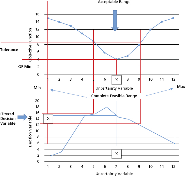
Figure 4.4 Filtering the Decision Variable
Let us assume that all input variables are known except one, so the objective function (OF) then depends on one single uncertainty variable. Considering the entire possible range of the values the uncertainty variable could represent, we would search for the minimum value of OF and then identify the “optimum” value x. In Figure 4.4 the value x correlates to the value y of the decision variable (e.g., NPV). However, this is the best model (uncertainty variable value) for the available information, but this model is not necessarily true. Instead of attaining the best model, a suite of models should be under investigation for subsequent analyses. This set of probabilistic models are within an acceptable range as constrained by the objective function and correspond to OF values above the minimum one in accordance to a tolerance threshold previously established by reservoir engineers.
Identifying Critical Uncertainty Factors
There are several tools that can help to resolve the problem of identifying critical factors from different perspectives:
- Decision tree analysis: automated or supervised learning.
- Variable importance based on statistical correlations and other measures.
- Regressions can additionally reveal interactions between uncertainty variables.
These techniques are applied to production data, well log data, and core data. Appreciating the stationarity assumptions along both the spatial plane and the temporal axis is important. During the analysis of production data it is necessary to screen the data to identify and rank areas of potential production improvement.
A decision tree represents a segmentation of the data that is created by applying a series of simple rules. Each rule assigns a simulation run to a segment based on the value of one input variable. One rule is applied after another, resulting in a hierarchy of segments within segments. The hierarchy is called a tree, and each segment is called a node. The original segment contains the entire dataset and is called the root node of the tree. Implementing such a technique identifies those reservoir properties that have most predictive power and hence most influence on a determinant or object variable such as OOIP or water cut.
An uncertainty matrix can have hundreds of potential variables that correspond to history match quality response (by means of simulator model). There are a number of statistical approaches to reduce the number of variables, which can be considered as determining variable importance in their power of predicting the match quality.
From a statistical standpoint this can be done by using R-square or Chi-square variable selection criterion (or their combination).
Surrogate Reservoir Models
Traditional proxy models such as the range of response surfaces or reduced models are piecemeal being replaced by surrogate reservoir models (SRMs) that are based on pattern recognition proficiencies inherent in an artificial intelligence and data mining school of thought. The numerical reservoir simulation model is a tutor to the SRM, training it to appreciate the physics and first principles of fluid flow through porous media of a specific reservoir as well as the heterogeneous and complex nature of the reservoir characteristics as depicted by the static geologic model. Fluid production and pressure gradients across the reservoir are instilled into the education of the SRM that is defined as a smart replica of a full-field reservoir simulation model.
SRMs offer a feasible alternative to the conventional geostatistical methodologies reflected by response surface and proxy models. As the objective function in uncertainty analysis, SRMs are effective in generating stochastic simulations of the reservoir, quantifying the uncertainty and thus mitigating some of the risks in performance prediction and field reengineering strategies. Additional benefits can be witnessed in real-time optimization and decision making based on real-time responses from the objective function.
Striving to resolve an inverse problem is a methodology that is a common denominator in building E&P models that have an ostensible analytical solution. The numerical solutions associated with traditional reservoir simulation practices are not ideal candidates to solve the inverse problem. SRMs provide the requisite tools to address the inverse problem in addition to furnishing a ranked suite of reservoir characteristics determined by key performance indicators that measure or quantify the influence or statistical impact each reservoir characteristic has on the simulation outcome, such as GOR or water cut.
CASE STUDIES
Predicting Reservoir Properties
Let us study a multivariate analytical methodology that incorporates a suite of soft computing workflows leading to a solution for the inverse problem of predicting reservoir properties across geologic layers in the absence of core data at localized wells.
One of the first steps is to implement a set of quantile–quantile (Q-Q) plots on the available data. The Q-Q plot is an exploratory graphical device used to check the validity of a distributional assumption for a dataset. The basic idea is to compute the theoretically expected value for each data point based on the distribution in question. If the data indeed follow the assumed distribution, then the points on the Q-Q plot will fall approximately on a straight line, as illustrated by the gamma ray variable in Figure 4.5.
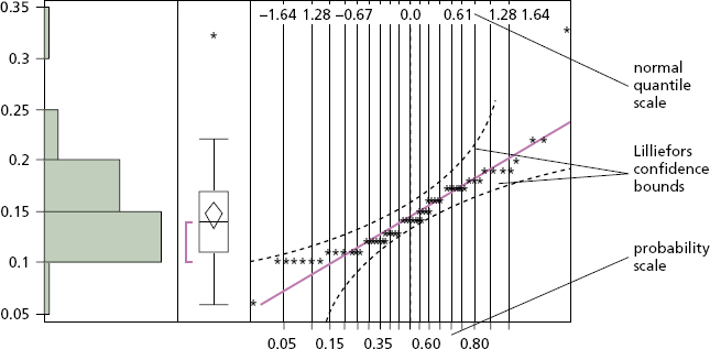
Figure 4.5 Gamma Ray Variable Displayed in a Q-Q Plot
The majority of the multivariate statistical techniques make the assumption that the data follow a multivariate normal distribution based on the experience that sampling distributions of multiple multivariate statistics are approximately normal in spite of the form of the parent population. This is due to the central-limit effect that in probability theory states that, given certain conditions, the mean of a sufficiently large number of independent random variables, each with a well-defined mean and well-defined variance, will be approximately normally distributed. The histogram and the cumulative distribution function (CDF) may be used to assess the assumption of normality by describing whether each variable follows a bell-shaped normal density (Figure 4.6).

Figure 4.6 Q-Q Plots with Histograms and CDFs for Three Gamma Ray Logs
Post Q-Q plots we can use principal components, factor analysis, and fuzzy logic concepts to identify the dominant variables and the optimum number of independent variables from the core and well logs that are available. It is imperative to reduce the dimensionality of the input space so as to reduce irrelevant variables that will cause the model to behave poorly. The neural network, for example, is somewhat undermined by addressing an input space of high dimensionality since we wish to avoid the neural network using almost all of its resources to represent irrelevant sections of the space.
In the subsurface the majority of reservoir characterization algorithms are nonlinear. Soft computing techniques have evolved exponentially during the recent decade to enable identification of nonlinear, temporal, and non-stationary systems such as hydrocarbon reservoirs.
If we are studying more than one regressor variable, it is plausible to scale the input data prior to creating the multiple regression model coefficients since scaling will ensure all input regressors will have equal variance and mean. Thus the subtle differences in the corresponding multiple regression coefficients will be indicative of the value ascertained for each regressor on the model. Let us consider, for example, the logarithmic value of permeability within a particular formation. Assume this logarithm is a function of porosity and gamma ray reading (lithology) that reflects a high and low influence on permeability, respectively.
What does this mean? It suggests that porosity has a more critical role to play in a multiple regression model than the gamma ray reading reflecting lithology differences. Let us define an algorithm (equation 1) that reflects an inoperative model:
There is no input or output scaling and the gamma ray in API units has more influence on the permeability owing to the scale of gamma ray and porosity, the latter being defined as a fraction.
Equation 2 may be positioned as a valid and logical model:
We now see both variables, gamma ray and porosity, at the same scale. Owing to the coefficient of porosity, it has a more critical influence upon the permeability. By scaling both the regressors and targets in the range [–1, 1] implementing equation 3 we are embracing the principle of equal variance and mean:
In equation 3, X represents any variable and reflects the importance of scaling to accurately model in a complex and multivariate system such as a hydrocarbon reservoir.
We can also reduce the dimensionality and reduce the effects of collinearity by adopting the technique of cross-correlation. The coefficients determined via cross-correlation are indicative of the extent and direction of correlation. By modeling any target variable that is representative of an objective function such as production rate or plateau duration, we can implement an analytical workflow that incorporates as input variables those that have a high correlation with the identified target or dependent variable.
If you want to see the arrangement of points across many correlated variables, you can use principal component analysis (PCA) to show the most prominent directions of the high-dimensional data. Using PCA reduces the dimensionality of a set of data and is a way to picture the structure of the data as completely as possible by using as few variables as possible.
For n original variables, n principal components are formed as follows:
- The first principal component is the linear combination of the standardized original variables that has the greatest possible variance.
- Each subsequent principal component is the linear combination of the variables that has the greatest possible variance and is uncorrelated with all previously defined components.
Each principal component is calculated by taking a linear combination of an eigenvector of the correlation matrix (or covariance matrix) with a variable. The eigenvalues show the variance of each component and since the principal components are orthogonal to each other there is no redundancy.
Principal components representation is important in visualizing multivariate data by reducing them to dimensionalities that are able to be graphed as the total variance represented by the original variables is equal to the total variance explicated by the principal components.
Once the input space has thus been reduced, we can implement a fuzzy logic process. Recall from Chapter 1 the logic behind fuzzy thinking and the historical commentary on Aristotle and Plato.
Aristotle formulated the Law of the Excluded Middle. It states that for any proposition, either that proposition is true, or its negation is true. The principle was stated as a theorem of propositional logic by Russell and Whitehead in Principia Mathematica.3 There is no middle or anything between the two parts of a contradiction where one proposition must be true and the other must be false.
However, human thought processes suggest otherwise, where the real world moves away from the bivalent black-and-white into the area that is somewhat gray! Is that why we refer to human brains as gray matter? How do we explain the variation in a curve that reflects a function of mineral volume in a specific rock based on gamma ray readings? Fuzzy logic rescues us from the Aristotelian manacles of Boolean logic. Essentially the world of fuzzy logic embraces four constitutional components:
- Fuzzification of input/output variables
- Fuzzy if–then rules
- Weighting factors
- De-fuzzification
Fuzzy logic is ostensibly a human appendage of conventional Boolean logic. As members of homo sapiens sapiens we tend to think as modern members of the human race, not in zeros and ones but in partial truths: those values that hover inexorably between “completely true” and “completely wrong.”
Aristotle’s laws of logic are founded on “X or not X”; it is either true or false. Inevitably we judge and classify in accordance to this stricture. We have an innate desire to categorize everything as it ameliorates our conventional thinking to drop something into a black or a white box. Of course the advent of computers only managed to reinforce this Boolean logic as a binary system underpins their natural reasoning mechanism.
But think about the constraints imposed by the Boolean logic in our thinking as we strive to establish analytical methodologies to help resolve business issues in the upstream E&P value chain. The continuous evolution of the multivariant, dynamic, and complex reservoir, for example, can only be described in a coarse approximation. Thus we are bereft of the essential details required to comprehend the possible solutions to a nondeterministic system. Let us not dismiss the range of probabilities established under uncertainty and described by confidence limits as we assess answers to subsurface questions. Not only does truth exist fundamentally on a moving scale, it is also discerned to change piecemeal by uncertainties in measurements and interpretations. Ironically, E&P engineers must move from the world of black-and-white into the “shadows” where gray predominates. This is the mathematics of fuzzy logic.
The multitude of possibilities that characterize this gray terrain must be tamed by quantification of the grayness or fuzziness. Probabilistic theory is the branch of mathematics concerned with probability, the analysis of random phenomena. The central objects of probability theory are random variables, stochastic processes, and events: mathematical abstractions of nondeterministic events or measured quantities that may either be single occurrences or evolve over time in an apparently random fashion. A random event can be described as an individual toss of a coin or the roll of dice, and if repeated many times, the sequence of these random events will exhibit certain patterns that can be studied and predicted.
Fuzzification of Input–Output Variables
Adopting applicable fuzzy sets controlled by membership functions, we can determine each variable’s degree of affiliation.
In equation 4, the elements expressed by z are in the universal set Z, and the fuzzy set A in Z is defined as a set of ordered pairs. The μA(z) is the membership function of z in A and maps each element of Z to a membership value between 0 and 1.
The calculation of the volume of clay in a specific rock such as limestone, for example, can be depicted by a curve based on gamma ray readings to identify inter-bedding occurrences. Such a calculation can be explicated by fuzzy logic as the gamma ray values (z) in the clay-volume (Z) in equation 4 where the membership function maps each gamma ray reading to a membership value between 0 and 1.
Fuzzy If–Then Rules
The rules are essentially statements of expression to embrace the imprecision inherent in the human thinking process. Here is one example of such a statement:
If the gamma ray value is high, then the clay-volume is large.
Note the lingual articulation of gamma ray and clay-volume associated with high and large labels. Of course we could adopt multiple parts to the antecedent and apply fuzzy logic operators AND, OR, and NOT to describe minimum, maximum, and complementary membership values of a variable.
Weighting Factors
If a single rule is inadequate, then multiple rules can be adopted, one playing off another. The fuzzy set that is an output from each rule can be amalgamated with other output fuzzy sets into a single output fuzzy set. As to the relative contributions of each output fuzzy set into the combined fuzzy set, a suite of weighting factors can be assigned to dictate the blended fuzzy output set. Engineering expertise and experience are salient designs on the weighting factors to abide by the different situations in a fuzzy inference system.
De-fuzzification
The fuzzy set or aggregated fuzzy set is input to a de-fuzzification process that generates a succinct value.
The next step in the methodology is application of a neural network. The human brain consists of a multitude of connected neurons. Artificial neural networks are adaptive, parallel information processing systems that can develop associations, transformations, or mappings between objects or data. They are thus efficient and popular techniques for solving regression and classification issues in the upstream oil and gas industry. The basic elements of a neural network are the neurons and their connection strengths or weights. In a supervised learning scenario a set of known input–output data patterns are implemented to train the network. The learning algorithm takes an initial model with some prior connection weights (random numbers) and applies an updating algorithm to produce final weights via an iterative process. Artificial neural networks (Figure 4.7) are used to build a representative model of predicting reservoir properties. The data are used as input–output pairs to train the neural network. Well information, reservoir quality data, and related data are used as input and are coupled with another category, production data, as output. Since first principles to model such a complex process using the conventional mathematical modeling techniques are tenuous at best, neural networks can provide an explicit insight into the complexities witnessed in characterizing reservoir properties in a spatiotemporal dimension. Once a reasonably accurate and representative neuro-model of the reservoir processes has been completed for the formation under study, more analysis can be performed. These analyses may include the use of the model in order to answer many what-if questions that may arise.

Figure 4.7 Artificial Neural Network
Maximizing Recovery Factors
Reservoir characterization studies necessitate an objective function be defined that drives the appropriate datasets aggregation and ultimately underpins the analytical methodologies to achieve accurate models. It is a continued industry problem to accurately forecast reservoir performance and classify assets as proved, probable, or possible. The reserves are directly tied to the recovery factor. Let us examine a probabilistic approach to qualify and quantify those variables that have a major influence on the recovery factor. The current world average recovery factor from oil fields is 30 to 35 percent (versus 20 percent in 1980). This parameter ranges from a 10 percent average of extra heavy crude oils to a 50 percent average of the most advanced fields in the North Sea. Increasing the recovery factor boosts reserves even without the discovery of new fields. Increasing by only 1 percent the recovery rate can increase reserves by 35 billion to 55 billion barrels—about one or two years of world oil production. In order to increase the hydrocarbon recovery factor it is necessary to improve the knowledge of oil fields and to use advanced technologies to drill wells and to produce hydrocarbons.
Future earnings are based upon the barrels of recoverable oil and/or gas described as a fraction of the size of the reservoir, and this is referred to as the recovery factor. However, there is an inherent degree of uncertainty as regards recoverability and economic viability of any proven reserves. The financial position of any public company depends on the amount of reserves located, the rate at which the reserves are recovered, and the economic and engineering principles and strategies incorporated by the company to optimize efficient reservoir.
An advanced analytical suite of workflows was implemented using multiple linear regression techniques to develop equations to elevate the recovery of hydrocarbons in terms of applicable reservoir rock properties and reservoir fluid properties. However, the first step on the road to determining appropriate algorithms for attaining improved recovery factors is to run an exploratory data analysis that entails techniques that are both graphical and quantitative in nature.
Most EDA techniques are graphical in nature with a few quantitative techniques. Graphics or visualizations provide unparalleled power to entice the data to reveal their structural secrets and surface correlations and trends that point the engineer in the right direction.
The particular graphical techniques employed in this case study are often quite simple. A 3D scatterplot shown in Figure 4.8 reveals relationships or associations among three variables. Such relationships manifest themselves by any nonrandom structure in the plot. Scatterplots can provide answers to the following questions:
- Are variables X and Y and Z related?
- Are variables X and Y and Z linearly related?
- Are variables X and Y and Z nonlinearly related?
- Does the variation in Z change depending on X or on Y?
- Are there outliers?
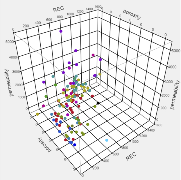
Figure 4.8 3D Scatterplot Surfacing Relationship among Porosity, Permeability, and the Objective Function Recovery Factor
To help visualize correlations, a scatterplot for each pair of response variables displays in a matrix arrangement, as shown in Figure 4.9. By default, a 95 percent bivariate normal density ellipse is imposed on each scatterplot. If the variables are bivariate normally distributed, this ellipse encloses approximately 95 percent of the points. The correlation of the variables is seen by the collapsing of the ellipse along the diagonal axis. If the ellipse is fairly round and is not diagonally oriented, the variables are uncorrelated.
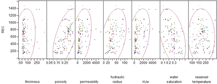
Figure 4.9 Scatterplot Matrix Illustrating Degrees of Correlation with the Recovery Factor
Thus it can be noted that the recovery factor has a strong correlation with the original oil in place (OOIP)—note the narrow and angled ellipse, a weaker correlation with porosity, permeability, and a lognormal distribution of water saturation—and even less correlation with the reservoir temperature, T.
With the wide spectrum of reservoir properties and the plethora of observations or rows of data, to guard against including any variables that have little contribution to the predictive power of a model in the population, a small significance level should be specified. In most applications many variables considered have some predictive power, however small. In order to choose a model that provides the best prediction using the sample estimates, we must guard against estimating more parameters than can be reliably estimated with the given sample size.
Consequently, a moderate significance level, perhaps in the range of 10 to 25 percent, may be appropriate, and the importance of thorough exploratory data analysis is underlined.
In Figure 4.10 a correlations table is depicted, which is a matrix of correlation coefficients that summarizes the strength of the linear relationships between each pair of response (Y) variables. This correlation matrix only uses the observations that have non-missing values for all variables in the analysis. It can be seen readily that the recovery factor has strongest correlations with both OOIP and porosity with Pearson correlation values of 0.7509 and 0.6089, respectively.
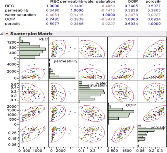
Figure 4.10 Multivariate Correlations of Influencing Reservoir Parameters
The multivariate simple statistics (mean, standard deviation, minimum, and maximum) provide a template for focused attention when considering the structure of data. These statistics can be calculated in two ways that differ when there are missing values in the data table. Multivariate simple statistics are calculated by dropping any row that has a missing value for any column in the analysis. These are the statistics that are used by the multivariate platform to calculate correlations. Generating a color map on correlations as in Figure 4.11 produces the cell plot showing the correlations among variables on a scale from red (+1) to blue (–1).
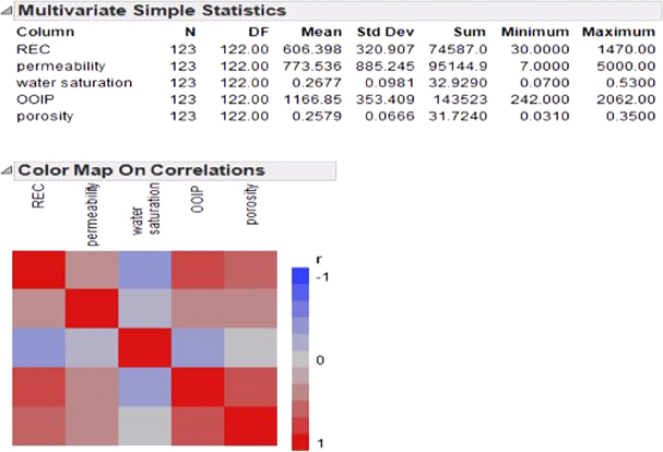
Figure 4.11 Color Map Depicting Correlations and the Analysis from a PCA
PCA is a technique to take linear combinations of the original variables such that the first principal component has maximum variation, the second principal component has the next most variation subject to being orthogonal to the first, and so on. PCA is implemented across a broad spectrum of geoscientific exploratory data in reservoir characterization projects. It is a technique for examining relationships among several quantitative variables. PCA can be used to summarize data and detect linear relationships. It can also be used for exploring polynomial relationships and for multivariate outlier detection. PCA reduces the dimensionality of a set of data while trying to preserve the structure, and thus can be used to reduce the number of variables in statistical analyses. The purpose of principal component analysis is to derive a small number of independent linear combinations (principal components) of a set of variables that retain as much of the information in the original variables as possible.
The PCA study calculates eigenvalues and eigenvectors from the uncorrected covariance matrix, corrected covariance matrix, or correlation matrix of input variables. Principal components are calculated from the eigenvectors and can be used as inputs for successor modeling nodes in a process flow. Since interpreting principal components is often problematic or impossible, it is much safer to view them simply as a mathematical transformation of the set of original variables.
A principal components analysis is useful for data interpretation and data dimension reduction. It is usually an intermediate step in the data mining process. Principal components are uncorrelated linear combinations of the original input variables; they depend on the covariance matrix or the correlation matrix of the original input variables. Principal components are usually treated as the new set of input variables for successor modeling nodes.
In PCA a set of dummy variables is created for each class of the categorical variables. Instead of original class variables, the dummy variables are used as interval input variables in the principal components analysis. The Ellipsoid 3D Plot toggles a 95 percent confidence ellipsoid around three chosen variables. When the command is first invoked, a dialog asks which three variables to include in the plot. The Pairwise Correlations table lists the Pearson product-moment correlations for each pair of Y variables, using all available values. The count values differ if any pair has a missing value for either variable. These are values produced by the Density Ellipse option on the Fit Y by X platform. The Pairwise Correlations report also shows significance probabilities and compares the correlations with a bar chart, as shown in Figure 4.12.
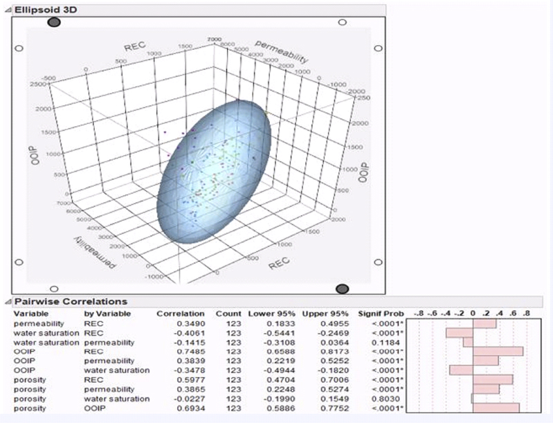
Figure 4.12 Pairwise Correlations Report with a 3D Scatterplot
Using a jackknife technique the distance for each observation is calculated with estimates of the mean, standard deviation, and correlation matrix that do not include the observation itself. The jackknifed distances are useful when there is an outlier as depicted in Figure 4.13. The plot includes the value of the calculated T2 statistic, as well as its upper control limit (UCL). Values that fall outside this limit may be an outlier.

Figure 4.13 Outlier Analysis with Upper Control Limit (UCL) Defined
Figure 4.14 illustrates three possible distributions for porosity: normal, lognormal, and Weibull. The normal fitting option estimates the parameters of the normal distribution based on the analysis sample. The parameters for the normal distribution are μ (mean), which defines the location of the distribution on the X-axis, and σ (standard deviation), which defines the dispersion or spread of the distribution. The standard normal distribution occurs when μ = 0 and σ = 1. The Parameter Estimates table for the normal distribution fit shows mu (estimate of μ) and sigma (estimate of σ), with upper and lower 95 percent confidence limits.
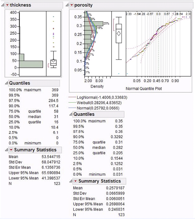
Figure 4.14 Distributions of Thickness and Porosity that Exhibit Predictive Powers for the Recovery Factor
Figure 4.14 also shows an overlay of the density curve on the histogram for porosity using the parameter estimates from the data. The lognormal fitting estimates the parameters μ (scale) and σ (shape) for the two-parameter lognormal distribution for a variable Y where Y is lognormal if and only if X = ln(Y) is normal. The Weibull distribution has different shapes depending on the values of α (scale) and β (shape). It often provides a good model for estimating the length of life, especially for mechanical devices and in biology. The two-parameter Weibull is the same as the three-parameter Weibull with a threshold (θ) parameter of zero.
The Smooth Curve option fits a smooth curve to the continuous variable histogram using nonparametric density estimation. The smooth curve displays with a slider beneath the plot. One can use the slider to set the kernel standard deviation. The estimate is formed by summing the normal densities of the kernel standard deviation located at each data point.
By changing the kernel standard deviation you can control the amount of smoothing. Thus, the results depicted graphically in Figures 4.14 and 4.15 provide a feel for the distribution of each reservoir property and associated structure of the underlying population data that have to be modeled. It is a necessary step in order to identify an appropriate model for the reservoir.

Figure 4.15 Continuous Parameters with Fitted Estimates
The partition platform recursively partitions the reservoir data according to a relationship between the X and Y values, creating a tree of partitions. It finds a set of cuts or groupings of X values that best predict a Y value. It does this by exhaustively searching all possible cuts or groupings. These splits of the data are done recursively, forming a tree of decision rules until the desired fit is reached.
Variations of this technique go by many names and brand names: decision tree, CARTTM, CHAIDTM, C4.5, C5, and others. The technique is often taught as a data mining technique, because
- It is good for exploring relationships without having a good prior model.
- It handles large problems easily.
- The results are very interpretable.
Each step of a partition tree analysis depicted in Figure 4.16 tries to split the reservoir data into two parts: a part with high mean value of REC (recovery factor) and a part with low mean value. At the first step, the high mean value of REC is “all observations such that OOIP has the value greater than or equal to 1032.” The other observations make up a set with low mean values of REC. At the second step, each of the sets in the first step is further subdivided. The “low mean value” group is split into a group where porosity < 0.282 and a second group where porosity > 0.282. The “high mean value” group is split into a group where Sw < 0.28 and the complement of that group.
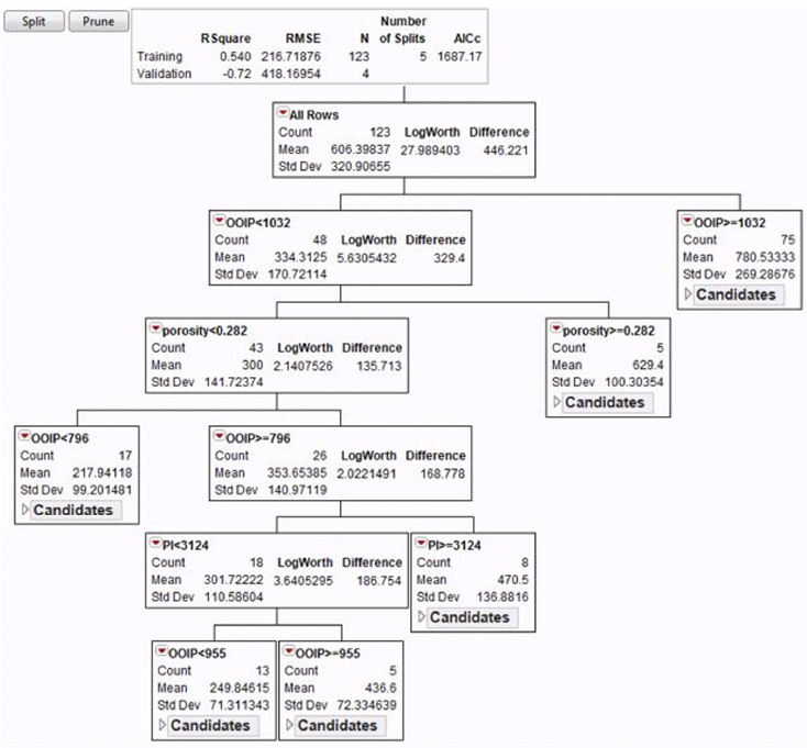
Figure 4.16 Partition Tree Classification
This process continues. The interpretation is a set of rules that predict high or low values of the REC variable or recovery factor. To find the largest values of REC, first choose observations where OOIP >= 1032. Within those, pick observations where Sw < 0.28. Continue for as many splits as one so desires. This partition tree model underlines the import of such parameters, OOIP and Sw, when determining an equation for the recovery factor of the reservoir.
Thus, it can be concluded from partition tree analysis that the most influential reservoir parameters and their associated values are: OOIP >= 1032, connate water saturation < 0.28, oil formation volume factor at abandonment pressure >= 1.234, and porosity > 0.256.
An empirical tree represents a segmentation of the data that is created by applying a series of simple rules. Each rule assigns an observation to a segment based on the value of one input. One rule is applied after another, resulting in a hierarchy of segments within segments. The hierarchy is called a tree, and each segment is called a node. The original segment contains the entire dataset and is called the root node of the tree. A node with all its successors forms a branch of the node that created it. The final nodes are called leaves. For each leaf, a decision is made and applied to all observations in the leaf. The type of decision depends on the context. In predictive modeling, the decision is simply the predicted value.
One can create decision trees that:
- Classify observations based on the values of nominal, binary, and ordinal targets.
- Predict outcomes for interval targets.
- Predict appropriate decisions when specifying decision alternatives.
An advantage of the decision tree is that it produces a model that may represent interpretable English rules or logic statements. Another advantage is the treatment of missing data. The search for a splitting rule uses the missing values of an input. Surrogate rules are available as backup when missing data prohibits the application of a splitting rule. Decision trees produce a set of rules that can be used to generate predictions for a new dataset. This information can then be used to drive business decisions.
If an observation contains a missing value, then by default that observation is not used for modeling by nodes such as neural network, or regression. However, rejecting all incomplete observations may ignore useful or important information that is still contained in the non-missing variables.
How can we deal with missing values? There is no single correct answer. Choosing the “best” missing value replacement technique inherently requires the researcher to make assumptions about the true (missing) data. For example, researchers often replace a missing value with the mean of the variable. This approach assumes that the variable’s data distribution follows a normal population response. Replacing missing values with the mean, median, or another measure of central tendency is simple, but it can greatly affect a variable’s sample distribution. You should use these replacement statistics carefully and only when the effect is minimal.
Another imputation technique replaces missing values with the mean of all other responses given by that data source. This assumes that the input from that specific data source conforms to a normal distribution. Another technique studies the data to see if the missing values occur in only a few variables. If those variables are determined to be insignificant, the variables can be rejected from the analysis. The observations can still be used by the modeling nodes.
Thus, exploratory data analysis should embrace a technique to identify missing data, so as to diligently handle such occurrences in light of the reservoir characterization project’s ultimate goal.