
Chapter 5
Drilling and Completion Optimization
Statistics are like a bikini. What they reveal is interesting. But what they hide is vital.
Aaron Levenstein
Drilling is one of the most critical, dangerous, complex, and costly operations in the oil and gas industry. While drilling costs represent nearly half of well expenditures, only 42 percent of the time is attributed to drilling. The remaining 58 percent is divided between drilling problems, rig movement, defects, and latency periods.
Some rigs are not fully automated and no single service company provides the full set of data operators need to comprehensively understand drilling performance. Unfortunately, errors made during the drilling process are very expensive. They occasionally damage reputation and result in hefty civil and government lawsuits and financial penalties (consider the 2010 BP Horizon deepwater fire and oil spill in the Gulf of Mexico). Inefficient drilling programs can have an even greater aggregate financial impact, causing delays in well completions or abandonments, unexpected shutdowns, hydrocarbon spills, and other accidents. There is a pressing need not only to improve drilling efficiency but also to predict hazardous situations that could have a negative impact on health, safety, and the environment.
Intelligent completions obtain downhole pressure and temperature data in real time to identify problems in the reservoir or wellbore and optimize production without costly well intervention. Sensing, data transmission, and remote control of zonal flow to isolate the formation from completion fluids help operators minimize fluid loss, manage the reservoir, maintain well integrity, and maximize production.
It is imperative for drilling personnel to understand the technical aspects of drilling and completion operations of a wellbore, to further enhance productivity of drilling and work-over projects, given the increasing demand for oil and natural gas.
The real-time drilling engineering process consists of four key stages to mitigate risks and preclude major issues, improve efficiency, and establish best practices, as depicted in Figure 5.1. It is paramount to integrate engineers’ experience and extant advanced technologies to generate business value within these stages:
- Stage 1. Alerts: Prevent operational problems from unexpected trend changes analyzing surface or downhole parameters.
- Stage 2. Judgments: Provide suggestions about hydraulic, torque and drag, and directional in order to improve the drilling performance of the well.
- Stage 3. Proposals: Propose significant changes on the well design, such as sidetrack, fishing options, unexpected high formation pressure analysis, total lost circulation, and casing point correlation.
- Stage 4. Methods: Adjust well program to improve the drilling performance.
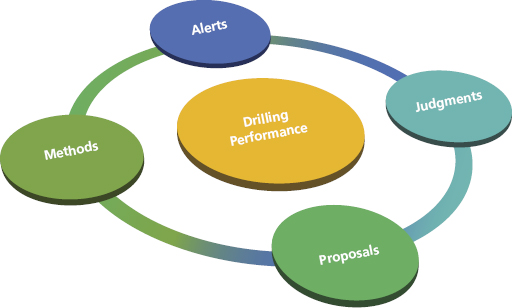
Figure 5.1 Real-Time Drilling Engineering Methodology
EXPLORATION AND PRODUCTION VALUE PROPOSITIONS
Drilling performance optimization is a knowledge-rich domain. It involves the application of drilling-related knowledge to identify and diagnose barriers to drilling performance and to implement procedural and/or technological changes to overcome these barriers. The overall objective of drilling performance optimization is that the well is drilled in the most efficient manner possible.
The knowledge required to execute drilling performance optimization is drawn from a multidisciplinary skillset within the drilling domain. Such skills include: fluids engineering, borehole pressure management, bottom-hole assembly (BHA) and drill-string design, drill bit selection, vibration management, and rock mechanics.
It necessitates a solution to provide a holistic view of the entire drilling system and gives near-real-time insight into parameters that can improve drilling efficiency, from planning through execution and completion.
- Uncover hidden patterns in data. Link data from nonoperational variables (rock properties, reservoir characteristics) with drilling operational parameters (weight on bit and revolutions per minute) and drilling system designs (drill bit models).
- Quantify drilling success. Data mining techniques applied to a comprehensive dataset identify potential correlations between drilling activity and incremental rate of penetration (ROP). This calculates drilling success in real time, under specific geomechanical conditions and constraints.
- Rely on root-cause analysis to guide decisions. Advanced analytical techniques gauge how to analyze real-time data relative to past performance or events so you can predict downhole tool failures and immediately determine which operational parameters to adjust.
- Improve drilling efficiency through its broad expertise in data integration, data quality, and advanced analytics, including optimization and data mining. Our solutions encourage collaboration and help operators make trustworthy, data-driven decisions.
- Identify key performance indicators (KPIs) behind efficient drilling operations. It is imperative to analyze the statistical relationship between data on relevant drilling incidents (e.g., equipment failures, well control issues, losses, stuck-pipes) and KPIs (e.g., ROP, cost per foot, and foot per day), given geomechanical constraints.
- Reduce nonproductive time with holistic data integration and management. Collects and analyzes key data from the entire drilling ecosystem, validates it with quality control processes, and then integrates it with an analytical data mart.
- Visualize and analyze drilling performance in near real time. Visualization offers quick-and-easy access to view the latest data on drilling parameters, events, and analytical results.
The system (Figure 5.2) combines multivariate, multidimensional, multivariant, and stochastic analytical workflows. Approaches using multivariate and/or multidimensional analysis fall short of representing a complex and heterogeneous system.

Figure 5.2 Multivariant, Multidimensional, Multivariate, and Stochastic Drilling
- Multivariant: Multiple independent variables that impact the outcome of a singularity.
- Multidimensional: Dimensions that affect the independent variables. For example, vibrations can be axial, tangential, and lateral.
- Multivariate: Multiple dependent variables that have to be predicted in order to reach an objective on a singularity. These are typically variables that have interdependencies that can affect the outcome of the singularity. For example, torque affects RPM, weight affects torque and RPM, and all three affect rate of penetration (the outcome).
- Stochastic: Variability and random behavior of independent variables. For example, the performance of the bit will vary depending on time, rock strength, flow rates, and so on.
WORKFLOW ONE: MITIGATION OF NONPRODUCTIVE TIME
The industry’s most common performance-quantifying metrics—cost per foot (CPF), foot per day (FPD), and rate of penetration (ROP)—are strongly influenced by mechanical specific energy (MSE), but MSE must not be equated to drilling efficiency alone. It is but one of several parameters that influence drilling productivity.
It is of paramount importance to analyze trends in all drilling performance-quantifying metrics to identify possible drilling inefficiencies, thereby learning from them and making adjustments to drilling parameters to attain an optimized drilling process. To achieve drilling efficiency, certain basic requirements and conditions must be met.
The ultimate objective must be geared toward confirming that the lowest cost per section and the construction of usable wells are the most critical factors in drilling performance and, if this is the case, defining the strategic initiatives and operational solutions that will lead there. In this regard, the sources of nonproductive time (NPT), namely visible lost time (VLT) and invisible lost time (ILT), must be analyzed in detail. Their contribution to the drilling performance has to be described analytically. Identification of other potential critical contributors to reduced drilling performance has to be performed analytically. Ultimately, the causes of these critical parameters along the drilling process need to be identified, and elimination of those primary inefficiency causes must be described as well.
To achieve this goal, drilling efficiency and ROP must both be defined, and factors influencing ROP and drilling efficiency must be identified. Most importantly, drilling efficiency’s different influencing factors, which include but are not limited to ROP, must be analyzed based on specific project objectives.
Drilling efficiency will have the desired effects on costs when all critical operational parameters are identified and assessed. These parameters, referred to as performance qualifiers (PQs), must be analyzed and quantified through an exploratory data analysis (EDA) methodology that surfaces hidden patterns and identifies trends and correlations in a multivariate complex system. Hypotheses worth modeling will be enumerated as a result of the EDA processes. The results will lead to a factual basis to allow governance over the drilling process, with performance evaluation logic established as business rules. Normalization and cleansing of key drilling parameters will provide a sound basis for EDA, leading to operational efficiency definition via business rules based on observations of scale and pattern variability.
To improve drilling efficiency, PQs should not be analyzed in isolation because they are interrelated. Consequently, maximization of any particular PQ, without identifying and addressing the effects the effort has on the other PQs, always compromises drilling efficiency.
The implementation of a Real-Time Operation Center (RTOC) addresses the increased complexity inherent in the volume and variety of drilling data currently collected from sensors in the wellbore as well as surface parameters, LWD, MWD, PWD, and third-party mud-logging data. Figure 5.3 illustrates some of the key stages in a real-time drilling engineering workflow that strives to attain best practices. The data management framework that encapsulates the information workflow and ensures the quality of the information generated in real time supports an effective decision-making cycle. Real-time information echoes the extant condition of the well under study. It is then a formality to integrate technical drilling applications into the process in real time.
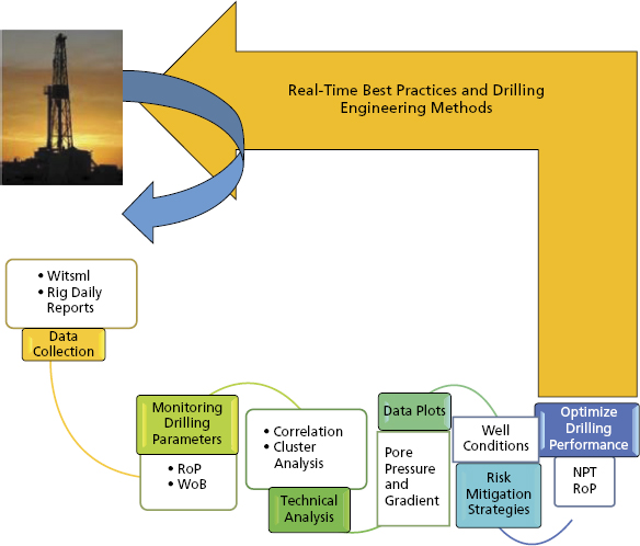
Figure 5.3 Real-Time Drilling Methodology
Advanced analytical workflows/processes can establish and evaluate key performance drivers that are fundamental to identification and reduction of nonproductive time (NPT) and invisible lost time (ILT) during drilling. By performing multivariate analysis on discrete data sources, analytical workflows can determine unknown patterns to identify trends in a drilling system. Through a suite of data cleansing, transformation, and exploratory data analysis (EDA) methodologies packaged in a new operational process for problem identification, selection, diagnosis, and solution finding, we will create models that define the correlations, trends, and signatures that predict stuck-pipe in an operationalized format that will enhance the drilling surveillance and control process.
There are multiple variables and components that comprise a drilling system, and therefore, many potential areas that may create challenges from an optimization perspective. By aggregating all of the relevant data (e.g., offset information, rock mechanics, mud properties, BHA design, rig capabilities, etc.) we are able to generate models that can predict potential points within the drilling system that could be optimized. Analytical workflows/processes can then be developed to achieve many goals, including:
- Continuous levels of improvement through the automation of the entire workflow
- Data validation to build accurate advanced analytical models
- Root-cause analysis to identify key performance indicators and their range of operational values covering different functions in the drilling process, including the following:
- Wellbore quality: Avoid potential issues such as stuck-pipe associated with borehole cleaning activities.
- Rig performance: Why specific rigs perform better than others in the same asset/play.
- Optimize drilling operations by gathering and analyzing both static and real-time drilling data.
- Wellbore stability: Establish a suite of methodologies to model and forecast borehole stability.
- Real-time identification of wellbore instability and associated modes of failure.
- Forecasting workflows that encapsulate drilling parameters to preclude unstable wellbore designs.
- Well pressure management: Methodologies to analyze and monitor various pressures.
In addition to a data-driven system that translates raw data into tangible and effective knowledge, we see the juxtaposition of a user-driven system underpinned by expert knowledge garnered through experience as completing a hybrid approach. This composition of different or incongruous data sources underpins a soft computing technique driven by a methodology based on advanced analytical workflows implementing self-organizing maps (SOMs), clustering, and Bayesian approaches. The data-driven approach necessitates a robust and quality-assured stream of data.
A solution architecture to realize and estimate events leading to NPT is illustrated in Figure 5.4. We must analyze the historical frequency and probability of occurrence, cross-matching faults with service companies and resources to enhance early decision making. It is necessary to establish a workflow to identify critical wells with higher probability of experiencing NPTs as candidates for remediation and rank a comparison of NPT events between wells.
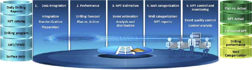
Figure 5.4 Solution Architecture to Reduce NPT
The NPT identification solution can iterate through several layers of integrated and logical workflows that form a top-down methodology (Figure 5.5) that ultimately morphs into a catalog of historical events with associated diagnoses and best practices for remediation.
Figure 5.5 NPT Catalog
Segment wells in accordance with the tactics/strategies and NPT events, as illustrated in Figure 5.6. Business objectives determine a well segmentation via a clustering module to characterize on a geographical basis. Relate NPTs to specific drilling companies and crews.

Figure 5.6 Cluster Analysis to Identify Similar Classes by Tactics/Strategies and NPT
Pareto charts help to identify the most important NPTs by well and/or field, considering their impact by length of time delays. They endorse the definition of priorities for quality improvement activities by identifying the problems that require the most attention. And control graphs by well and fault category enable the identification of critical faults and their impact in drilling depth and performance times as well as the recognition of out-of-control faults. Both forms of visualization underpin the NPT methodology depicted in Figure 5.7.
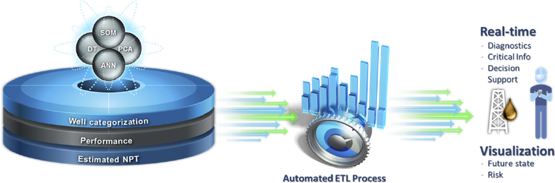
Figure 5.7 NPT Methodology
Let us develop a workflow based on a best practice methodology to reduce NPT by minimizing the occurrences of stuck-pipe events.
Stuck-Pipe Model
What is stuck-pipe, and what are the benefits to obviate the effects of such an occurrence? During the drilling operation the drill string sticks while drilling, making a connection, performing logging, or any operation that involves the equipment being left in the hole. Stuck-pipe issues invariably fall into two categories: mechanical and differential. The former occurs while the drill string is mobile and an obstruction or physical constraint results in the sticking event. Such conditions are realized in wellbore instability situations such as poor hole cleaning that triggers high torque, excessive drag on the drill string, and hole pack-off, leading to stuck-pipe. The latter occurs due to a higher pressure in the mud than in the formation fluid. Differential sticking is witnessed when the drill collar rests against the borehole wall, sinking into the mudcake. The area of the drill collar that is not embedded into the mudcake has a pressure acting upon it that is equal to the hydrostatic pressure (Ph) in the drilling mud, whereas that area embedded exhibits a pressure equal to the rock formation pressure (Pf) acting upon it. Figure 5.8 illustrates the hydrostatic pressure in the wellbore being higher than the formation pressure, resulting in a net force pushing the collar toward the borehole wall.
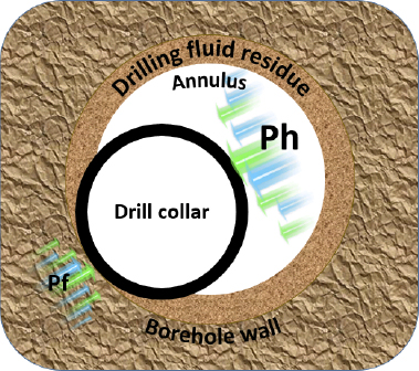
Figure 5.8 Differential Sticking: Ph (Hydrostatic Pressure) Exhibiting a Higher Value than Pf (Pore Pressure of a Permeable Formation)
Thus, a stuck-pipe incident is a pervasive technical challenge that invariably results in a significant amount of downtime and increase in remedial costs. The drilling of oil and gas wells is a process fraught with potential issues and the multiple mechanisms that can contribute to a stuck-pipe situation have to be discriminated in order to identify those operational and nonoperational parameters that have a major impact on each mechanism. To preclude the adverse impact of attaining critical success targets in a drilling program and in light of recent increases in drilling activity in high-risk assets compounded by an ever-increasing shortage of experienced drilling personnel, it is imperative to introduce an advanced analytical suite of methodologies that deploy a hybrid solution to address such drilling issues. Such a hybrid solution, delivered around a combined user-centric system based on experience and a data-driven component that captures historical data, enables engineers, both young and old, to gain crucial time-critical insights to those parameters that have a major statistical impact on a stuck-pipe incident.
Understanding and anticipating drilling problems, assessing their causes, and planning solutions are necessary for overall-well-cost control and for successfully reaching the target zone. Thus the benefits are both tangible and economically viable to identify methodologies, both deterministic and stochastic, that mitigate the risk and even predict the occurrence of the sticking event and ultimately ensure wellbore integrity that precludes wellbore instability (Figure 5.9) leading to stuck-pipe.
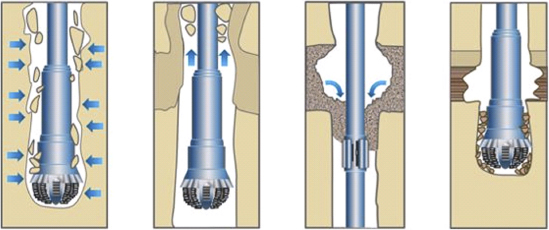
Figure 5.9 Wellbore Instability Is Prone to a Stuck-Pipe Event, Leading to NPT
There are multiple mechanisms that can contribute to a stuck-pipe situation. One of the major technical challenges of the drilling program is the frequency of stuck-pipe incidents. Such occurrences invariably result in a significant amount of downtime and increase in remedial costs, adversely impacting the attainment of the critical success targets of the drilling program. Unfortunately, with the recent increase in drilling activity and shortage of experienced drilling personnel, drilling in high-risk assets has augmented the potential of stuck-pipe events.
How do we identify the onset of stuck-pipe in all its forms, find the most critical and frequent stuck-pipe scenarios, diagnose them, and find an operational solution that prevents or mitigates their occurrence? In order to do this it is necessary to analyze and quantify the parameters most influential for all stuck-pipe mechanisms, segment scenarios by signature of behavior of groups of parameters, rank these scenarios by frequency and criticality, select the few top-ranking scenarios, perform causal analysis in order to detect early indicators, and at the same time issue a predictive model to be used operationally. At the end of this process, and under the assumption that the predictive indicators offer a lead time long enough for operators to act, a decision needs to be made on operational actions to be taken in order to prevent or significantly mitigate the analyzed scenario.
Thus, the long-term goal is to identify preventative or mitigating measures in light of warning signs hidden in the appropriate operational and nonoperational parameters deemed necessary for each stuck-pipe mechanism.
The principal data required are:
- Rock mechanics data
- Fluids data
- Lithological data
- BHA dynamics data
- Vibration data
- MWD/LWD data
- Surface equipment data
WORKFLOW TWO: DRILLING PARAMETER OPTIMIZATION
In order to attain minimum cost per foot with an understanding of uncertainty quantification and controlled risk assessment, a drill bit optimization methodology identifies the optimum drill bit for the drilled interval. Incorporate offset well data to select appropriate drill bit and associated critical characteristics. The advanced analytical workflows embrace a thorough analysis of offset well data, including well logs, formation tops, mud logs, core analysis, rock mechanics, drilling parameters, bit records, and dull bit conditions.
Adopting tailored analytical workflows that incorporate disparate datasets it is feasible to attain minimum cost per foot with an understanding of uncertainty quantification and controlled risk assessment in a drill bit optimization methodology. Such an evaluation process would include such steps as:
- Evaluation of expected formation types
- Offset well data gathering
- Determination of unconfined compressive rock strength, effective porosity, abrasion characteristics, and impact potential
- Identification of potentially optimal bit types and various applicable characteristics
- Prediction of cost per foot for each potential bit
- Optimal drill bit recommendation
Post-run, analysis evaluates bit performance from available data such as real-time ROP, RPM, torque, and drill bit conditions. Such analytical results offer design and application feedback to engineers for an iterative and continuous-improvement process.
Well Control
The methodology typically requires multiple iterations of analytical cycles to monitor the various pressures in real time: drilling fluid pressure in the well, gas, oil, and water under pressure (formation pressure), and mud pressure. If the formation pressure is greater than the mud pressure, there is the possibility of a blowout.
Drilling Optimization Analytical Project:
- An automated process to measure both actual and theoretical drill bit performance and detect abnormal deviations.
- Creation of a multivariate statistical model that automatically identifies and quantifies the drivers of drill bit performance.
- Daily reports facilitate event detection and alerting in drilling surveillance.
- Insight into the performance functions and their drivers one by one and in combination: This enables engineers in surveillance, reliability, process, and operations to understand the drivers’ significance in abnormal performance states, detect patterns of performance deviation and their indicators, find causes, improve the patterns with analytical cause indicators, determine short-term performance and long-term reliability risks, and develop prevention measures.
By aggregating all relevant data (such as offset information, rock mechanics, mud properties, BHA design, rig capabilities, etc.) we are able to generate models that can predict potential points within the drilling system that could be optimized. Analytical workflows/processes can be developed to achieve many goals, including:
- The validation of data to build accurate advanced analytic models.
- Continuous levels of improvement through the automation of the entire workflow.
- Root-cause analysis to identify key performance indicators and their range of operational values covering different functions in the drilling process, including the following:
- Wellbore integrity/quality: Avoid potential issues, such as stuck-pipe, associated with hole-cleaning activities.
- Rig performance or rig-state detection: Examine why specific rigs perform better than others in the same asset/play. Optimize drilling operations by gathering and analyzing both static and real-time drilling data during execution and post-drilling operations.
- Wellbore stability: Establish a suite of methodologies to model and forecast borehole stability. In real time, identify wellbore instability and associated modes of failure to minimize cost and optimize drilling regimes. Create a forecasting workflow that encapsulates and analyzes drilling parameters to preclude expensive and unstable wellbore designs.
- Well control: Methodology to analyze and monitor various pressures.
By taking a holistic view of the entire drilling system, analytic models are able to determine the key performance attributes within each discrete component and determine the correlation between multiple variables.
Real-Time Data Interpretation to Predict Future Events
Advanced analytical techniques can be applied to gauge how real-time data are analyzed relative to past performance/events to predict downhole tool failures and the ability to do immediate root-causal activities and implement real-time solutions.
Comparing real-time drilling data against previous trends allows for the following:
- Avoid potential NPT by predicting a failure, such as a PDM due to excessive vibration.
- Geo-steering: Able to make real-time adjustments to the wellbore trajectory (i.e., unforeseen transition zones).
- Able to make real-time drilling parameter changes (i.e., WOB, TOB, flow rate).
- Prevent blowouts: Multivariate iterative process to analyze pressures such as formation, mud, and drilling fluid pressures.
Statistical analysis uses predefined patterns (parametric model) and compares measures of observations to standard metrics of the model, testing hypotheses. We implement a model to characterize a pattern in the drilling data and match predetermined patterns to data deductively following the Aristotelian path to the truth. We then build a model with the drilling data and thus do not start with a model. Patterns in the data are used to build a model and discover patterns in the data inductively following a Platonic approach to the truth.
- Data management
- Data quality
- Predictive modeling and data mining
- Reporting of results
It is necessary to develop workflows for each of the above capabilities to preclude significant amounts of manual intervention and provide efficient and streamlined processes that are consistent and repeatable across multiple disparate global assets. As your drilling problems become too complex to rely on one discipline and as you find yourselves in the midst of an information explosion, multidisciplinary analysis methods and data mining approaches become more of a necessity than professional curiosity. To tackle difficult problems in drilling unconventional plays, you need to bring down the walls built around traditional disciplines and embark on true multidisciplinary solutions underpinned by advanced analytical workflows.
CASE STUDIES
Steam-Assisted Gravity Drainage Completion
With the production of bitumen and heavy oils becoming economically viable, Dr. Roger Butler’s SAGD1 (steam-assisted gravity drainage) technique has become an oilfield norm in such assets. As with all unconventional oil production, SAGD is a complex and dynamic operational process where subsurface influences are managed from a surface control location. This blend of mechanical systems and subsurface heterogeneity creates a stochastic system riddled with uncertainty. Attaining a reduction in the variable production costs and an increase in recovery rate necessitates a decrease in steam–oil ratio (SOR). In turn SOR is optimized by reducing the steam injection rates and/or increasing oil production.
The emergence of downhole distributed sensing (DTS) combined with the artificial lift and reservoir properties provides a rich multivariate dataset. In this case study we shall present a data-driven approach where observed behaviors from a SAGD operation are used to model a dynamic process constrained by first principles, such that we can leverage the large volumes and varieties of data collected to improve operational effectiveness of the SAGD process. Finally, let us demonstrate how an analytical model for SAGD can be placed into a closed loop system and used to automate heavy oil production in a predictable and predetermined manner, ensuring consistent and optimized completion strategies in such assets.
In the SAGD process, two parallel horizontal oil wells are drilled in the formation, one about four to six meters above the other. The upper well injects steam, and the lower one collects the heated crude oil or bitumen that flows out of the formation, along with any water from the condensation of injected steam. The basis of the process is that the injected steam forms a “steam chamber” that grows vertically and horizontally in the formation. The heat from the steam reduces the viscosity of the heavy crude oil or bitumen, which allows it to flow down into the lower wellbore. The steam and gases rise because of their low density compared to the heavy crude oil below, ensuring that steam is not produced at the lower production well. The gases released, which include methane, carbon dioxide, and usually some hydrogen sulfide, tend to rise in the steam chamber, filling the void space left by the oil and, to a certain extent, forming an insulating heat blanket above the steam. Oil and water flow is by a countercurrent, gravity-driven drainage into the lower wellbore. The condensed water and crude oil or bitumen is recovered to the surface by pumps such as progressive cavity pumps, which work well for moving high-viscosity fluids with suspended solids.
A key measure of efficiency for operations using SAGD technology is the amount of steam needed to produce a barrel of oil, called steam-to-oil ratio (SOR). A low SOR allows us to grow and sustain production with comparatively smaller plants and lower energy usage and emissions, all of which results in a smaller environmental footprint.
The data-driven methodology strives to ascertain the optimal values for those control variables that lead to maximum oil production:
- Pump speed
- Short injection string
- Long injection string
- Casing gas
- Header pressure
- Produced emulsion
There are three potential workflows that constitute a multivariate methodology:
- Workflow 1: Assumptions are made on the predetermined behavior on the data.
- Implement linear regression models.
- Dependent variables:
- Water
- Oil
- Independent variables:
- Production to header pressure
- Casing gas to header pressure
- Pump speed
- Injection steam to short tubing
- Injection steam to long tubing
- Dependent variables:
- Implement linear regression models.
- Workflow 2: No assumptions are made on any predetermined behavior on the data.
- Implement neural networks models.
- Output variables:
- Water
- Oil
- Input variables:
- Production to header pressure
- Casing gas to header pressure
- Pump speed
- Injection steam to short tubing
- Injection steam to long tubing
- Output variables:
- Workflow 3: Does not assume any predetermined behavior on the data and assumes no model formulation.
- Implement association rules.
- Surfaces IF/THEN-type rules in the data.
- Implement association rules.
- Implement neural networks models.
The analytical workflows aggregated data from two well pads with focus on two well pairs: P1 and P3. We separated the dependent variables, water and oil, from the production emulsion based on the water-cut values across the input domain. The input data did not include any nonoperational parameters such as reservoir properties or geomechanics. We set aside 75 percent of the extant data for training purposes to build the models; the remaining 25 percent was used for validation purposes.
Workflow One
The left-hand side of Figure 5.10 details the linear regression model for water production, whereas the right-hand side represents the results applied to oil production data. Note that oil was overpredicted and conversely water was underpredicted. The values of R-squared for water and oil are 0.7188 and 0.3411, respectively. The value R-squared is the coefficient of determination and reflects how well the data points fit the regression line.
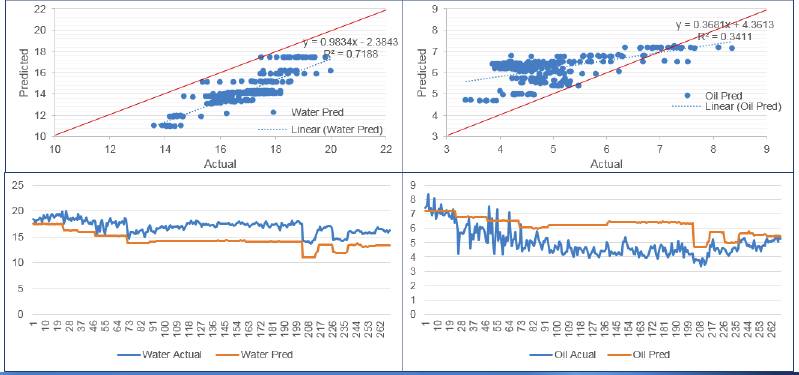
Figure 5.10 Study Results for Well Pair 1
Workflow Two
The neural network implemented was a feed-forward adaptation with a supervised learning mode with back-propagation to perform sensitivity analysis that determines how each input parameter influences the output (water and oil production; see Figure 5.11). Thus there were five input variables for each neural network modeling water and oil production. The hidden nodes were constrained to two or three.
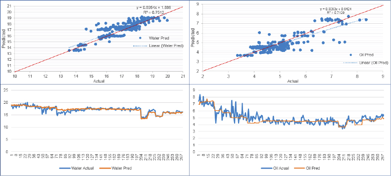
Figure 5.11 Neural Network Models for Water and Oil for Well Pair 3
The R-squared values for water and oil are comparable, each about 0.7, thus illustrating a pretty good correlation. It appears that the multivariate analysis workflow implementing the artificial neural network provides a very good methodology to predict the production of either water or oil.
Workflow Three
The final approach utilized five association rules as detailed in Figures 5.12 and 5.13 for well pairs 1 and 3, respectively.
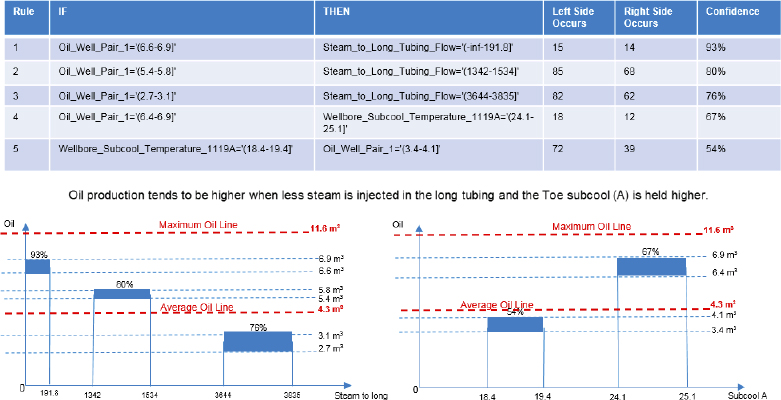
Figure 5.12 Association Rules Implemented on SAGD Dataset for Well Pair 1
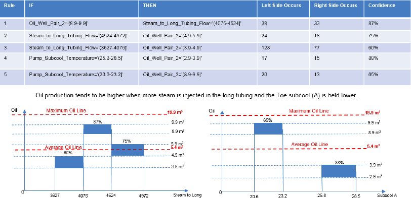
Figure 5.13 Association Rules Implemented on SAGD Dataset for Well Pair 3
Conclusions
Selecting optimal control variables for well pairs 1 and 3 we concluded that a three-step diagnosis was applicable:
- Step 1. Implement the estimated coefficients from workflow 1 or the weights ascertained in workflow 2.
- Step 2. Adopt the ranges suggested for the control variables by the association rules in workflow 3 and implement them as constraints for a nonlinear programming model.
- Step 3. Establish an objective function.
Perusing the outputs from the three workflows we derived the following functional relationships for each well pair that could subsequently be operationalized in a closed loop process to maximize hydrocarbon production via a suite of operational parameters controlled in the SAGD completion.
Well Pair 1:
- Objective Function: MAX Oil =
- 0.000117∗Well_Production_to_Header_Pressure
- − 0.000732∗Well_Casing_Gas_to_Header_Pressure +
- 0.0976∗Pump_Speed_Reference_in_Hertz
- − 0.000034∗Steam_to_Short_Tubing –
- 0.000299∗Steam_to_Long_Tubing
- Subject to (Figure 5.14):
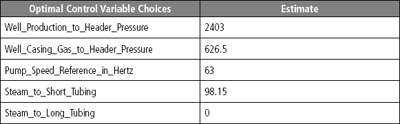
Figure 5.14 Optimal Control Variable Values for Well Pair 1
- Subject to (Figure 5.14):
- 2396 < Well_Production_to_Header_Pressure <= 2403
- 626.5 < Well_Casing_Gas_to_Header_Pressure <= 677.8
- 62.5 < Pump_Speed_Reference_in_Hertz <=63
- 98.15 < Steam_to_Short_Tubing <= 10516
- 0 < Steam_to_Long_Tubing <= 191.8
Well Pair 3:
- Objective Function: MAX Oil = –
- 0.003300∗Well_Production_to_Header_Pressure
- + 0.001091∗Well_Casing_Gas_to_Header_Pressure +
- 0.2674∗Pump_Speed_Reference_in_Hertz
- – 0.000226∗Steam_to_Short_Tubing +
- 0.0000133∗Steam_to_Long_Tubing
- Subject to (Figure 5.15):

Figure 5.15 Optimal Control Variable Values for Well Pair 3
- Subject to (Figure 5.15):
- 2289 < Well_Production_to_Header_Pressure <= 2307
- 1172 < Well_Casing_Gas_to_Header_Pressure <= 1211
- 64 <Pump_Speed_Reference_in_Hertz <= 65
- 10969 < Steam_to_Short_Tubing <= 11229
- 4076 < Steam_to_Long_Tubing <= 4524
For well pair 1, the average oil production from the training data is 4.3m3/hour; but using the optimal control variables resulted in a maximized oil production of 5.97m3/hour, an increase in performance of 39 percent.
Conversely, for well pair 3, the average oil production from the training data is 5.4m3/hour; but using the optimal control variables resulted in a maximized oil production of 8.73m3/hour, an increase in performance of 62 percent.
In summary, we noted inherent heterogeneities between the well pairs and different analytical approaches were needed to accurately predict oil and water production. The neural network approach was more accurate in predicting oil and water production than the linear regression workflow. Association rules can add further insights and guide operational adjustments in control variables. Nonlinear programming can help to further suggest optimal control variable choices to maximize oil production for the data analyzed.
Drilling Time-Series Pattern Recognition
Improving the drilling process relies on performance analysis that is primarily based on daily activity breakdowns. Drilling a wellbore can be segmented into several distinct operations such as drilling, rotating, and making a connection. Each operation generates detailed information about the status on the rig site. Drilling time-series data are inherently multidimensional leading to very slow access times and expensive computation. Applying machine learning techniques on raw time-series data is not a practical solution. What is needed is a higher-level representation of the raw data that allows efficient computation, and extracts higher-order features.
An innovative analysis of drilling time-series data aggregates trend-based and value-based approximations. This consists of symbolic strings that represent the trends and the values of each variable in the contiguous time-series.
There are multiple studies employing exploratory data analysis to surface hidden patterns in a time-series. Lambrou2 employs mean, variance, skewness, kurtosis, and entropy as statistical features to classify audio signals. Visual analytics techniques2 can be utilized to explore the statistical features of sensors’ measurement. Statistical features are important in detecting different scenarios in the underlying drilling process. Furthermore, identifying characteristic skewness and entropy can lead to determining precursors of critical events such as stuck-pipe.
Raw sensor-generated data are used as input. Mud-logging systems provide time-series data streams that identify important mechanical parameters. Table 5.1 lists the commonly used data parameters.
Table 5.1 Standard Data Input Parameters
| Data | Description |
| Flowinav | Average mud-flow-rate |
| Hkldav | Average hook load |
| Mdbit | Measure depth of the bit |
| Mdhole | Measured depth of the hole |
| Prespumpav | Average pump pressure |
| Ropav | Average rate of penetration |
| Rpmav | Average drill string revolutions |
| Tqav | Average torque |
| Wobav | Average weight on bit |
In other words, the input is a multivariate time series with nine variables:
- where Ti is a series of real numbers {X1, X2, . . . Xn} recorded sequentially over a specific temporal period.
The sensor-generated data are not directly ready for building the classification models. These data contain, in most cases, outliers and missing values that will influence the accuracy of the features calculation.
Data cleansing is an elementary phase that should precede all other machine-learning phases. In data-cleansing task, two subtasks were executed, which are:
- Identification and handling of missing values
- Identification and handling of outliers
An outlier is a numeric value that has an unusually high deviation from either the mean or the median value. Although there are numerous sophisticated algorithms for outlier detection, a simple statistical method is used in this work. This method is based on inter-quartile range (IQR), which is a measure of variability of the data. IQR was calculated by this equation:
Here, Q1 and Q3 are the middle values in the first and the third half of the dataset, respectively. An outlier is any value X that is at least 1.5 interquartile ranges below the first quartile Q1, or at least 1.5 interquartile ranges above the third quartile Q3. One of these equations should be satisfied:
Box-and-whisker plots were implemented as a graphical representation to show the dispersion of the data, highlighting the values deemed as outliers.
Figure 5.16 shows that there are no outliers in the “mdbit” data taken from one drilling scenario and illustrates the outliers in “mdhole” and “hook load” data taken from the same drilling scenario.
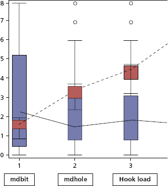
Figure 5.16 Box Plot for mdbit, mdhole, and hkldav
The length of the box equates to the difference between Q3 and Q1, which is IRQ. The line drawn inside the box is the median value. All data points above the top horizontal line or below the bottom horizontal line are treated as outliers.
Data were normalized to reduce unwanted variation between datasets. Normalization also enables data represented on different scales to be compared by converting them to a common scale.
As the total depth of each well drilled varies across the well portfolio, all parameters that are related to the depth (e.g., “hkldav,” “mdbit,” and “mdhole”) were normalized by dividing by the total depth of the chosen well. The unrelated parameters (e.g., “ropav”) were not normalized.
The second step of the approach is feature extraction, which is the transformation of patterns into features that are considered as a compressed representation.
As drilling time-series data represent a multidimensional input space, it is challenging to analyze owing to the large number of features that can be extracted from the raw data.3 To reduce the dimensionality of the data, a high-level representation is built where a set of significant features are calculated. These features provide an approximation of the original time-series data.
For each time-series variable Ti = {X1, X2, . . ., Xn}, i = 1..10 many statistical features were calculated to measure different properties of that variable. The main groups of the calculated statistical measures were:
- Measures of central tendency: mean, median, and mode
- Measures of variability: variance, standard deviation, IRQ, and range
- Measures of shape: skewness, kurtosis, and second moment
- Measures of position: percentiles
- Measures of impurity: entropy
High-dimensional data can contain a high degree of redundancy that adversely impact the performance of learning algorithms.4 Therefore, feature selection is an important step in the workflow. The initial step in the feature selection phase is removing the correlated features (collinearity) in order to reduce the dimensionality of the data and increase the computational efficiency. The most efficient method for feature selection is ranking the features with some statistical test, and then selecting the k features with the highest score or those with a score greater than some threshold t. Such univariate filters do not take into account feature interaction, but they allow a first inspection of the data and most probably provide reasonable results.5
Although the algorithms in Table 5.2 did not produce identical results, there was about 70 percent of similarity between these results. For example, most algorithms put flowin-p90, wobav-skewness, rpm-variance, and prespumpav-range features in the top of the ranking list.
Table 5.2 Feature-Ranking Algorithms
| Algorithm | Description |
| SAM | Calculates a weight according to “Significance Analysis for Microarrays” |
| PCA | Uses the factors of one of the principal components analyses as feature weights |
| SVM | Uses the coefficients of the normal vector of a linear support vector machine as feature weights |
| Chi-Squared | Calculates the relevance of a feature by computing for each attribute the value of the chi-squared statistic with respect to the class attribute |
| Relief | Measures the relevance of features by sampling examples and comparing the value of the current feature for the nearest example of the same and of a different class |
| Gini Index | Calculates the relevance of the attributes based on the Gini impurity index |
| Correlation | Calculates the correlation of each attribute with the label attribute and returns the absolute or squared value as its weight |
| Maximum Relevance | Selects Pearson correlation, mutual information, or F-test, depending on feature and label type |
| Uncertainty | Calculates the relevance of an attribute by measuring the symmetrical uncertainty with respect to the class |
The resulting question now is: How many features should be used to get the best model in terms of accuracy? To answer this question, it was imperative to conduct multiple tests. Many models with different numbers of features were developed, and subsequently an accuracy indicator was ascertained for each model.
A Principal Components Analysis (PCA) algorithm was used to rank the features. Features were added one at a time, starting with the top feature identified by the corresponding eigenvalues.
Once the most informative features have been extracted, the classification process is initiated. Five classification techniques were used in this study. These techniques are: Support Vector Machine (SVM),6 Artificial Neural Network (ANN),8 Rule Induction (RI), Decision Tree (DT), and Naïve Bayes (NB).
The performance of the classifiers was evaluated by using the cross-validation method. The worst classifier is invariably the NB, and the optimum classifiers are SVM and RI.
Unconventional Completion Best Practices
The objective of the study is to identify a completion strategy for an optimized hydraulic fracture treatment plan. Which variables will play the greatest part and impose an impact on hydrocarbon production volumes and post-treatment performance?
Workflows and models were developed capable of classifying a completion strategy and enumerating similar treatment plans previously performed in order to help engineers preclude potential challenges (similarity-based design). Additionally, the main factors influencing the treatment success or failure are identified.
- Prepare data: The dataset provided included multiple reservoirs and hydraulic fracture completion strategies. Owing to the inherent variability driven by reservoir parameters, a set of indicators have been developed to normalize the measurements with respect to reservoir parameters and other uncontrollable variables.
- Qualify completions: The treatments are grouped into bins of similarity to enable an exploration of the trends and hidden patterns that underpin the subsequent generation of models. Moreover, the grouping of completions serves to identify wells that are atypical for a cluster or cannot be assigned to a specific cluster and hence are deemed as outliers. These are then diagnosed as candidates for future investigation.
- Quantify completion grouping: Based on the indicators as defined in the first step, each completion can be classified to one of the bins as defined in the second step of the study. This allows engineers to classify new treatments based on analogs during the planning phase into their most likely bin in order to be able to identify similarities and foresee potential challenges.
- Deduce completion performance: Predictive models were developed to infer the most probable completion outcome in those bins where the number of measurements was sufficiently comprehensive to surface trends and relationships under uncertainty. The workflows and models are implemented for planning future wells by comparing the target reservoir properties to those in the extant completions data warehouse. We can then formulate a list of the most similar wells with the best performance to aid in the planning of new treatments.
The objectives of a data-driven model are common for both the planning and operational phases of a hydraulic fracture treatment strategy:
- Minimize total skin.
- Optimize fracture fluid volume.
- Optimize acid volume.
- Optimize proppant volume.
- Maximize cumulative hydrocarbons stage performance.
- Minimize sand and water stage production.
During the planning and operational phases we are studying those geologic parameters that characterize location optimization of a wellbore for maximum reservoir contact and hydrocarbon drainage:
- Perforation area and length
- Fracture dimensions
- Gross formation pay thickness
- Number of stages
- LaPlacian second derivative
- Dip
The planning phase must additionally consider the reservoir geomechanics and rock properties such as permeability and porosity. However, the study is primarily focused on identifying those controllable parameters that can be measured and understood to be effective to attain the previously listed objectives.
The fracture completion strategy is a multistage operation composed of several complex processes that can each result in failure or success. Figure 5.17 provides an overview of the complexity of a common fracture completion strategy.
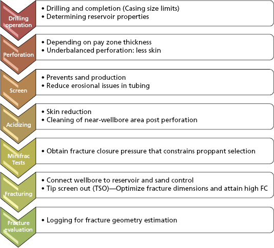
Figure 5.17 Complexity of a Hydraulic Fracture Completion Strategy
For high-permeability reservoirs short conductive fractures are ideal. When fracturing a high permeability formation, the fracture should be designed to extend beyond the external radius of the damaged region. Fractures that fail to extend beyond the damaged region will not improve production to optimum levels and will not significantly decrease the potential for sand production. Fractures that significantly extend beyond the damaged region will not significantly impact the productivity, but will result in higher stimulation costs.
Methodology
The investigated database contained 105 fracture pack completion treatments from 12 different reservoirs. The treatments were carried out on different well types (oil producer, gas producer, water injector). In this study we only focused on the treatments of the 67 oil producer wells, and divided the data into three buckets: static inputs, operationally controllable, and objective outputs as illustrated in Figure 5.18. Each treatment had 280 parameters grouped into the following sections:
- General
- Well and reservoir data
- Perforating information
- Post-perforating information
- Gravel pack (GP) packer information
- GP screen information
- Acidizing information
- Step rate test information
- Mini-fracture information
- Fracturing information
- Post-job analysis
- Completion and performance information
- Reservoir properties

Figure 5.18 Examples of the Datasets Studied
During the first step we differentiated between input and output parameters and filtered out those that have a minor or zero influence on the overall treatment success. Step rate and mini-fracture tests are essential for planning the treatment but do not directly impact the objective function.
SOMs are carried out with five variables at a time to investigate how reservoir parameters influence the fracture geometry. The examined variables are reservoir permeability, porosity, fracture length, fracture width, and fracture height. The goal was to figure out what kind of relationship exists between reservoir and fracture properties.
Based on the ontology, correlation matrixes were created to find an association between various input and output variables, and also among the output variables. The only strong correlation found was between flow efficiency and total skin, which resulted from the fact that the field engineers calculated the flow efficiency from the total skin. In Figure 5.19 the correlation matrix of the most important output variables is depicted.
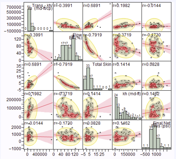
Figure 5.19 Correlation Matrix
To reduce the complexity and variance only the treatments on the oil producer wells were taken into account. The whole PCA analysis was done for 77 wells with 86 variables. With the first nine PCs 71 percent of the whole data behavior could be explained and the data complexity was reduced by 88 percent. However, the variables are not sorted by the criteria from the ontology.
During the first step the variables were normalized so that they were comparable to each other. The variable-importance workflow predicts those variables that play a significant role by evaluating the principal components.
Indicators were created to make observations comparable across different reservoirs in order to enable the extraction of patterns and rules. First we distinguished between controllable, uncontrollable, and output variables or objective functions.
For each stage of the completion strategy there are input indicators, which are the normalized design parameters. The output indicators are split in two main groups indicated by the color code. They represent the normalized reservoir response on each treatment stage and on the overall (total) success.
These indicators are listed below:
- Input indicators:
- Perforation
- In Perforation A = Perforation Length/Gross True Stratigraphic Thickness
- Acidizing
- In Acid A = Fluid Volume/(avg. Permeability∗Perforation Length MD)
- In Acid B = Acid Treating Pressure Gradient
- Fracturing
- In Fracture A = Final Pad Treating Pressure Gradient/BHPi Gradient
- In Fracture B = Final Fracture Treating Pressure Gradient/BHPi Gradient
- In Fracture C = Fracture Pad Fluid Volume/(avg. Perm∗Perforation Length MD)
- In Fracture D = Fracture Total Fluid Volume/(avg. Perm∗Perforation Length MD)
- In Fracture E = Fracture Pad Fluid Volume/Fracture Total Fluid Volume
- In Fracture F = Nr. of Stages
- In Fracture G = Max. Proppant Concentration
- Perforation
- Output indicators:
- Perforation
- Out Perforation A = (Perforation. OB/UB Pressure)/TVD
- Acidizing
- Out Acid B = (Final Injectivity Index-Initial Injectivity Index)/(Perforation Area∗(Initial Oil Rate/Transmissibility))
- Fracturing
- Out Fracture A = lbs/ft in TST Perforations
- Out Fracture B = Est Fracture Height
- Out Fracture C = Est Fracture Width
- Out Fracture D = Est. Fracture Length
- Out Fracture E = Est. CFD
- Total
- Total A = Initial Oil Rate/Transmissibility
- Total B = Net Pressure Gain/BHPi
- Total C = Flow Efficiency
- Total D = Total Skin
- Perforation
The PCA was repeated to qualify the correlations among the indicators. The first eight principal components were deemed as being an adequate representation of the variability. At this point, the first two principal components derived from the PCA on the indicators were taken to build the clusters so that the relationship among indicators and treatments can be qualified.
There are two main groups that can be identified easily as depicted in Figure 5.20. The one on the upper-right side behaves completely differently from the one on the bottom-left side. On the upper-right side are indicators that are mainly influenced by the fracturing design parameters. On the bottom-left side the main cluster can be divided into two further subclasses. The one with Clusters 3 and 5 includes the indicators that are mainly volume-related indicators and the other ones (Clusters 1 and 4) are mainly pressure related.
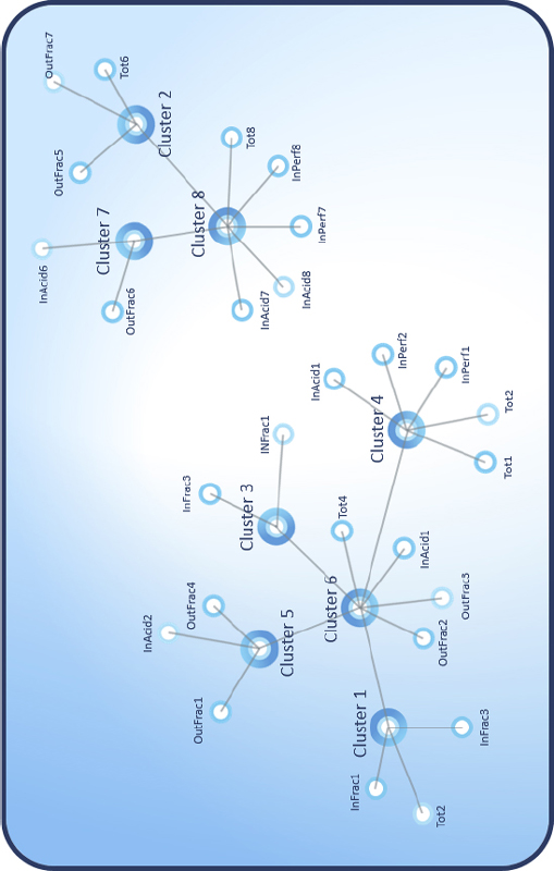
Figure 5.20 Oblique Clustering Results on the Indicators
Next, the oblique clustering was repeated, but now the treatments are also taken into account to see which treatment is best described by which indicator. After analyzing the result the same domination types could be discovered as in the first oblique clustering. However, there are some wells that could not be grouped into these domination types according to the first two principal components. They are the outliers and are neglected during subsequent investigation and model building.
A classification decision tree was built to quantify the domination types. The decision tree indicates that only three indicators (In Acid A, In Fracture E, and In Fracture A) are requisite to differentiate among the domination types.
In Acid 1, we see the strongest rule. It shows that if the relative acid volume pumped is over 1.6, then the well will reflect a volume domination type.
After that, the In Fracture E and In Fracture B differentiate between design- and pressure-dominated treatments. Note that there are two subgroups of design-dominated and three subgroups of pressure-dominated treatments.
After analyzing the data and merging with expert knowledge from the oil industry a model was built that classifies the existing treatments into several categories according to their design and performance. The outcome is a list of type wells for each category. This model can be used for planning future wells by comparing its reservoir properties to the ones in the existing database. It can then generate the list of the most similar wells (based on the uncontrollable variables) with the best performance. The scheme of the type of wells can be used as a design outline by the planning engineers.
Chapter 8’s “Pinedale Asset” details another example of a completion optimization strategy ascertained via an advanced analytical methodology. This examination was carried out in the unconventional asset known as the Pinedale in Western Wyoming.