
HDR Multiview Image Sequence Generation
Toward 3D HDR Video
R.R. Orozco*; C. Loscos†; I. Martin*; A. Artusi* * University of Girona, Girona, Spain
† University of Reims Champagne-Ardennes, Reims, France
Abstract
High dynamic range (HDR) imaging and stereoscopic 3D are active research fields, with challenges posed in various directions: acquisition, processing, and display. This chapter analyzes the latest advances in stereo HDR imaging acquisition from multiple exposures, in order to highlight the current progress toward a common target: stereoscopic 3D HDR video. A method to build multiscopic HDR images from low dynamic range (LDR) multiexposures is proposed. This method is based on a patch-match algorithm which has been adapted and improved to take advantage of epipolar geometry constraints of stereo images. Experimental results show accurate matching between stereo images that allow generating HDR for each LDR view of the sequence.
Keywords
Multiexposure HDR generation; Stereoscopic high-dynamic range; Multiexposure stereo matching; Video HDR
1 Introduction
High dynamic range (HDR) content generation has been recently moving from the 2D to 3D imaging domain, introducing a series of open problems that need to be solved. Three-dimensional images are displayed in two main ways: either from two views for monoscopic displays with glasses, or from multiple views for auto-stereoscopic displays. Most current auto-stereoscopic displays accept from five to nine different views [1]. To our knowledge, HDR auto-stereoscopic displays do not exist yet. However, HDR images are device independent, they store values from the scene they represent independently of the device that will project them. Actually, HDR images existed long before the first HDR prototype appeared. Similarly to displaying tone-mapped HDR images on low dynamic range (LDR) displays, it is possible to feed LDR auto-stereoscopic displays with tone-mapped HDRs, one per each view required by the display.
Some of the techniques used to acquire HDR images from multiple LDR exposures have been recently extended for multiscopic images [2–10]. However, most of these solutions suffer from a common limitation: they rely on accurate dense stereo matching between images that is not robust in case of brightness difference between exposures [11].
This chapter presents a solution to combine sets of multiscopic LDR images into HDR content using image correspondences based on the Patch-Match algorithm [12]. This algorithm was recently used by Sen et al. [13] to build HDR images preventing from significant ghosting effects. Furukawa and Ponce [14] noticed the importance of improving the coherence of neighboring patches, an issue tackled in this chapter. Their results were promising for multiexposure sequences where the reference image is moderately underexposed or saturated, but it fails when the reference image has large underexposed or saturated areas.
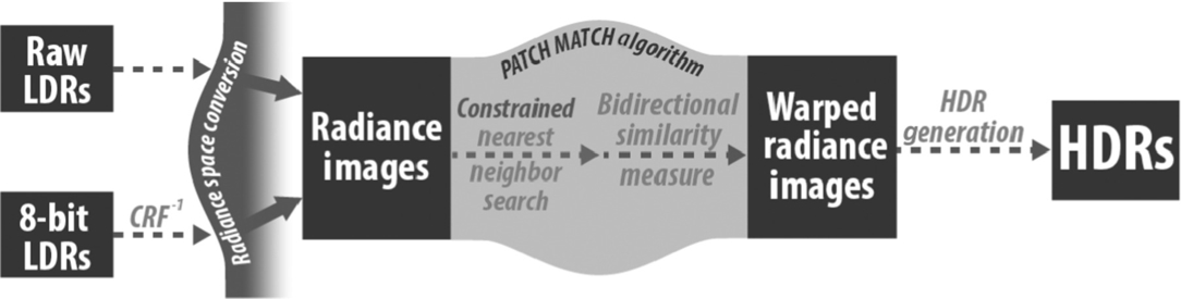
The method described in this chapter improves [12] the approach for multiscopic image sequences (Fig. 1). It also reduces the search space in the matching process and improves the incoherence of the matches in the original algorithm. Each image in the set of multiexposed images is used as a reference; we look for matches in all the remaining images. Accurate matches allow us to synthesize a set of HDR images, one for each view used for HDR merging.
The main contributions of this chapter can be summarized as follows:
• We provide an efficient solution to multiscopic HDR image generation.
• Traditional stereo matching produces several artifacts when directly applied on images with different exposures. We introduce the use of an improved version of patch match to solve these drawbacks.
• Patch-match algorithm was adapted to take advantage of the epipolar geometry reducing its computational costs while improving its matching coherence drawbacks.
1.1 Stereoscopic Imaging
Apart from a huge amount of colors and fine details, our visual system is able to perceive depth and 3D shape of objects. Digital images offer a representation of reality projected in 2D arrays. We can guess the distribution of objects in depth because of monoscopic cues like perspective, but we cannot actually perceive depth in 2D images. Our brain needs to receive two slightly different projections of the scene to actually perceive depth.
Stereoscopy is any imaging technique which enhances or enables depth perception using the binocular vision cues [15]. Stereo images refer to a pair of images horizontally aligned and separated at a scalable distance similar to the average distance between human eyes. The different available stereo display systems project them in a way such that each eye perceives only one of the images. In recent years, technologies like stereoscopic cameras and displays have become available to consumers [16–18]. Stereo images require recording at minimum, two views of a scene, one for each eye. However, depending on the display technology, it could be more. Some auto-stereoscopic displays render more than nine different views for an optimal viewing experience [1].
Some prototypes were proposed to acquire stereo HDR content from two or more differently exposed views. Most approaches [2–5, 8, 19, 20] are based on a rig of two cameras placed like a conventional stereo configuration that captures different exposed images. The next sections offer a background of the geometry of stereo systems (Section 1.2) as well as a survey on the different existing approaches for multiscopic HDR acquisition (Section 2).
1.2 Epipolar Geometry
One of the most popular topics of research in computer vision is stereo matching, which refers to the correspondence between pixels of stereo images. The geometry that relates 3D objects to their 2D projection in stereo vision is known as epipolar geometry. It explains how the stereo images are related and how depth can mathematically be retrieved from a pair of images.
Fig. 2 describes the main components of the epipolar geometry. A point x in the 3D world coordinates is projected onto the left and right images IL and IR, respectively. cL and cR are the two centers of projection of the cameras, the plane formed by them, and the point x is known as the epipolar plane. xL and xR are the projections of x in IL and IR, respectively.
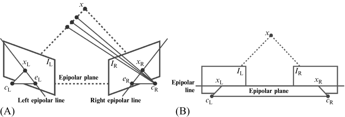
For any point xL in the left image, the distance to x is unknown. According to the epipolar geometry, the corresponding point xR is located somewhere on the right epipolar line. Epipolar geometry does not mean direct correspondence between pixels. However, it reduces the search for a matching pixel to a single epipolar line. The accurate position of a point in the space requires the correct matches between the two images, the focal length, and the distance between the two cameras. Otherwise, only relative measures can be approximated.
If the image planes are aligned and their optical axes are parallel, the two epipolar lines (left and right) converge. In such a case, correspondent pixels rely on the same epipolar line in both images, which simplifies the matching process. Aligning the cameras to force this configuration might be difficult, but images can be aligned.
This alignment process is known as rectification. After the images are rectified, the search space for a pixel match is reduced to the same row, which is the epipolar line. To the best of our knowledge, all methods in stereo HDR are based on rectified images and they take advantage of the epipolar constrain during the matching process. Rectified image sets are available on the Internet for testing purposes, like Middlebury [21].
If corresponding pixels (matches) are on the same row on both images, it is possible to define the difference between the images by the horizontal distance between matches in the two images. The image that stores all the horizontal shifts between stereo pairs is called disparity maps.
Despite epipolar geometry simplifying the problem, it is far from being solved. Determining pixel matches in regions of similar color is a difficult problem. Moreover, the two views correspond to different projections of the scene, which means that occlusion takes place between objects. The HDR context adds the fact that different views might be differently exposed, reducing the possibilities of finding color consistent matches.
2 Multiple Exposure Stereo Matching
Stereo matching (or disparity estimation) is the process of finding the pixels in the different views that correspond to the same 3D point in the scene. The rectified epipolar geometry simplifies this process to find correspondences on the same epipolar line. It is not necessary to calculate the 3D point coordinates to find the correspondent pixel on the same row of the other image. The disparity is the distance d between a pixel and its horizontal match in the other image.
Akhavan et al. [20, 22] compared the different ways to obtain disparity maps from HDR, LDR, and tone-mapped stereo images. A useful comparison among them is offered and illustrates that the type of input has a significant impact on the quality of the resulting disparity maps.
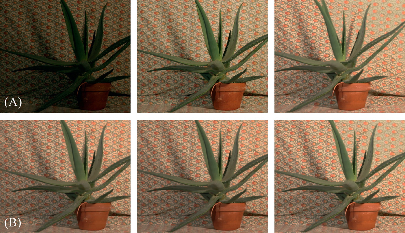
Fig. 3 shows an example of a differently exposed multiview set corres- ponding to one frame in a multiscopic system of three views. The main goal of stereo matching is to find the correspondences between pixels to generate one HDR image per view for each frame.
Correspondence methods rely on matching cost functions to compute the color similarity between images. It is important to consider that the exposure difference needs to be compensated. Even using radiance space images where pixels are supposed to have the same value for same points in the scene, there might be brightness differences. Such differences may be introduced by the camera due to image noise, slightly different settings, vignetting, or caused by inaccuracies in the estimated CRF. For good analysis and comparison of the existing matching costs and their properties, refer to [9, 11, 23, 24].
Different approaches exist to recover HDR from multiview and multiexposed sets of images. Some of them [3–5] share the same pipeline as in Fig. 4. All mentioned works take as input a set of images with different exposures acquired using a camera with unknown response function. In such cases, the disparity maps need to be calculated in the first instance using the LDR pixel values. Matching images under important differences of brightness is still a big challenge in computer vision.

2.1 Per Frame CRF Recovery Methods
To our knowledge, Troccoli et al. [3] introduced the first technique for HDR recovery from multiscopic images of different exposures. They observed that normalized cross correlation (NCC) is approximately invariant to exposure changes when the camera has a gamma response function. Under such an assumption, they use the algorithm described by Kang and Szeliski [25] to compute the depth maps that maximizes the correspondence between 1 pixel and its projection in the other image. The original approach [25] used sum of squared differences (SSD), but it was substituted by NCC in this work.
Images are warped to the same viewpoint using the depth map. Once pixels are aligned, the CRF is calculated using the method proposed by Grossberg and Nayar [26] over a selected set of matches. With the CRF and the exposure values, all images are transformed to radiance space and the matching process is repeated, this time using SSD. The new depth map improves the previous one and helps to correct artifacts. The warping is updated and HDR values are calculated using a weighted average function.
The same problem was addressed by Lin and Chang [4]. Instead of NCC, they use scale-invariant feature transform (SIFT) descriptors to find matches between LDR stereo images. SIFT is not robust under different exposure images. Only the matches that are coherent with the epipolar and exposure constraints are selected for the next step. The selected pixels are used to calculate the CRF.
The stereo matching algorithm they propose is based on a previous work [27]. Belief propagation is used to calculate the disparity maps. The stereo HDR images are calculated by means of a weighted average function. Even using the best results only, SIFT is not robust enough under significant exposure variations.
A ghost removal technique is used afterward to tackle the artifacts, due to noise or stereo mismatches. The HDR image is exposed to the best exposure of the sequence. The difference between them is calculated and pixels over a threshold are rejected considering them like mismatches. This is risky because HDR values in areas under- and overexposed in the best exposure may be rejected. In this case ghosting would be solved, but LDR values may be introduced in the resulting HDR image.
Sun et al. [5] (inspired by Troccoli et al. [3]) follow the pipeline described in Fig. 4 too. They assume that the disparity map between two rectified stereo images can be modeled as a Markov random field. The matching problem is presented like a Bayesian labeling problem. The optimal disparity values are obtained by minimizing an energy function.
The energy function they use is composed of a pixel dissimilarity term (NCC in their solution) and a disparity smoothness term. It is minimized using the graph cut algorithm to produce initial disparities. The best disparities are selected to calculate the CRF with the algorithm proposed by Mitsunaga and Nayar [28].
Images are converted to radiance space and then another energy minimization is executed to remove artifacts. This time the pixel dissimilarity cost is computed using the Hamming distance between candidates.
The methods presented up to this point have a high computational cost. Calculating the CRF from nonaligned images may introduce errors because the matching between them may not be robust. Two exposures are not enough to obtain a robust CRF with existing techniques. Some of them execute two passes of the stereo matching algorithm, the first one to detect matches for the CRF recovery and a second one to refine the matching results. This might be avoided by calculating the CRF in a previous step using multiple exposures of static scenes. Any of the available techniques [26, 28–30] can be used to get the CRF corresponding to each camera. The curves help to transform pixel values into radiance for each image and the matching process is executed in radiance space images. This avoids one stereo matching step and prevents errors introduced by disparity estimation and image warping.
Rufenacht [19] proposes two different ways to obtain stereoscopic HDR video content. The first, a temporal approach, where exposures are captured by temporally changing the exposure time of two synchronized cameras to get two frames of the same exposure per shot. And the second, a spatial approach, where cameras have different exposure times for all the shots so the two frames of the same shot are exposed differently.
2.2 Offline CRF Recovery Methods
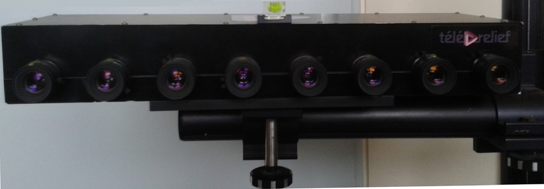
Bonnard et al. [7] propose a methodology to create content that combines depth and HDR video for auto-stereoscopic displays. Instead of varying the exposure times, they use neutral density filters to capture different exposures. A camera with eight synchronized objectives and three pairs of 0.3, 0.6, and 0.9 filters, plus two nonfiltered views provide eight views with four different exposures of the scene stored in 10-bit RAW files. They use a geometry-based approach to recover depth information from epipolar geometry. Depth maps drive the pixel match procedure.
Bätz et al. [2] present a work flow for disparity estimation, divided in the following steps:
• Cost initialization consists of evaluating the cost function, Zero NCC in this case, for all values within a disparity search range.
The matching is performed on the luminance channel of radiance space image using patches of 9 × 9 pixels. The result of searching for disparities is the disparity space image (DSI), a matrix of m × n × d + 1 for an images of m × n pixels with d + 1 being the disparity search range.
• Cost aggregation smoothes the DSI and finds the final disparity of each pixel in the image. They use an improved version of the cross-based aggregation method described by Mei et al. [31]. This step is performed, not in the luminance channel like in the previous step, but in the actual RGB images.
• Image warping is in charge of actually shifting all pixels according to their disparities. Dealing with occluded areas between the images is the main challenge in this step. The authors propose to do the warping in the original LDR images which adds a new challenge: dealing with under- and overexposed areas. A backward image warping is chosen to implicitly ignore the saturation problems. The algorithm produces a new warped image with the appearance of the reference one by using the target image and the corresponding disparity map. Bilinear interpolation is used to retrieve values at subpixel precision.
Selmanovic et al. [10] propose to generate stereo HDR video from a pair of HDR and LDR videos, using an HDR camera [32] and a traditional digital camera (Canon 1Ds Mark II) in stereo configuration. This chapter is an extension to video of a previous one [15] focused only on stereo HDR images. In this case, one HDR view needs to be reconstructed from two different sources.
Their method proposes three different approaches to generate the HDR:
1. Stereo correspondence: It is computed to recover the disparity map between the HDR and the LDR images. The disparity map allows us to transfer the HDR values to the LDR image. The sum of absolute differences (SAD) is used as a matching cost function. Both images are transformed to lab color space, which is perceptually more accurate than RGB.
The selection of the best disparity value for each pixel is based on winner takes all technique. The lower SAD value is selected in each case. An image warping step based on Fehn [33] is used to generate a new HDR image corresponding to the LDR view. The SAD stereo matcher can be implemented to run in real time, but the resulting disparity maps could be noisy and not accurate. The over- and underexposed pixels may end up in a wrong position. In large areas of the same color and hence same SAD cost, the disparity will be constant. Occlusions, reflective or specular objects may cause some artifacts.
2. Expansion operator: It could be used to produce an HDR image from the LDR view. Detailed state-of-the-art reports on LDR expansion were previously published [34, 35]. However, in this case, we need the expanded HDR to remain coherent with the original LDR. Inverse tone mappers are not suitable because the resulting HDR image may be different from the acquired one, producing results not possible to fuse through a common binocular vision.
They propose an expansion operator based on a mapping between the HDR and the LDR image, using the first one as reference. A reconstruction function maps LDR to HDR values (Eq. 1) based on an HDR histogram with 256 bins, putting the same number of HDR values in each bin, as there are in the LDR histogram.
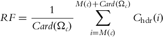
In Eq. (1), Ωc = {j = i…N : cldr(j) = c}, c = 0.255 is the index if a bin Ωc, Card(⋅) returns the number of elements in the bin, N is the number of pixels in the image, cldr(j) are the intensity values for the pixel j, ![]() is the number of pixels in the previous bin, and chdr are the intensities of all HDR pixels sorted ascending. RF is used to calculate the look-up table and afterward expansion can be performed directly assigning the corresponding HDR value to each LDR pixel.
is the number of pixels in the previous bin, and chdr are the intensities of all HDR pixels sorted ascending. RF is used to calculate the look-up table and afterward expansion can be performed directly assigning the corresponding HDR value to each LDR pixel.
The expansion runs in real time, is not view dependent, and avoids stereo matching. The main limitation is again on saturated regions.
3. Hybrid method combines the two previous ones. Two HDR images are generated using the previous approaches (stereo matching and expansion operator). Pixels in well-exposed regions are expanded using the first method (expansion operator), while matches for pixels in under- or overexposed regions are found using SAD stereo matching adding a correction step. A mask of under- and oversaturated regions is created, using a threshold for pixels over 250 or below 5. The areas out of the mask are filled in with the expansion operator while the under- or overexposed regions are filled in with an adapted version of the SAD stereo matching to recover more accurate values in over- or underexposed regions.
Instead of having the same disparity over the whole under- or overexposed region, this variant interpolates disparities from well-exposed edges. Edges are detected using a fast morphological edge detection technique described by Lee et al. [36]. Even though some small artifacts may still be produced by the SAD stereo matching in such areas.
Orozco et al. [37] presented a method to generate multiscopic HDR images from LDR multiexposure images. They adapted a patch-match approach [13] to find matches between stereo images using epipolar geometry constrains. This method reduces the search space in the matching process, and includes an improvement of the incoherence problem described for the patch-match algorithm. Each image in the set of multiexposed images is used as a reference, looking for matches in all the remaining images. These accurate matches allow us to synthesize images corresponding to each view, which are merged into one HDR per view that can be used in auto-stereoscopic displays.
3 Patch-Based Multiscopic HDR Generation
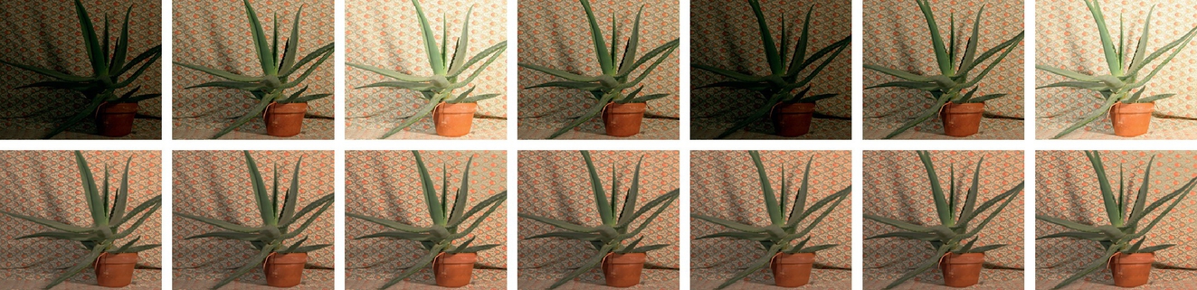
The input for multiscopic HDR is a sequence of LDR images (formed of RAW or 8-bit RGB data) as shown in the first row of Fig. 5. Each image is acquired from a different viewpoint, usually from a rig of cameras in a stereo distribution, or multiview cameras (see Fig. 6). If the input images are in a 8-bit format, an inverse CRF needs to be recovered for each camera involved in the acquisition. This calibration step is performed only once, using a static set of images for each camera. The inverse of the CRFs is used to transform the input into radiance space. The remaining steps are performed using radiance space values instead of RGB pixels.
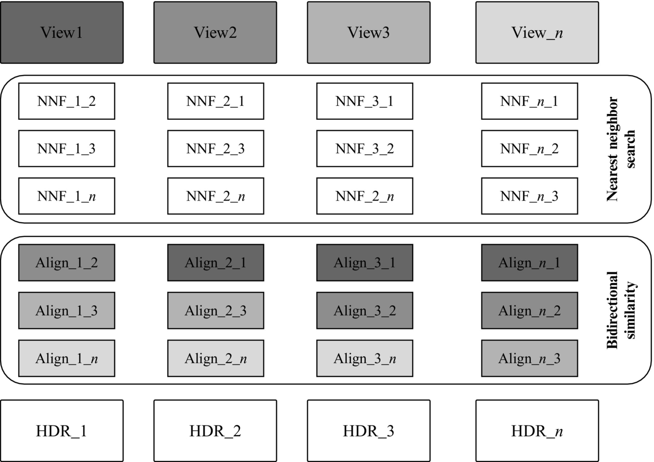
An overview of our framework is shown in Fig. 1. The first step is to recover the correspondences between the n images of the set. We propose to use a nearest neighbor search algorithm (see Section 3.1) instead of a traditional stereo matching approach. Each image acts like a reference for the matching process. The output of this step is n − 1 warped images for each exposure. Afterward, the warped images are combined into an output HDR image for each view (see Section 3.2).
3.1 Nearest Neighbor Search
For a pair of images Ir and Is, we compute a nearest neighbor field (NNF) from Ir to Is using an improved version of the method presented by Barnes et al. [12]. NNF is defined over patches around every pixel coordinate in image Ir for a cost function D between two patches of images Ir and Is. Given a patch coordinate r ∈ Ir and its corresponding nearest neighbor s ∈ Is, NNF(r) = s. The values of NNF for all coordinates are stored in an array with the same dimensions as Ir.
We start initializing the NNFs using random transformation values within a maximal disparity range on the same epipolar line. Consequently the NNF is improved by minimizing D until convergence or a maximum number of iterations is reached. Two candidate sets are used in the search phase as suggested by Barnes et al. [12]:
1. Propagation uses the known adjacent nearest neighbor patches to improve NNF. It quickly converges, but it may fall in a local minimum.
2. Random search introduces a second set of random candidates that are used to avoid local minimums. For each patch centered in pixel v0, the candidates ui are sampled at an exponentially decreasing distance vi previously defined by Barnes et al.:
where Ri is a uniform random value in the interval [−1, 1], w is the maximum value for disparity search, and α is a fixed ratio (1/2 is suggested).
Taking advantage of the epipolar geometry, both search accuracy and computational performance are improved. Geometrically calibrated images allow us to reduce the search space from 2D to 1D domain, consequently reducing the search domain. The random search of matches only operates in the range of maximum disparity in the same epipolar line (1D domain), avoiding a search in 2D space. This significantly reduces the number of samples to find a valid match.
However, the original NNFs approach [12] used in the patch-match algorithm has two main disadvantages, the lack of completeness and coherency. These problems are illustrated in Fig. 7 and the produced artifact in Fig. 8. The lack of coherency refers to the fact that two neighbor pixels in the reference image may match two separated pixels in the source image, like in Fig. 7A. Completeness issues refer to more than 1 pixel in the reference image matching the same correspondence in the source image, as shown in Fig. 7B.
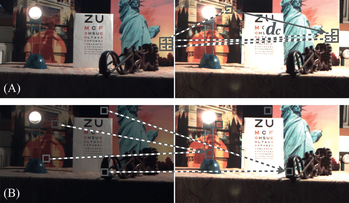
To overcome this drawback, we propose a new distance cost function D by incorporating a coherence term to penalize matches that are not coherent with the transformation of their neighbors. Both Barnes et al. [12] and Sen et al. [13] use the SSD described in Eq. (4) where T represents the transformation between patches of N pixels in images Ir and Is. We propose to penalize matches with transformations that differ significantly from it neighbors by adding the coherence term C defined in Eq. (5). The variable dc represents the Euclidean distance to the closest neighbor’s match and Maxdisp is the maximum disparity value. This new cost function forces pixels to preserve coherent transformations with their neighbors.
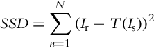
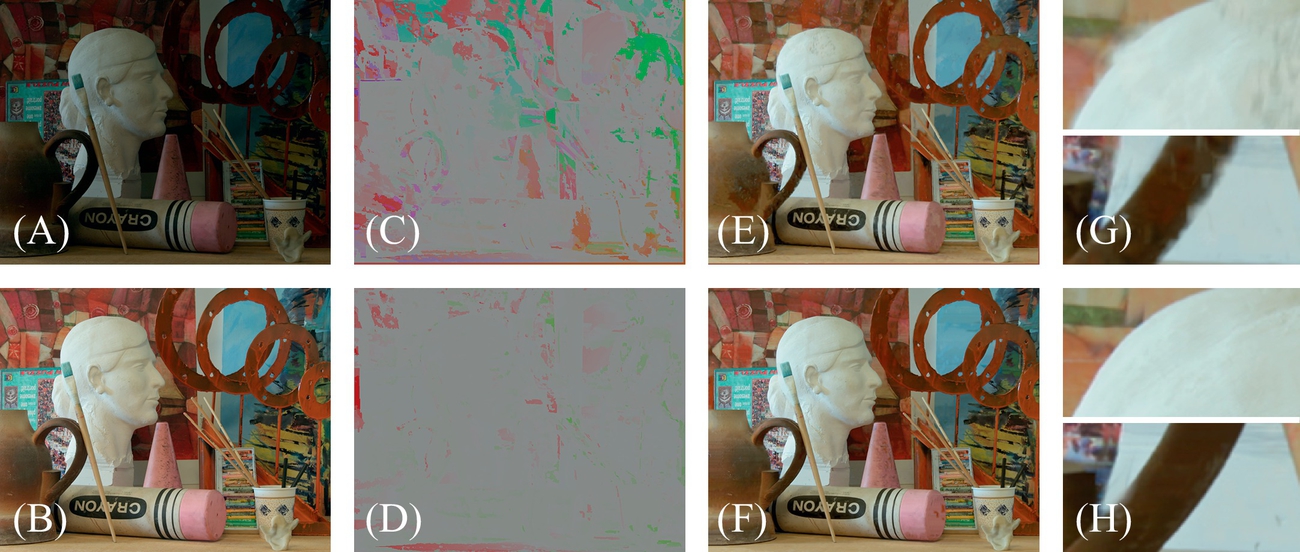
Fig. 8D and F corresponds to the results including the improvements presented in this section. Fig. 8C and D shows a color mentioned of the NNFs using HSV color space. The magnitude of the transformation vector is visualized in the saturation channel and the angle in the hue channel. Areas represented with the same color in the NNF color mentioned mean similar transformation. Objects in the same depth may have similar transformation. Notice that the original Patch Match [12] finds very different transformations for neighboring pixels of the same objects and produces artifacts in the synthesized image.
3.2 Image Alignment and HDR Generation
The nearest neighbor search step finds correspondences among all the different views. The matches are stored in a set of n2 − n NNFs. This information allows to generate n − 1 images with different exposures realigned on each view. The set of aligned multiple exposures per view feeds the HDR generation algorithm to produce an HDR image for every view (see Fig. 9).
Despite the improvements in the cost function presented in the previous section, NNF may not be coherent in occluded or saturated areas. However, even in such cases, a match to a similar color is found between each pair of images Ir;Is. This makes it possible to synthesize images for each exposure corresponding to each view.
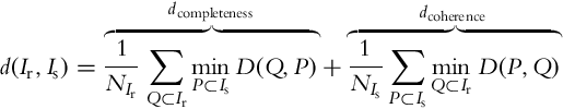
Direct warping from the NNFs is an option, but it may generate visible artifacts as shown in Fig. 10. We use Bidirectional Similarity Measure (BDSM) (Eq. 6), proposed by Simakov et al. [38] and used by Barnes et al. [12], which measures similarity between pairs of images. The warped images are generated as an average of the patches that contribute to a certain pixel. It is defined in Eq. (6) for every patch Q![]() and P
and P![]() , and a number N of patches in each image, respectively. It consists of two terms: coherence that ensures that the output is geometrically coherent with the reference and completeness that ensures that the output image maximizes the amount of information from the source image:
, and a number N of patches in each image, respectively. It consists of two terms: coherence that ensures that the output is geometrically coherent with the reference and completeness that ensures that the output image maximizes the amount of information from the source image:
This improves the results by using bidirectional NNFs (![]() and backward,
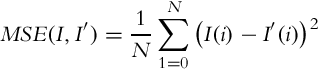
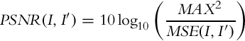
and backward, ![]() ). It is more accurate to generate images using only two iterations of nearest neighbor search and bidirectional similarity, than four iterations of neighbor search and direct warping. Table 1 shows some values of mean squared error (MSE) and peak signal-to-noise ratio (PSNR) of images warped like the ones in Fig. 10 comparing to the reference LDR image. The values in the table corresponds to the average MSE and PSNR calculated per each channel of the images in L*a*b* color space, using Eqs. (7) and (8), respectively.
). It is more accurate to generate images using only two iterations of nearest neighbor search and bidirectional similarity, than four iterations of neighbor search and direct warping. Table 1 shows some values of mean squared error (MSE) and peak signal-to-noise ratio (PSNR) of images warped like the ones in Fig. 10 comparing to the reference LDR image. The values in the table corresponds to the average MSE and PSNR calculated per each channel of the images in L*a*b* color space, using Eqs. (7) and (8), respectively.
Table 1
Direct vs bidirectional warping
| Direct warp | Bidirectional | |||
| Iterations | MSE | PSNR | MSE | PSNR |
| 1 | 2.42199 | 41.8613 | 2.17003 | 42.3734 |
| 2 | 2.40966 | 41.8764 | 2.17195 | 42.3762 |
| 4 | 2.4137 | 41.8728 | 2.16708 | 42.3846 |
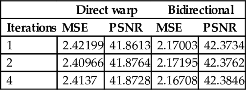
Because the matching is totally independent for pairs of images, it was implemented in parallel. Each image matches the remaining other views. This produces n − 1 NNFs for each view. The NNFs are, in fact, the two components of the BDSM of Eq. (6). The new image is the result of accumulating pixel colors of each overlapping neighbor patch and averaging them.
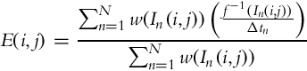
The HDR images (one HDR per view) are generated using a standard weighted average [28–30] as defined in Eq. (9) and the weighting function of Eq. (10) proposed by Khan et al. [39] where In represents each image in the sequence, w corresponds to the weight, f is the CRF, Δtn is the exposure time for the Ith image of the sequence.
4 Results and Discussion
Five datasets were selected in order to demonstrate the robustness of our results. For the set “Octocam” all the objectives capture the scene at the same time and synchronized shutter speed. For the rest of the datasets, the scenes are static. This avoids the ghosting problem due to dynamic objects in the scene. In all figures of this section, we use the different LDR exposures for display purposes only, the actual matching is performed in radiance space.
The “Octocam” dataset are eight RAW images with 10-bit of color depth per channel. They were acquired simultaneously using the Octocam [40] with a resolution of 748 × 422 pixels. The Octocam is a multiview camera prototype composed by eight objectives horizontally disposed. All images are taken at the same shutter speed (40 ms), but we use three pairs of neutral density filters that reduce the exposure dividing by 2, 4, and 8, respectively. The exposure times for the input sequence are equivalent to 5, 10, 20, and 40 ms, respectively [7]. The objectives are synchronized so all images correspond to the same time instant.
The sets “Aloe,” “Art,” and “Dwarves” are from the Middlebury website [21]. We selected images that were acquired under fixed illumination conditions with shutter speed values of 125, 500, and 2000 ms for “Aloe” and “Art” and values of 250, 1000, and 4000 ms for “Dwarves.” They have a resolution of 1390 × 1110 pixels and were taken from three different views. Even if we have only three different exposures, we can use the seven available views by alternating the exposures as shown in Fig. 14.
The last two datasets were acquired from two of the state-of-the-art papers. Bätz et al. [2] shared their image dataset (IIS Jumble) at a resolution of 2560 × 1920 pixels. We selected five different views from their images. They were acquired at shutter speeds of 5, 30, 61, 122, and 280 ms, respectively. Pairs of HDR images like the one in Fig. 11, both acquired from a scene and synthetic examples, come from Selmanovic et al. [10]. For 8-bit LDR datasets, the CRF is recovered using a set of multiple exposure of a static scene. All LDR images are also transformed to radiance space for fair comparison with other algorithms.
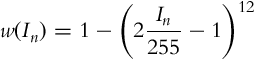
Fig. 11 shows a pair of images linearized from HDR images courtesy of Selmanovic et al. [10] and the comparison between the original PM from Barnes et al. [12] and our method, including the coherence term and epipolar constrains. The images in Fig. 11B and F represent the NNF. They are encoded into an image in HSV color space. Magnitude of the transformation vector is visualized in the saturation channel and the angle in the hue channel. Notice that our results represent more homogeneous transformations, represented in gray color. Images in Fig. 11C and G are synthesized result images for the Ref image obtained using pixels only from the Src image. The results correspond to the same number of iterations (two in this case). Our implementation converges faster producing accurate results in less iterations than the original method.
All the matching and synthesizing processes are performed in radiance space. They were converted to LDR using the corresponding exposure times, and the CRF for display purposes only. The use of an image synthesis method like the BDSM instead of traditional stereo matching allows us to synthesize values also for occluded areas.
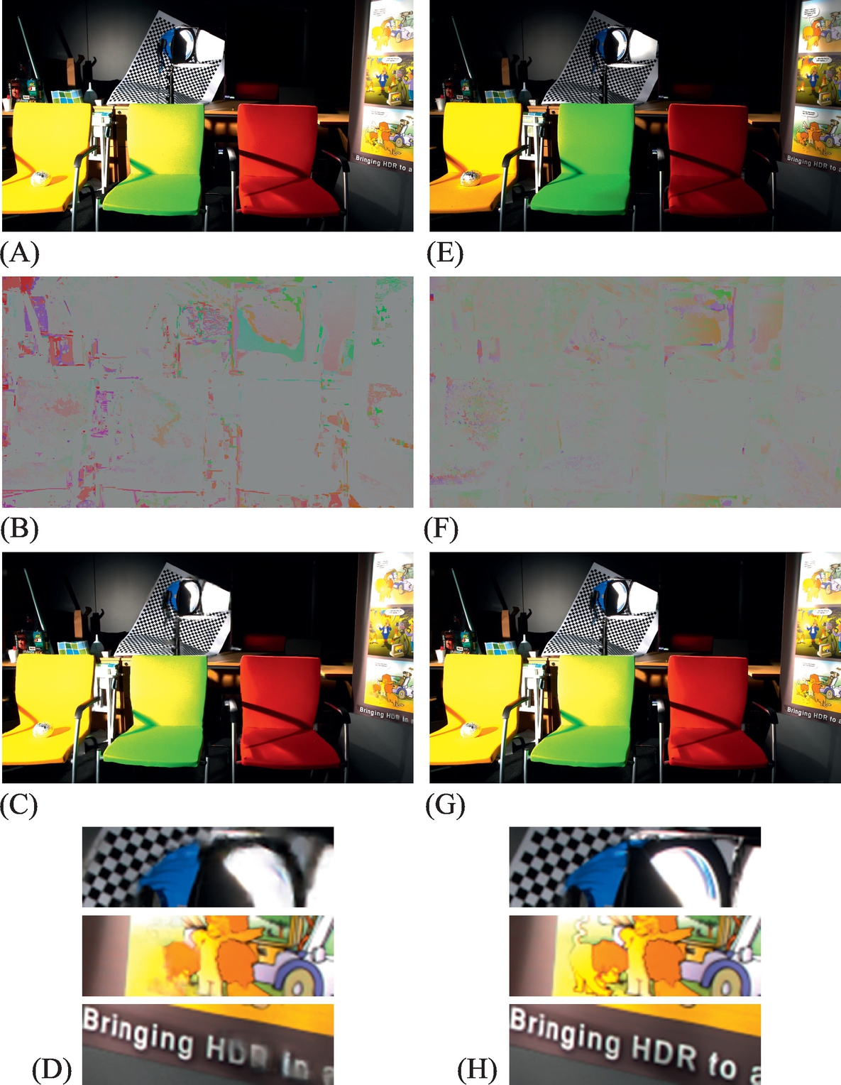
Fig. 12 shows the NNFs and the images synthesized for different iterations of both our method and the original patch match. Our method converges faster and produces more coherent results than Barnes et al. [12]. In occluded areas, the matches may not be accurate in terms of geometry due to the lack of information. Even in such cases, the result is accurate in terms of color. After several tests, only two iterations of our method were enough to get good results while five iterations were recommended for previous approaches.
Fig. 13 shows one example of the generated HDR corresponding to the lowest exposure LDR view in the IIS Jumble dataset. It is the result of merging all synthesized images obtained with the first view as reference. The darker image is also the one that contains more noisy and underexposed areas. HDR values were recovered even for such areas and no visible artifacts appears. On the contrary, the problem of recovering HDR values for saturated areas in the reference image remains unsolved. When the dynamic range differences are extreme, the algorithm does not provide accurate results. Future work must provide new techniques, because the lack of information inside saturated areas does not allow patches to find good matches.
The inverse CRFs for the LDR images were calculated from a set of aligned multiexposed images using the software RASCAL, provided by Mitsunaga and Nayar [28]. Fig. 14 shows the result of our method for a whole set of LDR multiview and differently exposed images. All obtained images are accurate in terms of contours, no visible artifacts compared to the LDR were obtained.
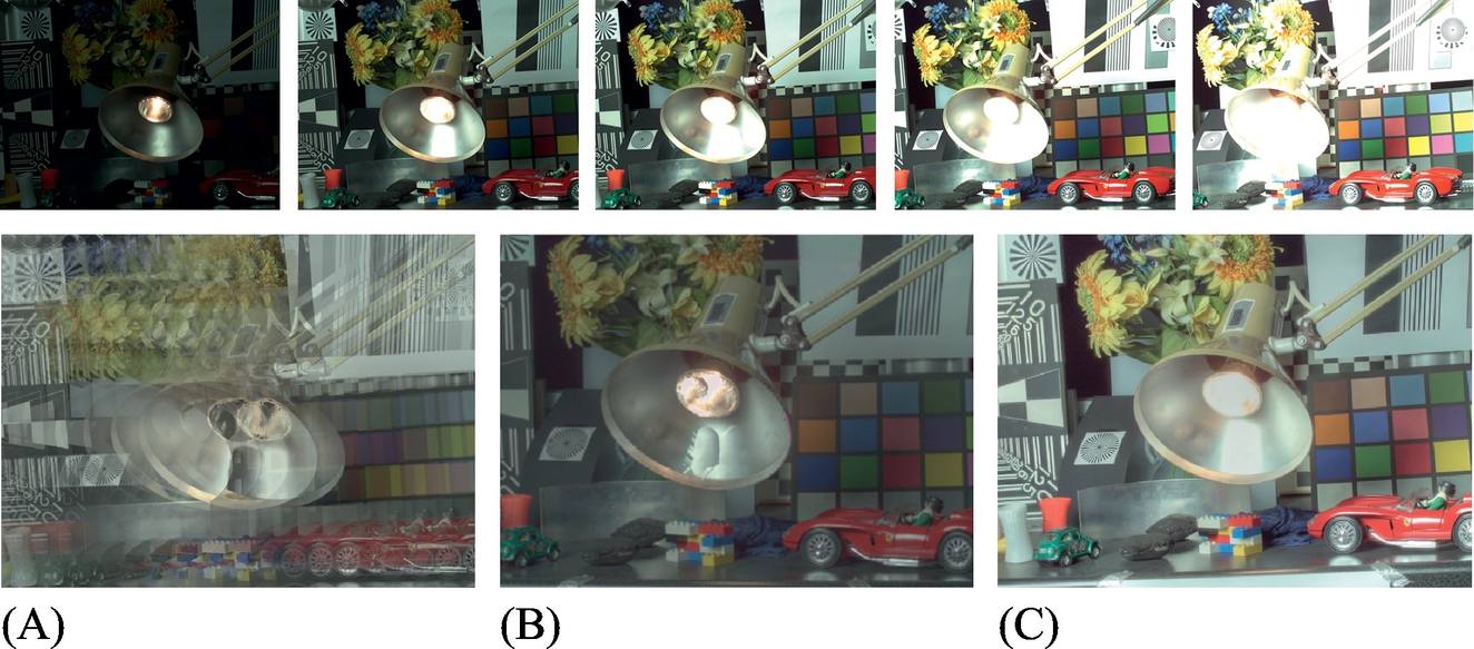
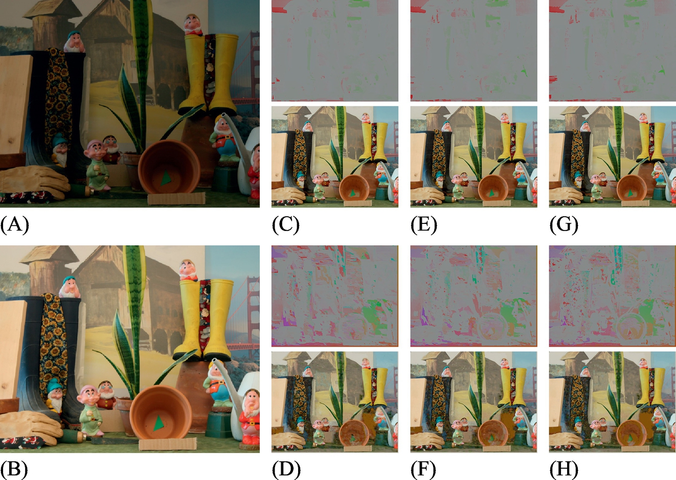
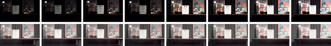
Fig. 15 shows the result of the proposed method in a scene with important lighting variations. The presence of the light spot introduces extreme lighting differences between the different exposures. For bigger exposures, the light glows from the spot and saturates pixels, not only inside the spot, but also around it. There is not information in saturated areas and the matching algorithm does not find good correspondences. The dynamic range is then compromised in such areas and they remain saturated.
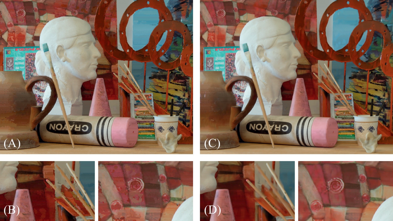
Two of the datasets used in the tests provide aligned multiple exposures for each view, which allows us to generate ground truth HDR images per view. Fig. 16 shows the results of comparing some of our results to ground truth images using the HDR-VDP-2 metric proposed by Mantiuk et al. [41]. This metric provides some values to describe how similar two HDR images are.
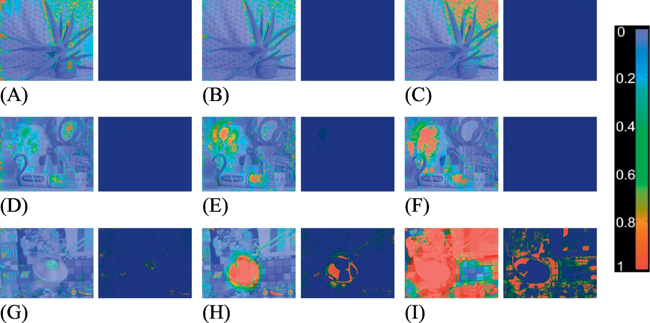
The quality correlate Q is 100 for the best quality and gets lower for lower quality. Q can be negative in case of very large differences. The images at the right of each pairs in Fig. 16 are the probability of detection map. It shows where and how likely a difference will be noticed. However, it does not show what this difference is. Images at the left on each pair show the contrast-normalized per-pixel difference weighted by the probability of detection. The resulting images do not show probabilities. However, they better correspond to the perceived differences.
The results illustrate that in general, no differences are perceived. Except in areas that appear totally saturated in the reference image, like the head of the sculpture in the “Art” dataset or the lamp in the IIS Jumble. In such cases visible artifact appears because the matching step fails to find valid correspondences.
Our method is faster than some previous solutions. Sen et al. [13] mention that their method takes less than 3 min for a sequence of seven images of 1350 × 900 pixels. The combination of a reduced search space and the coherence term effectively implies a reduction of the processing time. On a Intel Core i7-2620M 2.70 GHz with 8 GB of memory, our method takes less than 2 min (103 ± 10 s) for the Aloe dataset with a resolution of 1282 × 1110 pixels.