
Calibrated Measurement of Imager Dynamic Range
B. Karr*,,†; K. Debattista*; A. Chalmers* * University of Warwick, Coventry, United Kingdom
† Rockledge Design Group, Inc., Rockledge, FL, United States
Abstract
An evaluation of a no-reference objective quality metric to accurately measure and compare the increased dynamic range capability of modern image capture systems is presented. The use of commercial off-the-shelf equipment and software allows manufacturers and users to produce results that are both transparent and comparable. The no-reference metric is fundamentally based on the evaluation of noise, using a single frame of a 21 density step high dynamic range (HDR) test chart as an input to determine the ratio of the maximum unclipped input luminance to the minimum acceptable input luminance level meeting specified noise criteria. The minimum acceptable input luminance is calculated for several values of signal-to-noise ratio (SNR), with results presented in terms of the relative luminance units of stops of noise. Corresponding arbitrary quality ratings are discussed as they relate to SNR and perceived quality. Results are presented for several modern imaging systems, with a discussion on specifying an appropriate industry quality level.
Keywords
High dynamic range; Imaging; Objective; Quality; Calibration; Noise
Acknowledgments
Customer support was provided by RED Inc., ARRI Inc., Imatest LLC, and DSC Laboratories. Debattista and Chalmers are partially funded as Royal Society Industrial Fellows. This project is also partially supported by EU COST Action IC1005.
1 Introduction
Traditional imaging methods are unable to capture the wide range of luminance present in a natural scene. High dynamic range (HDR) imaging is an exception, enabling a much larger range of light in a scene to be captured [1, 2], surpassing the simultaneous capabilities of human vision. As interest in HDR grows, especially with its inclusion in the UHDTV definition (ITU-R Recommendation BT.2020), a number of imaging vendors are now beginning to offer capture systems which they claim to be HDR. To validate such claims, a new method is presented that evaluates a no-reference objective quality metric (NROQM) of image system dynamic range across a wider luminance range, utilizing off-the-shelf equipment and software.
Dynamic range (DR) as it relates to noise can be viewed as one aspect of image quality, the evaluation of which can be broadly categorized as either subjective or objective. Subjective evaluation generally utilizes a large sample of human observers and a carefully designed experiment, often based on a standardized test procedure [3, 4]. Subjective methods are considered to be the most reliable when considering the human vision system (HVS), however they can be costly, time consuming, and demanding when considering the knowledge and effort required to obtain meaningful results [2]. Objective evaluation has the goal of accurately predicting standard subjective quality ratings, and when selected and designed for a specific application, can also produce reasonable cost-efficient results [5]. Objective evaluations make use of computational methods to assess the quality of images, thus human factors such as mood, past experience, and viewing environment are eliminated. Tests can be practically performed for large test samples, and repeatable results can be obtained utilizing identical test conditions. Objective measurements can be classified as full-reference (FR) when a full reference image is available for comparison, reduced-reference (RR) when a subset of feature characteristics are available, and no-reference (NR) when the focus is made purely on distortions, such as discrete cosine transform (DCT) encoding blockiness, wavelet type encoding blurring, or noise evaluation. Examples of FR methods include the HDR visual quality measure (HDR-VQM) [5] and visual difference predictor (HDR-VDP) [6], which are based on spatiotemporal analysis of an error video where the localized perceptual error between a source and a distorted video is determined. Methods such as HDR-VDP require complex calibration of optical and retinal parameters. Alternatives implementing simple arithmetic on perceptually linearized values include peak signal-to-noise ratio (PSNR) and structural similarity index (SSIM) [7]. RR methods are often used in transmission applications where the full original image cannot, or is not, transmitted with the compressed image data. A reduced set of criteria is selected for RR to produce an objective quality score based on the reduced description (RD) of the reference and the distorted image [8]. As an alternative, no-reference models are typically built from individual or combined metrics, such as sharpness, contrast, clipping, ringing, blocking artifacts, and noise [9]. In the case of our DR calculation, the no-reference metric is fundamentally based on the evaluation of noise, using a single frame of a 21 density step HDR test chart as an input to determine the ratio of the maximum unclipped input luminance to the minimum acceptable input luminance level meeting specified noise criteria. The minimum acceptable input luminance is calculated for several values of signal-to-noise ratio (SNR), with results presented in terms of the relative luminance units of stops of noise. Corresponding arbitrary quality ratings are discussed as they relate to the measurement and perceived quality.
This chapter evaluates the use of a noise as a NROQM to accurately measure and transparently compare the increased DR capability of modern image capture systems, and examines the arbitrary assignment of perceived quality terms to the results. The method described requires a reduced set of test equipment, primarily an HDR test chart and processing software, and can be performed without having to determine the sensor specific response function. A review of image sensor theory, the associated noise model, and calculation theory is presented first. The test methodology is described next, including data workflow and analysis procedures. Results are presented for a number of modern imaging systems, including some capable of HDR capture, along with manufacturer stated capabilities. Finally, the results are discussed as they relate to perceived DR quality and conclusions drawn.
1.1 Background
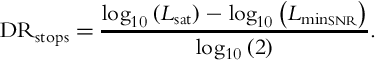
DR is defined as the ratio of luminance of the lightest and darkest elements of a scene or image. In an absolute sense, this ratio can be considered the brightest to darkest pixel, but more commonly it is defined as the ratio of the largest nonsaturating signal to one standard deviation above the camera noise under dark conditions [10, 11]. An equation for DRSNR can be described as the ratio of maximum to minimum input luminance level:
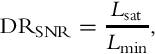
where Lsat is the maximum unclipped input luminance level, defined as 98% of its maximum value (250 of 255 for 24 bit color), and Lmin is the minimum input luminance level for a specified SNR. The ratio can be specified as instantaneous for a single instant of time, or temporal, where the luminance values change over time, that is, light and dark elements over a series of images. Poynton [12] uses the definitions of simultaneous for the instantaneous case, and sequential for the temporal case. The primary focus of this chapter relates to simultaneous measurement, where a single frame of an HDR test chart from a video sequence is analyzed. New classes of imaging sensors are being developed that are capable of directly capturing larger DR on the scale of 5 orders of magnitude (5 log10, 16.6 stops) [13, 14]. For comparison, human vision generally is agreed to have a simultaneous DR capability of approximately four orders of magnitude (4 log10, 13.3 stops) [1, 15], and a sequential DR via adaption of approximately 10 orders of magnitude (10 log10, 33.2 stops) [16, 17].
In order to objectively calculate the capture system DR, an understanding of the imaging and noise transfer function is required. An image sensor measures the radiant power (flux) Φ at each pixel j for each image i. The amount of photons ![]() that are absorbed at each pixel area Aj over time period ti is given by:
that are absorbed at each pixel area Aj over time period ti is given by:
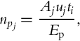
where μj is the mean incident spectral irradiance at pixel j. Ep is the photon energy defined by:

with the wavelength of the photon given by λ, the speed of light c = 2.9979 × 10⁸ m/s, and Planck’s constant h = 6.626 × 10⁻³⁴ Js. Photons incident on the pixel over the exposure time generate an average number of electrons np based on the quantum efficiency of the sensor η(λ):
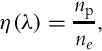
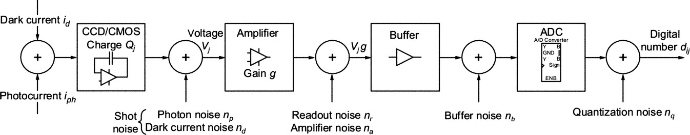
producing a photocurrent iph and photon noise np at each pixel site. Thermally dependent leakage current in the electronics (free electrons in the silicon), known as dark current id contributes to the total charge, as shown in Fig. 1. In conventional current mode, the photocurrent produces a charge Qj on a capacitive integrator generating a voltage Vj amplified with gain g. The voltage gain product Vjg includes readout noise nr and amplifier noise na. Typically, a buffer circuit follows the gain amplifier contributing an additional buffer amplifier noise nb, leading to an analog to digital converter (ADC) with quantization noise nq, resulting in the measured pixel digital number (DN) dij. In linear systems, the DN is proportional to the number of electrons collected with an overall system gain G of units of DN/electrons.
Given a linear transfer model, the noise sources can be summed and we can write an equation for the total system noise at the output of the ADC as:
When specifying noise units, it is understood that the noise magnitude is the RMS value of the random process producing the noise [10]. If npostgain is defined as the sum of the postgain amplifier noise sources nr, na, nb, and nq, the variance is given as:
The variance represents the random noise power of the system, and the standard deviation characterizes the system RMS noise [18]. Finally, Reibel et al. [18] note that no system is strictly linear, and introduce a nonlinear contribution CNL to describe the signal variance that is modeled by a dependence on the total electrons transferred to the sense node capacitor (photoelectrons and dark current electrons) and the overall system gain G resulting in:
A linear transfer model not only permits the summation of noise sources, it also ensures the relative brightness of the scene is maintained. To achieve linearity over the entire sensor, and to minimize fixed pattern noise (including streaking and banding), a radiometric camera calibration is generally required for each pixel, resulting in a total camera response function. The calibrated camera response function can be combined with optical characterization and other camera postprocessing functions such as gamma, tonal response, noise reduction, and sharpening to produce an overall camera opto-electronic conversion function (OECF) [19, 20].
Noise is meaningful in relation to a signal S (i.e., SNR) and can be defined differently depending on how the measurement is performed. If the measurement is concerned with the sensor itself, isolated from the camera postprocessing functions described above, noise can be referenced to the original scene. This can be accomplished by linearizing the data using the inverse OECF, and defining the signal as a pixel difference corresponding to a specified scene density range. Alternatively, if raw data is unavailable or the OECF is unknown (or beyond the scope or measurement capability), or if the focus is on complete system capability (optics, sensor, and camera performance) rather than sensor specific, the signal can be defined with respect to an individual patch pixel level. The evaluation of DR described in this chapter is based on the latter, with a goal of describing a straightforward method that can be used to produce an ever-increasing database of comparable camera system DR measurements. If the variance σsignal2 of the signal is known and the signal is zero mean, the SNR for the minimum input luminance can be expressed as:
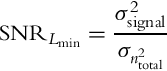
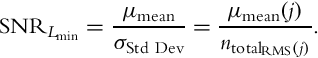
where ![]() is given by Eq. (6). Alternatively, Eq. (8) can be expressed as the ratio of the mean pixel value μmean to the standard deviation σStd Dev, and equivalently to the total RMS noise ntotalRMS(j) as:
is given by Eq. (6). Alternatively, Eq. (8) can be expressed as the ratio of the mean pixel value μmean to the standard deviation σStd Dev, and equivalently to the total RMS noise ntotalRMS(j) as:
Minimum input luminance level is often determined from the density step having a SNR of 1 or greater [11, 21]. The processing software utilized in this study named Imatest [22], performs automatic calculations for ![]() values of 1, 2, 4, and 10. It can be convenient to reevaluate Eq. (9) in terms of stops. Stops is a common photography term where one stop is equivalent to a halving or doubling of light, corresponding more closely to the relative luminance response of human vision [23]. We can express
values of 1, 2, 4, and 10. It can be convenient to reevaluate Eq. (9) in terms of stops. Stops is a common photography term where one stop is equivalent to a halving or doubling of light, corresponding more closely to the relative luminance response of human vision [23]. We can express ![]() in terms of noise in stops by:
in terms of noise in stops by:
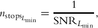
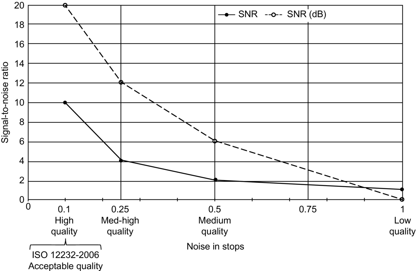
where a ![]() of 1 is equivalent to 1 stop of noise. Fig. 2 illustrates the assignment of the arbitrary quality descriptions (high, medium-high, medium, and low) for 0.1, 0.25, 0.5, and 1 stop of noise as calculated and defined in Imatest, as well as the corresponding SNR values in terms of a luminance ratio as well as in decibels (dB). Finally, DRSNR can also be expressed in terms of relative luminance or stops as:
of 1 is equivalent to 1 stop of noise. Fig. 2 illustrates the assignment of the arbitrary quality descriptions (high, medium-high, medium, and low) for 0.1, 0.25, 0.5, and 1 stop of noise as calculated and defined in Imatest, as well as the corresponding SNR values in terms of a luminance ratio as well as in decibels (dB). Finally, DRSNR can also be expressed in terms of relative luminance or stops as:
The question that remains is: How are the arbitrary quality descriptors chosen and why? We can start to answer this question by reviewing early 1940s era work in human signal detection by Albert Rose, known as the Rose model. The Rose model provided a good approximation of a Bayesian ideal observer, albeit for carefully and narrowly defined conditions [24]. Rose defined a constant k, to be determined experimentally, as the threshold SNR for reliable detection of a signal. The value of k was experimentally estimated by Rose to be in the region of 3–7, based on observations of photographic film and television pictures. Additional experiments using a light spot scanner arrangement resulted in an estimate of k of approximately 5, known as the Rose criterion, stating that a SNR of at least 5 (13.98 dB) is required to distinguish features at 100% certainty. The early empirical determinations of k had several issues. Dependency on a specification of percent chance of detection (i.e., 90%, 50%), included limitations of human vision, such as spatial integration and contrast sensitivity, and included dependence on viewing distance amongst other factors. The development of signal detection theory (SDT) and objective experimental techniques worked to overcome these limitations [25, 26]. For comparison, a binary (yes/no) signal known exactly (SKE) detection experiment, utilizing 50% probability of signal detection and an ideal observer false alarm rate of 1%, resulted in SNRs of 2.3 (7.23 dB) and 3.6 (11.13) for 50% and 90% true-positive rates, respectively [27].
More recently, the ISO 12232-2006 standard defines two “noise based speeds” for low noise exposures that is based on objective correlation to subjective judgements of the acceptability of various noise levels in exposure series images [28]. The two noise based speeds are defined as Snoise40 = 40, (32.04 dB) providing “excellent” quality images, and Snoise10 = 10, (20 dB providing “acceptable” quality images. Examining Fig. 2, a commonality point between the ISO 12232-2006 standard and Imatest occurs at the 20-dB point, pertaining to “acceptable” quality in the ISO standard and “high” quality in Imatest. We note that the ISO standard is based on prints at approximately 70 pixels/cm, at a standard viewing distance of 25 cm. For subjective models utilizing sensor pixels per centimeter values P differing from the ISO standard, an SNR scaling ratio of 70/P is recommended.
Previously reported results for objective calibrated DR test data have yielded limited results and the test methodology used is often unclear. The Cinema5D test website [29] notes “We have at one point in 2014 updated our dynamic range evaluation scale to better represent usable dynamic range among all tested cameras. This does not affect the relation of usable dynamic range between cameras,” however the author does not clearly state what evaluation scale is currently, or was previously, used. In another example, published on the DVInfo website [30], the author describes the minimum input luminance level as “typically, where you consider the noise amplitude to be significant compared to the amplitude of the darkest stop visible above the noise,” but does not further define the term “significant.” Results published on the DxOMark website [31] primarily include still camera and mobile phone tests, implementing a self-designed DR test chart that is limited to 4 density steps (13.3 stops).
2 Method and Materials
2.1 Design
Overall, the procedure for measuring system dynamic range involves four primary steps. Step one includes the setup of the test environment so that overall lighting conditions can be controlled, with reflected light minimized. The ability to set, maintain, and read room temperature is also of importance, as camera noise may be temperature-dependent. The second step is the setup and alignment of the camera under test (CUT) and HDR test chart in order to meet the pixels per patch test requirement. With setup activities complete, the third step includes the collection of sample image frames, followed by postprocessing to create compatible input frames for the analysis software. Finally, step four includes processing of the input frames through the analysis software and the review of data.
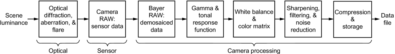
Three main components in the image capture pipeline that should be considered in measurement of DR include the optics, the sensor, and the camera processing workflow [32]. The optics are important in transforming the scene luminance to the image luminance at the sensor, and can reduce the DR as a result of diffraction, aberration, defocus, and flare [33]. The sensor can have limiting factors to DR as well, including saturation on the intensity high end, and noise limitations on the low end [2]. The camera data processing workflow begins with the color transformation (for single sensor systems), generally utilizing a Bayer color pattern followed by a luminance estimate as a weighted sum of the RGB values. Once the data is recorded, further processing may be required based on proprietary codes, log encoding, or other in-camera data manipulation. Care is taken to postprocess the collected data into a standard format for analysis. While the effects on DR of each of the three main components in the image capture pipeline can be analyzed in detail, a goal of this chapter is to focus on complete system capability, as may be used “out of the box.” The measurement and calculation, therefore, includes the combined effects of the optics, sensor, and camera processing as illustrated in the system level model of luminance conversion in Fig. 3.
2.1.1 Test Chart and Processing Software
A DSC Labs Xyla 21 test chart was procured that includes 20 stops of dynamic range via a 21-step, rear-lit, voltage-regulated light source. The Xyla chart, shown in Fig. 4, features a stepped xylophone shape, minimizing flare interference from brighter steps to darker steps. The Xyla chart includes an optional shutter system that allows for the isolation of individual steps in order to reduce the effect of stray light. The use of the shutter system comes at the expense of increased measurement and processing time, as each individual step must be imaged and processed, as opposed to the chart as a whole. The shutter system was not utilized in these experiments due to time constraints; however, the evaluation and characterization of the effect of stray light from the chart itself on the noise measurement is important future work. The Xyla chart is preferred to front-lit reflective charts, as front-lit charts are more difficult to relight evenly over time, as test configurations change or the test environment is altered. Rear-lit, grayscale, stand-alone films require the use of an illuminator, such as a light box, where special care is required to monitor the light source and voltage. The Xyla 21, being an all-enclosed calibrated single unit, simplifies test setup and measurement.
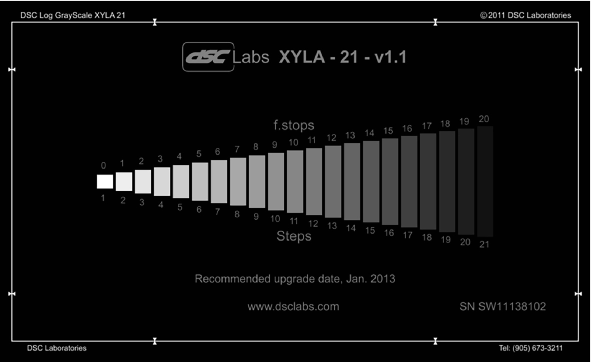
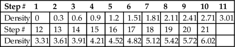
The Xyla-21 chart includes log2 spaced steps, where each linear density step of 0.3 equates to one stop, a doubling (or halving) of luminance. The calibrated density data for the Xyla-21 chart used is provided in Table 1. The calibration is provided by the manufacturer, and the recommended upgrade (recalibration) date is printed on the chart.
Table 1
Xyla-21 density calibration data
| Step # | 1 | 2 | 3 | 4 | 5 | 6 | 7 | 8 | 9 | 10 | 11 |
| Density | 0 | 0.3 | 0.6 | 0.9 | 1.2 | 1.51 | 1.81 | 2.11 | 2.41 | 2.71 | 3.01 |
| Step # | 12 | 13 | 14 | 15 | 16 | 17 | 18 | 19 | 20 | 21 | |
| Density | 3.31 | 3.61 | 3.91 | 4.21 | 4.52 | 4.82 | 5.12 | 5.42 | 5.72 | 6.02 |
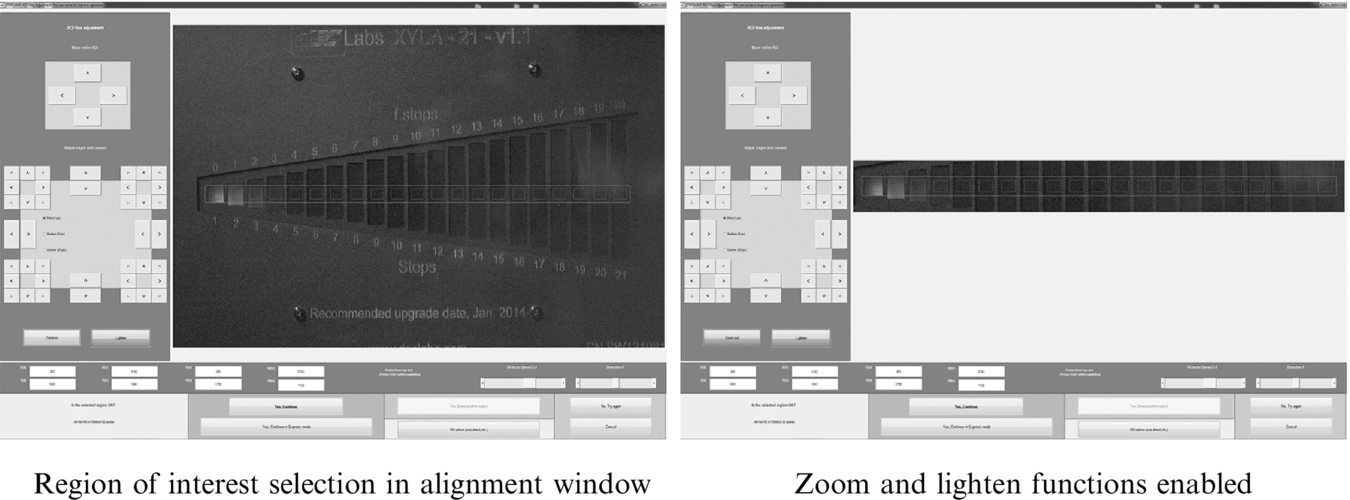
The Stepchart module of the image analysis software Imatest [34] is utilized to process the captured images of the Xyla-21 test chart. The camera distance to the chart is adjusted to maintain approximately 50 pixels per patch horizontal resolution, required by Stepchart [22]. The Stepchart module includes a region of interest (ROI) selection tool that allows for the alignment and selection of ROI for zones as illustrated in Fig. 5. The light gray boxes are the selection region for each individual patch, with software controls allowing adjustment of all patches contained within the red outer box. The right image in Fig. 5 shows the selection tool with zoom and lighten functions turned on, which can be especially helpful when aligning darker zones. A useful alignment hint is to first align the ROIs based on a brightly lit captured frame of the test chart. Imatest will recall this alignment as the default for future images, therefore as long as the camera and chart are not moved, the brightly lit alignment can be used for test frames where the ambient lights have been switched off and darker zones are more difficult to align to. With zone regions selected, Imatest software calculates statistics for each ROI, including the average pixel level and variations via a second-order polynomial fit to the pixel levels inside each ROI. The second-order polynomial fit is subtracted from the pixel levels that will be used for calculating noise (standard deviation), removing the effects of nonuniform illumination appearing as gradual variations.
2.1.2 Selected Cameras
Camera selection was partially based on availability, while best effort was made to include units from various “market” segments. The RED EPIC and ARRI Alexa represent high-end, primarily entertainment industry cameras, both of which claim extended dynamic range. The RED ONE is a very popular entertainment industry camera that continues to find wide use and is available in M and MX models, dependent on the version of the image sensor. The Toshiba and Hitachi cameras represent machine vision cameras that are often used in scientific and engineering applications. The Canon 5D Mark 3 is a latest generation DSLR, and was tested utilizing the manufacturer provided embedded software, as well as open source embedded software known as Magic Lantern [35]. Finally, one of the many new entries into the lower-cost “professional” 4K market cameras, the Black Magic Cinema 4K, was also selected.
2.1.3 Test Procedure
The CUT is mounted on a tripod and placed in a dark test room, kept at an ambient temperature of 23± 2°C, with no light leakage along with the Xyla test chart. Camera lights and all reflective surfaces are masked to prevent reflections off the chart surface. A 25-mm Prime PL mount lens is attached to the CUT utilizing PL type mounts. For large format sensors, in order to maintain the 50 pixels per patch horizontal resolution, a longer focal length lens may be required, such as an 85 mm for the RED Dragon 6K. Cameras with nonPL mounts (such as C, Canon EF) utilize available compatible lenses.
A one-foot straight edge is placed across the front plane of the lens. Measurements are taken at each end of the straight edge to the face of the test chart to ensure the two planes are parallel to an eighth of an inch. The lens aperture is set to full open, and focus is set by temporarily placing a Siemens star on the face of the test chart. Once focus has been verified, the camera is set to the manufacturer recommended native ISO, and data collection begins. The ambient room lights are turned off and the door to the test room is closed, so that only the light from the test chart reaches the CUT. The lens remains at the lowest stop value (wide open) to ensure the luminance of at least the first 2–3 chips will saturate the image sensor at the slowest exposure time (generally 1/24th or 1/30th of a second). A few seconds of video are collected, and then the exposure time is reduced by one-half (one stop). Again a few seconds of video are collected, and the process is repeated for a total of at least 5 measurements to complete the sample collection process. Note that only a short video sequence is required, as only a single frame is used for the simultaneous calculation. Imatest does include a sequential (temporal) noise calculation, where additional frames could be utilized in the difference calculation, but the investigation of this will be future work.
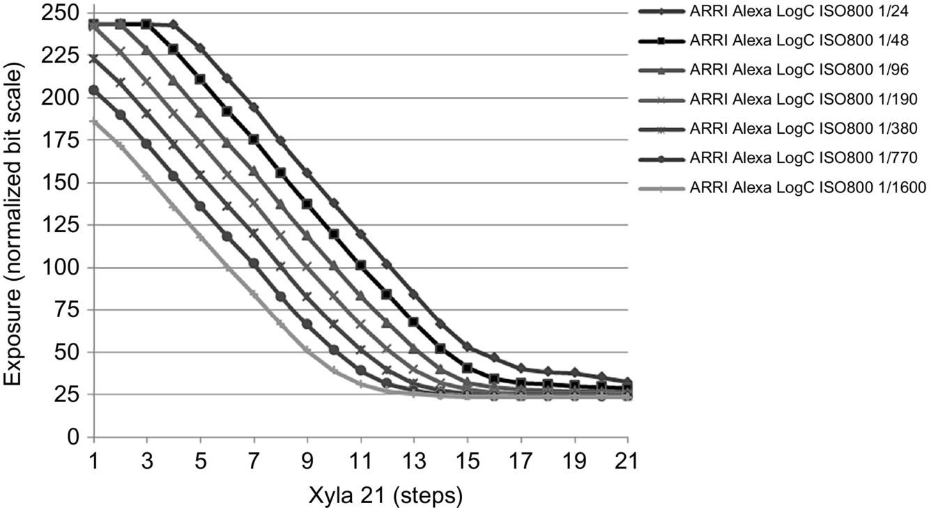
Measured frames are processed through Imatest that can be configured to produce output figures relating to exposure, noise, density response, and/or SNR. A graph of normalized exposure pixel level (normalized to 0–255) is one output that is plotted against the step value of the Xyla21 chart. The original image data, whether 8- or 16-bit pixels, is first conver- ted to quad precision (floating point) and normalized to 1 before any processing is performed. The normalization to 255 is only for the purposes of the output graphical display (historically related to 8-bit file depth and the familiar 255 maximum pixel level). Therefore it is important to note that the full precision of the input file data is utilized in the calculations, independent of the normalized output scale. Sample normalized exposure data for the ARRI Alexa is shown in Fig. 6, noting that seven exposures were collected during this test. The collection of multiple measurements is to ensure an exposure was captured meeting the criteria of the maximum unclipped input luminance level Lsat defined in Imatest as 98% of its maximum value.
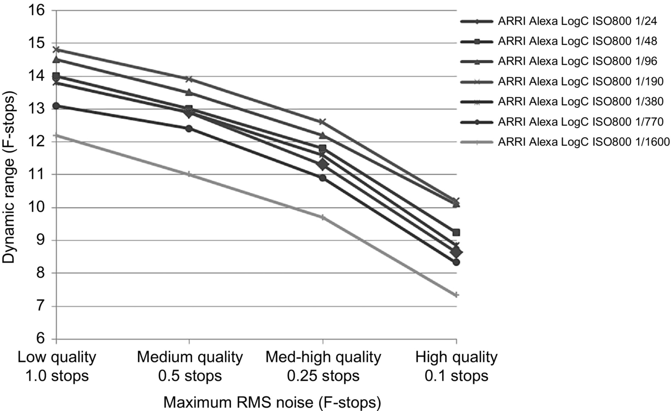
DR is calculated by Imatest, using the minimum luminance step, meeting the maximum RMS noise for each exposure time. This is shown in Fig. 7 for the ARRI Alexa. We can observe the exposure setting that resulted in the peak dynamic range was the one where the brightest chip was just saturated. In the case of the ARRI Alexa data, this was the exposure time setting of 1/190 of a second, resulting in 13.9 stops for a maximum 0.5 stop RMS noise utilized in defining the minimum luminance step.
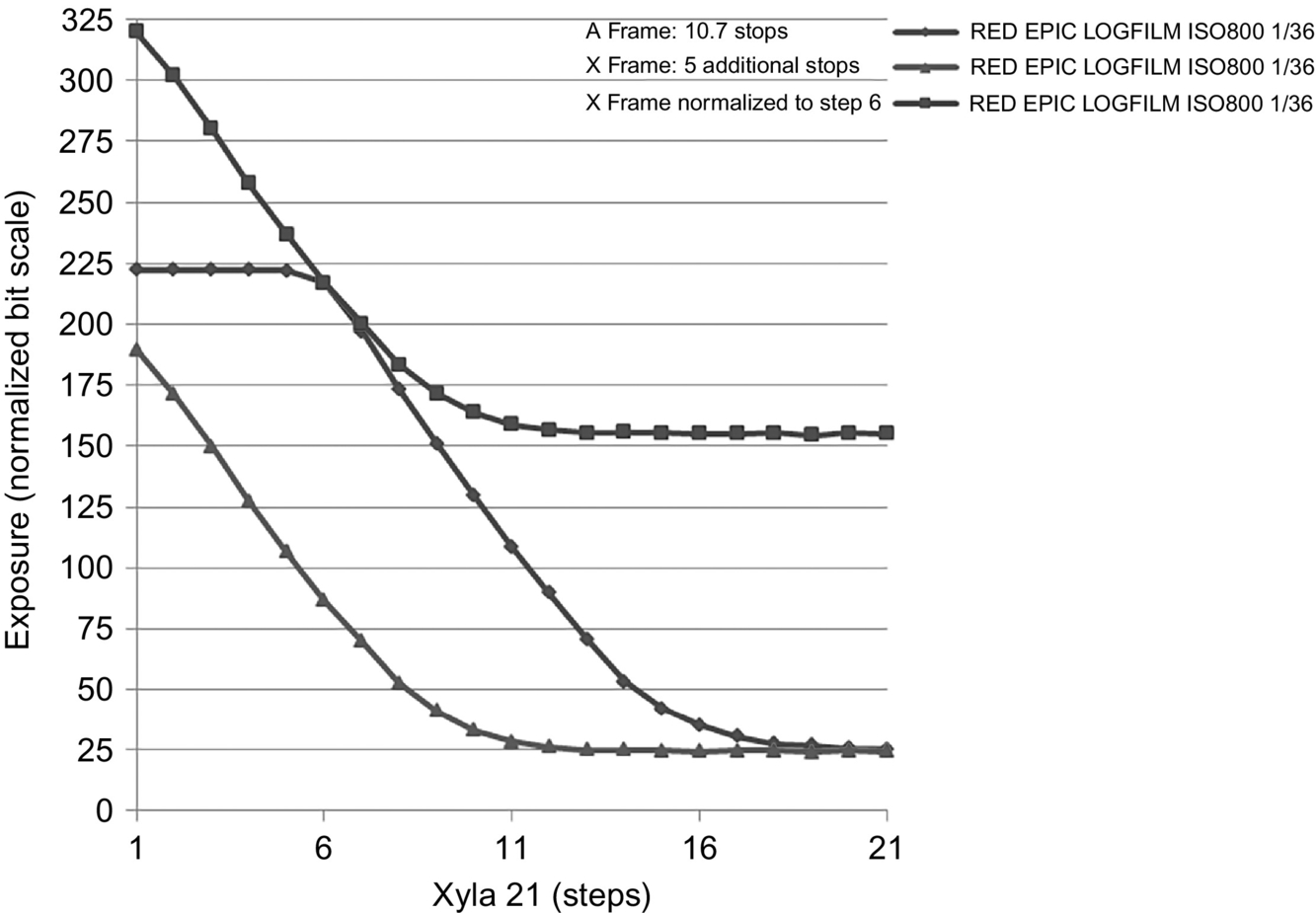
The RED EPIC and DRAGON HDR modes are treated similarly, however, an estimate of the total dynamic range is made based on a combination of both the A and X frames. HDR exposure data for the RED EPIC is shown in Fig. 8, including a “shifted” X frame normalized to the sixth A frame step. Note that for both the RED EPIC and DRAGON, the longest exposure data was utilized to ensure saturation of the A frame, so that more of the X frame is utilized. There may be a limitation in the current setup, where the peak absolute luminance of the Xyla chart is not bright enough to fully extend into the X frame range.
2.1.4 Data Workflow
A significant challenge in testing a large sample of digital imagers is developing data workflows. For as many vendors utilized, there are just as many proprietary data formats, encoding algorithms, export formats, software packages, and postprocessing guidelines. How captured digital data is provided to the user is also manufacturer dependent. For example, ARRI utilizes a dual gain architecture (DGA) with two paths of different amplification for each pixel [36]. ARRI processes the dual path data internal to the camera, providing a single output file, available either as RAW (with external recorder), LogC, or Rec709. ARRI file formats typically use ARRI LUTs for gamma and color space, but are wrapped in standard ProRes422 or ProRes444 wrappers. Generation and application of ARRI specific LUTs for the different outputs is straightforward, resulting in a user-friendly workflow [37].
In some cases, file wrappers, encoding schemes, gamma, and color space functions are vendor-specific, such as with RED Redcode files, but have wide acceptance and are importable and manageable, either through vendor provided software or popular third-party applications [38]. RED provides its HDR digital data as two separate file sequences comprising of A and X frames. Access to both exposure frames has the benefit of increased flexibility in postprocessing, at the cost of increased complexity in understanding the tone-mapping process. The RED software CineXPro includes two tone-mapping functions, Simple Blend and Magic Motion, to assist the user in the tone-mapping process [39].
Manufacturer specific postprocessing workflow and applications used in the creation of sample frames for analysis are summarized in Table 2.
Table 2
System level model of luminance conversion
| Imager | Capture format | Processing steps |
| ARRI Alexa | 12 Bit LogC, ProRes444, 1920×1080 | LogC—Export 16 Bit TIFF from DaVR |
| Rec709—Apply 3D LUT, export 16 Bit TIFF from DaVR | ||
| RED One M/MX | 12 Bit Linear, Redcode36, 4096×2034 | Log/LogFilm Gamma— Apply using CineXPro, export 16 Bit TIFF |
| Gamma3/Color3—Apply using CineXPro, export 16 Bit TIFF | ||
| RED EPIC/DRAGON | 12 Bit Linear, Redcode 8:1, EPIC 4K 16:9, DRAGON 6K 16:9 | LogFilm Gamma—Apply using CineXPro, export 16 Bit TIFF |
| Apply Simple Blend, Magic Motion tone-mapping as required. | ||
| Toshiba HD Hitachi DK | Uncompressed YUV, Blackmagic Hyperdeck Pro Recorder, .MOV wrapper | Rec709 gamma applied by camera. Export 16 Bit TIFF from DaVR |
| BlackMagic | Film Mode, Apple ProRes 422HQ, .MOV wrapper, 3840x2160 | Film gamma applied by camera. Export 16 Bit TIFF from DaVR |
| Canon 5DM3 Magic Lantern RAW Still | ML RAW, Full Frame | Convert ML RAW using RAW2DNG. Export 16 bit TIFF DaVR |
| Canon 5DM3 Magic Lantern HDR Movie | ML H.264, 1920×1080 | Convert H.264 HDR file using AVISynth to HDR JPEG. |
3 Results
Results of imagers tested are shown in Table 3, including the native ISO values used and the Vendor specification when available. The dynamic range measurements are stated in terms of the minimum luminance step meeting the maximum RMS noise, with high, medium-high, medium, and low quality corresponding to 0.1, 0.25, 0.5, and 1.0 stops of RMS noise, respectively. The RED EPIC and DRAGON total measurements are approximate, as it includes the combination of the two measured A and X frames. Data for the RED tone-mapping functions Simple Blend and Magic Motion have been included, as well as measurements for the RED EPIC and DRAGON without utilizing the HDR function.
Table 3
Dynamic range measurement of digital imagers
| Imager—mode, gamma | Stops @ 0.1 RMS noise | Stops @ 0.25 RMS noise | Stops @ 0.5 RMS noise | Stops @ 1.0 RMS noise | Native ISO | Vendor spec. |
| Quality term | High | Medium-high | Medium | Low | ||
| RED DRAGON— HDR x6, Log Film, Total | 7.6 + ∼ 3 | 10.2+∼ 3 | 11.8 + ∼ 3 | 13.1 + ∼ 3 | 250 | 16.5+ |
| RED EPIC—HDR x6, Log Film, Total | 7.6 + ∼ 5 | 9.2 + ∼ 5 | 10.7 + ∼ 5 | 12.0 + ∼ 5 | 800 | < 18 |
| RED EPIC—HDR x6, Log Film, Simple Blend | 11.6 | 13.8 | 15.0 | 16.1 | 800 | N/A |
| ARRI Alexa—Log | 10.2 | 12.6 | 13.9 | 14.8 | 800 | 14.0 |
| RED EPIC—HDR x6, Log Film, Magic Motion | 10.0 | 11.7 | 13.1 | 14.2 | 800 | N/A |
| RED DRAGON—HDR Off, Log Film | 8.4 | 11.1 | 12.4 | 13.6 | 250 | N/A |
| ARRI Alexa—Rec709 | 8.2 | 10.7 | 11.8 | 12.7 | 800 | N/A |
| RED EPIC—HDR Off, Log Film | 8.6 | 10.6 | 11.5 | 12.8 | 800 | 13.5 |
| RED ONE MX—Log Film | 8.8 | 10.4 | 11.5 | 12.7 | 800 | 13.0+ |
| RED ONE MX—Gamma 3 | 8.5 | 10.4 | 11.4 | 12.2 | 800 | 13.0+ |
| Canon 5DM3—Magic Lantern H.264 HDR DUAL ISO 400/1600 | 8.5 | 10.5 | 11.4 | 11.9 | 100 | 14.0 |
| Toshiba IK-HR1S HD—Gamma 0 | 8.5 | 9.5 | 11.1 | 12.0 | 0 dB | N/A |
| Canon 5DM3—RAW Still | 7.6 | 8.8 | 10.6 | 11.6 | 100 | N/A |
| Hitachi DK-H100—Gamma On | 3.9 | 8.3 | 10.6 | 11.2 | − 3a | 10.0+ |
| RED ONE M—Log | 7.7 | 8.9 | 10.4 | 11.7 | 320 | 11.3 |
| RED One M—Gamma 3 | 7.8 | 9.3 | 9.9 | 10.6 | 320 | N/A |
| Hitachi DK-Z50—Gamma On | 5.3 | 7.2 | 9.3 | 10.1 | − 3a | 9.6 |
| Black Magic Cinema 4K—Film | 6.0 | 7.8 | 9.0 | 10.0 | 200 | 12.0 |
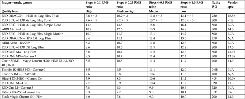
a Hitachi cameras do not specify ISO values for digital gain, instead an arbitrary gain of − 3, 0, or + 3 is available.
In Table 3 results, we attempted to select a “most appropriate” single quality term, and accompanying maximum RMS noise defining the minimum luminance step, that correlates with published data. The table has been arranged from highest to lowest DR, using the Imatest designated “medium” quality. Sorting of the data based on the medium quality term is made after comparison to available Vendor specifications provide where available. The high and medium-high quality results appear to be too stringent to be utilized by most Vendors, especially when marketing for typical applications. Medium quality has relatively close agreement when considering high-end cameras, such as the ARRI Alexa (measured 13.9 stops, specified 14 stops) and industrial cameras, such as Hitachi DK-H100 (measured 10.6 stops, specified 10.0+ stops) and DK-Z50 (measured 9.3 stops, specified 9.6 stops). The case could be made for utilizing the low quality term, as measured data does have close agreement to Vendor specifications in the case of the RED ONE M Log (measured 11.7 stops, specified 11.3 stops), RED ONE MX Log (measured 12.7 stops, specified 13.0+ stops), and Black Magic 4K camera (measured 10.0 stops, specified 12.0 stops). This option seems less than ideal however, as higher noise levels in dark regions are generally undesirable and the low quality term includes a full stop of RMS noise.
4 Discussion
An evaluation of a NROQM to accurately measure and compare the increased dynamic range capability of modern image capture systems is presented. The method utilizes a 21-step, back lit test chart providing luminance patches over a 20-stop range. Data collection, processing, and analysis steps are described as part of an image capture and postprocessing workflow. The workflow requires the use of Vendor software, commercially available postprocessing software, or in some cases, both. Sample data is presented for a number of current generation imaging systems, some of which are extending DR capability beyond traditional digital imaging capabilities.
The image systems tested illustrate the different technologies and implementations available in the market today. In some cases, Vendors utilize a single sensor with single output, relying on the intrinsic capability of the sensor for the maximum DR. In other cases, such as the ARRI Alexa, dual gain sensors are implemented with the Vendor combining, or tone-mapping the dual data sets into a single output, transparent to the end user. Furthermore, with devices such as the RED EPIC and DRAGON, multiple exposures are taken and stored as separate data fields, leaving the tone-mapping as an additional step in the postprocessing workflow. An observation that can be made from testing these various images systems is that when considering DR, it is equally important to consider the postprocessing workflow and how it will be conducted. Manufacturers also offer various gamma functions, which when utilized, result in changes in the final DR.
In real world scenes, quality depends on scene content, such as edges and gradients, as well as target contrast of a signal with respect to the background. Ultimately, we can state that arbitrary quality descriptors are best described as scene dependent. What is deemed “excellent” for one application, or scene, may be “acceptable” for another. Producers of imagery for entertainment may not only allow, but welcome more low light noise to achieve a film like appearance or “look.” Other users, such as in the medical, engineering, or scientific fields, may alternatively require increased signal to noise performance. In other cases, the human eye has been shown to detect well-defined targets when the SNR is less than 0.1 [10]. Manufacturers often add to the confusion by publishing DR or minimum signal level without reference to test conditions or SNR, or without stating if the data is presented for the ideal sensor case, making comparisons difficult. We can state the obvious regarding the definition and application of arbitrary descriptive terms, that they are in fact arbitrary, but can have value and can be compared when they are characterized with respect to a meaningful metric, such as the SNR of the minimum luminance level used to determine DR. The medium quality level pertaining to a 0.5 RMS noise was chosen as a compromise between results that correlate with Vendor supplied data, and a noise level that is undesirable. Medium quality was selected for the general case, however it is open for interpretation for specific use cases. Future work will be conducted in correlating RMS noise based quality evaluation with subjective evaluations.
The results indicate that not all Vendor data correlates with a specific maximum RMS noise defining the minimum luminance step. This may be due to differences in test methodologies, to acceptance of different noise levels, or both. Also of note is the higher end ARRI and RED imaging systems resulted in the greatest DR, however, the RED EPIC and DRAGON results for HDR mode are estimates based on the separate exposure frames. The final realized DR of the RED HDR systems will be a factor of the tone-mapping method employed.
5 Conclusion
As imaging systems continue to develop and evolve, including recent growth in HDR, calibrated measurements of DR that are both transparent and comparable are of increased importance. Manufacturer specifications are often without reference or descriptive narrative as to the computational method. The use of arbitrary quality descriptors may indeed be arbitrary, as what is deemed “excellent” for one application, or scene, may be “acceptable” for another. Value can be added to dynamic range measurement and quality descriptors, and they can be better compared, when characterized with respect to a meaningful metric, such as the maximum RMS noise defining the minimum luminance step used to determine DR. A SNR of 20 dB (0.1 stop of RMS noise) was identified as a reference point having commonality to both ISO Standard 12232-2006 and the test software Imatest. Review of measured results for several modern imaging systems indicate that the industry trend in DR reporting correlates closer with the “medium” quality descriptor in Imatest corresponding to a SNR of 6 dB (0.5 stop of RMS noise when defining the minimum luminance patch), than with the 20 dB metric termed “acceptable” quality in the ISO Standard 12232-2006 and “high” quality in Imatest. The imagers tested have been treated as “systems,” with the combined effect of the optics, the sensor hardware, and the camera processing. Future work will include more specific analysis of the effects on DR based on the contribution of each of the individual sub-systems.