
![]()
PowerPivot Basics
You need one fundamental thing to create stunning visualizations—data. Specifically, you need data in PowerPivot, the Excel add-in that can handle many times the volumes of data that Excel can handle natively—tens of millions of rows if need be. So, to ensure that you are at ease when creating data sets in the Excel Data Model, data sets that are ready for modeling and extending in PowerPivot and for later analysis in Power View, this chapter will take you through the basics of PowerPivot, and will explain how to
- Load data from external sources, specifically SQL Server databases and Excel
- Follow the evolution of changes in the structure of the source data and reflect these modifications in the PowerPivot data set
- Update data in PowerPivot when the source data changes
- Tweak the PowerPivot data set by deleting, renaming, and moving tables and columns
- Select appropriate data types for each column of data
- Apply core formatting to the columns of data
- Sort data
- Filter data
Before we look at these techniques, I need to make one thing extremely clear: PowerPivot is a data repository only. It is not designed to directly modify your source data. All changes (whether they are additions, deletions, or modifications) must be carried out on the source data first. Then the PowerPivot data set will have to be updated with these changes. So although you cannot edit a cell in a PowerPivot table like you can in Excel, you can perform extensive analysis of huge tables of data with near instantaneous response times.
If you already have a working knowledge of PowerPivot then you may not need much, or any, of the information in this chapter. So feel free to cherry-pick the bits that you need, or even to skip ahead to Chapter 10, if you already know how to load data into PowerPivot and apply data types. Perhaps you are using Power Query to load data into the Excel Data Model, in which case you might just want to skim through this chapter to see if there are any interesting complimentary nuggets of knowledge that you may find useful.
Once again, all the sample files used in this chapter are available on the Apress web site. Once downloaded they should be in the folder C:HighImpactDataVisualizationWithPowerBI.
The PowerPivot Environment
PowerPivot exists to store and manipulate large quantities of data. So it follows that getting data into PowerPivot is key, and this is what we will be doing shortly. However, I think that it is best if you first familiarize yourself with the tool itself so that you can feel at home in this new environment.
To start using PowerPivot, you need to follow these steps:
- In Excel, click on the PowerPivot tab. The PowerPivot ribbon will replace the current ribbon.
- Click the Manage button. You will switch to the PowerPivot environment, which is described in Figure 9-1.
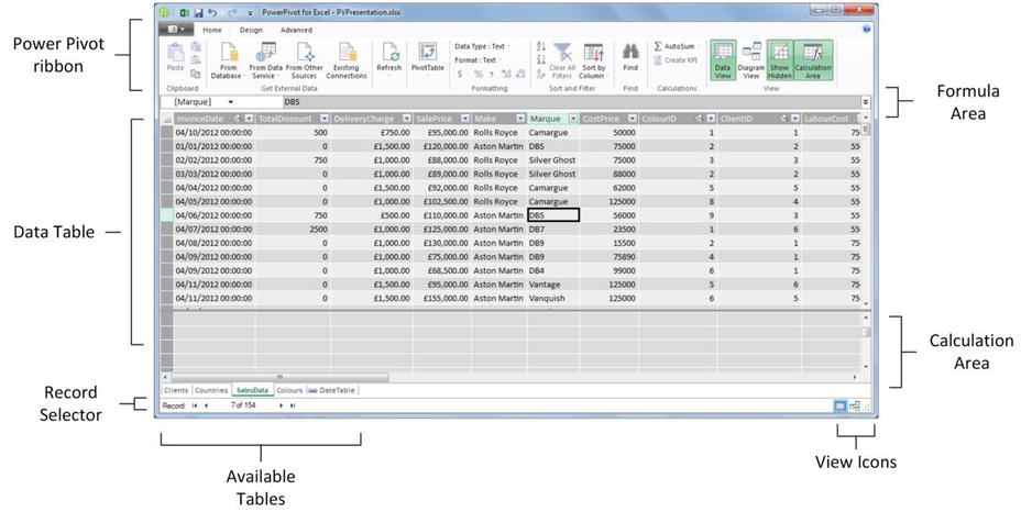
Figure 9-1. The PowerPivot screen
![]() Note This first image contains some data that already exists in PowerPivot. If you have not yet loaded any data, then you will see a very empty screen!
Note This first image contains some data that already exists in PowerPivot. If you have not yet loaded any data, then you will see a very empty screen!
You could well be thinking that this does not look like very much at all yet. However, be reassured, you will soon see what can be done, and exactly how powerful a tool PowerPivot really is. For the moment, it is essential to remember that you have, so to speak, stepped sideways into a separate environment. Although this new world is hosted by Excel (and you can return to Excel instantaneously), it is best if you consider it a kind of parallel universe for the moment. This universe has its own ribbons and buttons and is in a separate window from Excel.
As an aside, we did see, albeit very briefly, the Excel PowerPivot ribbon. We will not be using it any further in this chapter, however. Once PowerPivot is active, you can switch between PowerPivot and Excel just as you normally would flip between open applications. Switching back to an open PowerPivot window is as easy as choosing the PowerPivot window from the available windows.
The PowerPivot Ribbons
So what, exactly, are you looking at when you start PowerPivot? Essentially, you can see three ribbons, which are all devoted to data management:
- The Home ribbon
- The Design ribbon
- The Advanced ribbon
I prefer to explain the PowerPivot ribbons as we start out, as it should make understanding the PowerPivot environment easier. However, if you prefer to skip this section (or possibly use it as reference later), then feel free to jump ahead to the section called “Loading Data into PowerPivot.”
The Home ribbon is used for all core data loading and manipulation such as filtering and sorting. The buttons that it contains are shown in Figure 9-2 and explained in Table 9-1.
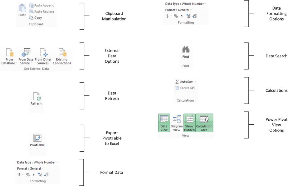
Figure 9-2. Buttons in the Home ribbon
Table 9-1. The Home Ribbon Buttons
|
Button |
Description |
|---|---|
|
Paste |
Lets you paste data that you have just copied to the clipboard (from Excel, for instance) into a new PowerPivot data table. |
|
Paste Append |
Pastes the previously copied data into a table that contains data. The new data is added at the end of the existing data set, which must have been created initially using the Paste command. |
|
Paste Replace |
Pastes the previously copied data into a table that contains data. The new data replaces the existing data set, which must have been created using the Paste command. |
|
Copy |
Copies the selected data so that you can paste it into another application. |
|
From Database |
Starts the process to import data from a Microsoft relational database. |
|
From Data Service |
Starts the process to import data from an online or enterprise data service. |
|
From Other Sources |
Starts the process to import data from one of the other possible sources of data to which PowerPivot can connect. |
|
Existing Connections |
Starts the process to import data using an existing data connection to a data source. |
|
Refresh |
Updates the current PowerPivot data table with the latest version of the data in the data source. |
|
Refresh All |
Updates all the PowerPivot data tables with the latest version of the data from all the data sources that have been used. |
|
PivotTable |
Creates a Pivot Table in Excel using the PowerPivot data set. |
|
Data Type |
Indicates, and lets you alter if it is technically possible, the data type for the current column. |
|
Format |
Indicates, and lets you modify, the format of numerical or date or time data for the current column. |
|
Sort A-Z |
Sorts the data in the current column in ascending (A-Z or 0-9) order. |
|
Sort Z-A |
Sorts the data in the current column in descending (Z-A or 9-0) order. |
|
Clear Sort |
Removes the effects of the sort operation and leaves the data as it was when imported. |
|
Clear All Filters |
Clears all active filters and displays all the data in the table. |
|
Sort By Column |
Allows you to set a column that will provide the sort criteria when you are sorting on the current column in Power View. |
|
Find |
Searches for metadata (column or table names, for example) in the current table. |
|
AutoSum |
Adds a calculated field that aggregates the current column and places the result at the foot of the column. Unless otherwise specified the aggregation is a sum. |
|
Create KPI |
Guides you through the creation process to add a Key Performance Indicator (KPI) to the PowerPivot table. |
|
Data View |
Switches to the view of the data in a table, and tabs of all the tables in the data set. |
|
Diagram View |
Switches to an overview of all the tables and their fields in the data set, with any relationships between the tables. |
|
Show Hidden |
Displays or hides any hidden columns (or other elements) that have been flagged as hidden from client tools. |
|
Calculation Area |
Displays or hides the calculation area under the data table. |
The Design ribbon lets you present the data on screen as well as manage the various properties of the data tables that are joined together. The buttons that it contains are shown in Figure 9-3 and explained in Table 9-2, which follows the image.
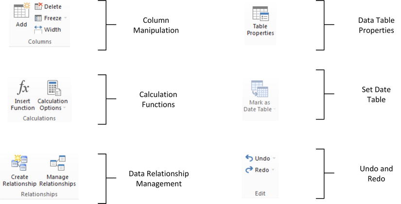
Figure 9-3. Buttons in the Design ribbon
Table 9-2. The Design Ribbon Buttons
|
Button |
Description |
|---|---|
|
Add |
Adds a new column that can contain calculated data. |
|
Delete |
Deletes the selected column and all its data or calculations. |
|
Freeze/Unfreeze |
Uses the selected column as a column of row titles by sliding it to the left of the data table and then leaving it permanently visible. |
|
Width |
Sets the column width in Excel units (based on standard characters in a specific font). |
|
Insert Function |
Jumps to the new column to the right of the data and lists all the available functions you can use to define the required calculation. |
|
Calculation Options |
Lets you choose between automatic and manual recalculation of the functions that you created or forces a manual recalculation. Functions are introduced in Chapter 10. |
|
Create Relationship |
Allows you to define a link, or relationship, between tables. |
|
Manage Relationships |
Allows you to modify or delete relationships between tables. Also lets you add new relationships. |
|
Table Properties |
Lets you modify the columns used or remap them to the source data, as well as filtering the source data when the table is refreshed. |
|
Mark As Date Table |
Defines the table as being a date table that is used for certain specific types of calculation. This is key to using Time Intelligence in PowerPivot. |
|
Undo |
Undoes the last action. |
|
Redo |
Redoes the last action. |
The Advanced ribbon lets you prepare the data for effective visualization in Power View and other tools. It might not, however, be displayed initially in your environment. Nonetheless, it is something that we will need to use eventually to prepare the data set for visualization. So, if it is not displayed,
- Click the File menu to the left of the Home tab.
- Select Switch To Advanced Mode.
The Advanced ribbon will appear to the right of the Design ribbon.
The buttons that it contains are shown in Figure 9-4 and described in Table 9-3.
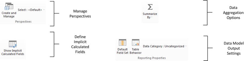
Figure 9-4. Buttons in the Advanced ribbon
Table 9-3. The Advanced Ribbon Buttons
|
Button |
Description |
|---|---|
|
Create And Manage |
Lets you create or modify perspectives (views of the data). |
|
Select: |
Lets you switch between perspectives |
|
Show Implicit Calculated Fields |
Displays implicit calculated fields that are created when you are creating pivot tables and charts |
|
Summarize By |
Lets you select the default autosum function |
|
Default Field Set |
Allows you to define a selection of fields (as well as measures and the order in which they all will appear) that can be added in a single click to Power View. |
|
Table Behavior |
Contains a set of options that you can set to prescribe certain effects in Power View. |
Loading Data into PowerPivot
Ingesting potentially large quantities of data is an inevitable first step when you want to start both analyzing the data and preparing it for display in tools like Power View. In most scenarios you will begin by loading data from one or more sources into the PowerPivot environment. This data can be stored in
- Excel
- A relational database such as SQL Server or Access
- A data warehouse such as SQL Server Analysis Services
- A web resource such as the Azure marketplace
- A text file
Now, although we cannot examine every possible source of data, we will look now at the first two options (SQL Server and Excel) as examples of how to import data into PowerPivot. Once you understand the basics, you will find, I am sure, that adding data from other sources is simply an extension of the core techniques.
If you are going to attempt to analyze large quantities of data, then the data might well be stored in a relational database. After all, for a generation these have been the data repository of choice in corporate environments. So what better place to start our journey with PowerPivot than with Microsoft’s flagship database, SQL Server?
Before ingesting data from SQL Server you will need to know which authentication type is used in your environment. If you are using Integrated Security, then you are probably lucky, since SQL Server should recognize who you are when you attempt to connect to the database. If it does not, then you will need to get a login name and password from your IT department. Finally, it will help if you have an idea about the data that you are looking for. A SQL Server database can contain hundreds of data tables, so once again, having some upfront guidance from your IT staff could save you time.
In this example we will connect to a SQL Server database called CarSalesData and use Integrated Security. If you have installed the sample database under another name, or you are using SQL Server Security (or if you are connecting to your own database), then you will have to take this into consideration when importing your data. If you will be using the sample SQL Server database, then Appendix A explains how to load it into SQL Server.
- In the PowerPivot window, activate the Home tab if this has not already been done.
- Click the From Database button. A popup menu of choices will appear, as shown in Figure 9-5.
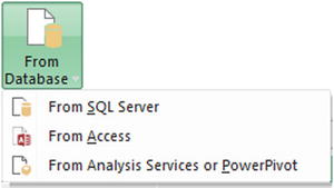
Figure 9-5. Database source menu
- Select From SQL Server. The Table Import Wizard will start up and display the Connect To A Microsoft SQL Server Database pane.
- Enter the Server name, or click on the popup triangle to get a list of available servers. It can take a minute or two to return the list on a large corporate network.
- Choose the authentication type (Integrated Security, in this example). If you are using SQL Server authentication, then enter a user name and password.
- Enter the database name or click on the popup triangle to get a list of available databases on the server. If you are using the sample database, then select CarSalesData. The dialog should look like Figure 9-6.
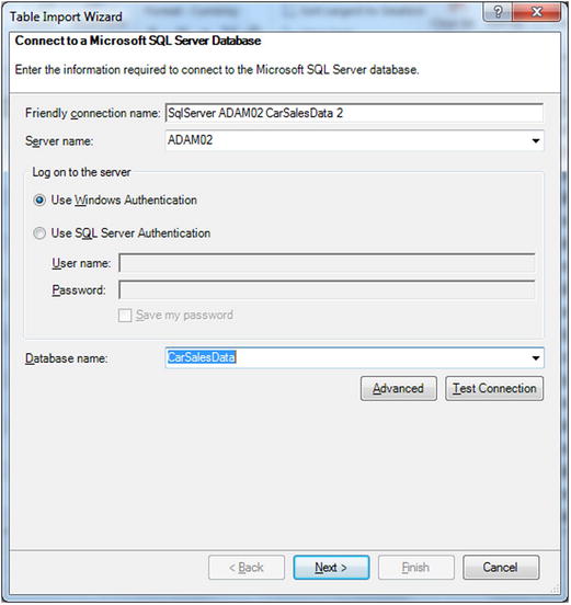
Figure 9-6. The Table Import Wizard
- Click Next. The Choose How To Import Data pane of the Table Import Wizard appears. This is shown in Figure 9-7.
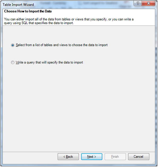
Figure 9-7. The Choose How To Import Data pane of the Table Import Wizard
- Leave Select From A List Of Tables And Views To Choose The Data To Import selected, and click Next. The Select Tables And Views pane of the Table Import Wizard appears.
- Select the following tables (or the tables that interest you if you are using your own data):
- Clients
- Countries
- SalesData
The dialog should look like Figure 9-8.
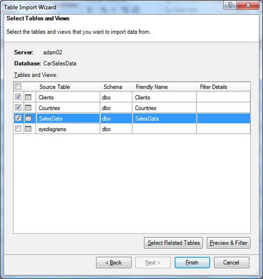
Figure 9-8. The Select Tables And Views pane of the Table Import Wizard
- Click Finish. The tables will be imported into PowerPivot (the dialog will show the import progress), and the Success pane of the Table Import Wizard will be displayed, as shown in Figure 9-9.
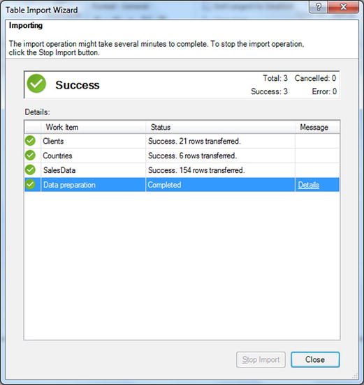
Figure 9-9. The Success pane of the Table Import Wizard
- Click Close The PowerPivot window should now contain data, much like in Figure 9-1 at the start of this chapter. Each table that you chose to import is now a “tab” in PowerPivot.
![]() Note If you chose to select related tables from a database in step 9, then you can click on the Details message in the Success pane of the Table Import Wizard and see the list of all the related tables that were selected, as well as the columns on which they are joined. If the concept of related tables is new to you, then it is explained in greater detail in Chapter 10.
Note If you chose to select related tables from a database in step 9, then you can click on the Details message in the Success pane of the Table Import Wizard and see the list of all the related tables that were selected, as well as the columns on which they are joined. If the concept of related tables is new to you, then it is explained in greater detail in Chapter 10.
When importing data from a database, it can help to have a rough idea of how many records are in each source table. This way you can compare your approximate figure with the number of rows that PowerPivot has succeeded in importing—and you can track the progress of each import to guess how much time remains for each import. If the import fails for some reason, then you may need to review and redo the import process.
Clearly I tried to show you a flawless import process, and I chose something of a “golden path” to successful data import. This meant I had to make sure I did not get distracted and explain too many non-essential options in the Table Import Wizard. However, there are a few options and techniques that it is probably better to know, so we will go through some of them now.
You may not always want to import an entire table from a database. So, at step 9 in the previous section, you have the option in the Select Tables And Views pane of the Table Import Wizard to subset the elements from each table that you want to import. This includes
- The columns that you want to import
- The subset of records that you want to import, filtered by the elements in one or more columns
Here is how you can both take a look at the source data and select the data at source so that only a subset of the source table(s) is imported. Obviously, if you exclude records and columns from the start, then you can invalidate your analyses, so you must filter data with care. However, the smaller the data set is in PowerPivot, the faster you will be able to analyze the data. Not only that, but it will load faster and you will be able to save and load the Excel file faster, too.
- At step (9) in the “Loading Data from SQL Server” section earlier, select the table that you want to subset. It will be highlighted in the wizard.
- Click Preview And Filter. The Preview Selected Table dialog will appear, as shown in Figure 9-10.
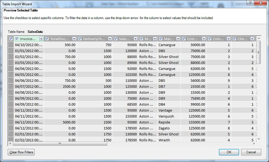
Figure 9-10. The Preview Selected Table dialog of the Table Import Wizard
- Uncheck the columns that you do not want to import. If you cannot see the column titles or data, you can also widen, and narrow, columns by dragging the right column border left or right.
- Click on the filter popup (the downward facing triangle) for each column where you want to apply a selection to the data contained in the column, and check the elements that you want to import. An example of a filter on the Marque (which is another way of saying vehicle model) column is shown in Figure 9-11.
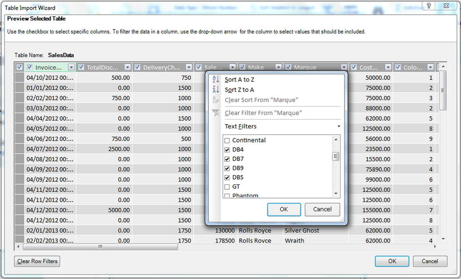
Figure 9-11. Selected car models in the selected table dialog of the Table Import Wizard
- Click OK to return to the Table Import Wizard.
The selected table dialog of the Table Import Wizard also lets you sort the data in the column (in both ascending and descending order) as well as undo a sort operation. If you have applied a complex set of filters you can reset them all by clicking the Clear Row Filters button. Finally, you do not have to accept your filters. You can click the Cancel button and, after confirming that this really is your intention, return to the Table Import Wizard without applying any filters.
The preview and filter options, which are available in the Preview Selected Table pane of the Data Import Wizard, are not limited to merely including or excluding a selection of values from the data source. You can also either define ranges of numeric values to allow into PowerPivot or set the ranges of values that you wish to exclude. Similarly, you can define text ranges to include or exclude.
These options are available in the Text Filters/Number Filters or Date Filters popup that is displayed when you click on the filter popup for a column when importing data. You can see this in Figure 9-12.
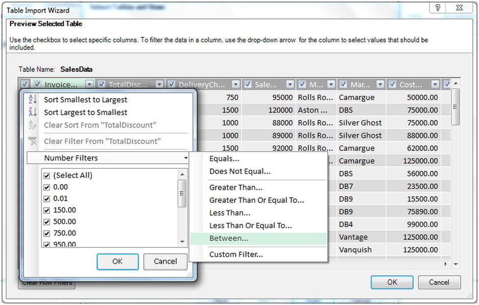
Figure 9-12. Preview and filter options in the selected table dialog of the Table Import Wizard
These options are identical to those that you use when filtering data in PowerPivot itself. As I explain them in the “Filtering Data in PowerPivot Tables” section later in this chapter, I will not explain them here, but I suggest that you skip ahead to this section if you need these options when you are importing data.
![]() Tip You can apply filter options to all the tables that you are importing over the same data source without leaving the Data Import Wizard. Just remember to confirm each preview and filter operation for a table, and then click on the next table that you want to subset. Only when all the filter operations are finished do you close the Wizard.
Tip You can apply filter options to all the tables that you are importing over the same data source without leaving the Data Import Wizard. Just remember to confirm each preview and filter operation for a table, and then click on the next table that you want to subset. Only when all the filter operations are finished do you close the Wizard.
Writing Queries to Select Data
If you have a basic understanding of relational databases—or better, of SQL (the database language used to query SQL Server)—then you can write your own queries to select the data that is imported. A SQL query will select both the rows and the columns of data that will be imported. It can also join tables to select data from several source tables as a single output table.
Fortunately, this does not mean that you have to be a SQL guru to write potentially complex SQL, since the Table Import Wizard has a design pane that will help you create a valid SQL query. Alternatively, if you have existing SQL queries stored as files, you can import them directly to save both time and eventual errors.
To write or design a SQL query that will select the columns and rows of data that you want to use in a PowerPivot table
- At step 8 in the “Loading Data from SQL Server” section earlier, when the Choose How To Import Data pane of the Table Import Wizard is visible, select Write A Query That Will Specify The Data To Import.
- Click Next. The Specify A SQL Query pane of the Table Import Wizard will be displayed.
- If you are a SQL guru, then type or paste in your SQL. If not, then click Design. The Table Import Wizard Design dialog will be displayed (this is explained in more detail in the following pages).
- Expand the table or view containing the fields that you wish to import in the left-hand pane of the dialog.
- Select the fields that interest you. The order in which they are selected will be the column order in the PowerPivot table.
- Click OK. The wizard will write the SQL to filter the data and display it in the dialog. You can then tweak it if you wish.
- Click Finish to import the data.
Finally you may see a few options when using the Table Import Wizard that I have not yet explained. These are outlined in Table 9-4.
Table 9-4. Table Import Wizard Options
|
Option |
Pane |
Description |
|---|---|---|
|
Test Connection |
Connect To A Microsoft SQL Server Database |
Tests that you can connect to the SQL Server instance that you have selected. |
|
Validate |
Specify A SQL Query |
Checks that the SQL is accurate. |
|
Select Related Table |
Select Tables And Views |
Automatically selects any tables that are related (parents or children, for example) to the selected tables. If there are no related tables (or if they are already selected), you will get a message to this effect. |
![]() Tip Writing, or tweaking, a SQL query is a great way to specify the order of columns in a PowerPivot table without having to reorder them manually by dragging them around once the data has been imported.
Tip Writing, or tweaking, a SQL query is a great way to specify the order of columns in a PowerPivot table without having to reorder them manually by dragging them around once the data has been imported.
Filtering Data Using the Table Import Wizard Design Dialog
The Table Import Wizard Design dialog is a surprisingly complete and powerful tool for writing fairly complex SQL that will then be used to import data. Although this dialog is fairly intuitive, it is nonetheless a tool that requires a little explanation if you are to use it efficiently.
The Table Import Wizard Design dialog of the Table Import Wizard contains four main parts:
- The Database View pane (on the left) where you can see all the tables and views that you are authorized to access in the database. You can expand the tables and/or views that you want to use here and select and deselect all the fields you want to import. Remember that if you are using data from more than one table, you will have to specify relationships between all the tables and/or views used.
- The Selected Fields pane (the top pane on the right). This pane lists the fields that you have selected and allows you to
- Change the field order using the up and down icons.
- Remove a field from the list.
- Group and aggregate data.
- The Relationships pane (the middle pane on the right). This pane is hidden by default, and you will need to expand it if you are adding or modifying relationships between tables and/or views. it allows you to
- Detect relationships that already exist in the source database between any of the tables and/or views from which you have selected fields.
- Add new relationships manually by specifying the fields that make up the relationship.
- Delete relationships (in the query that you are creating, not in the source database).
- Change the order of relationships.
- The applied filters pane, which lets you
- Add filters to subset the data.
- Delete filters.
- Modify filters.
These key elements are shown in Figure 9-13.
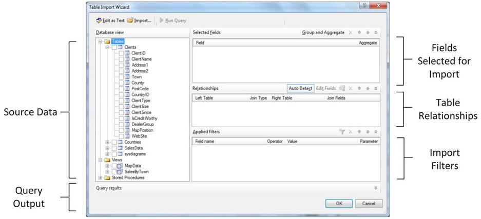
Figure 9-13. The Table Import Wizard Design dialog of the Table Import Wizard
So you can see how the Design dialog can work, I suggest a simple example where we will select data from a few fields in two tables in the source database (Clients and Countries). We will join the tables, and then filter to select data only for car dealers.
- From the PowerPivot screen, choose Existing Connections
 Open Write A Query That Will Specify The Data To Import Next Design. This will display the Design dialog.
 - In the Database View pane (on the left) expand the source tables Clients and Countries.
- Select the ClientName and ClientType fields from the Clients table and select CountryName_EN from the Countries table. You do this by selecting the check box for each required field in the Database View pane. The fields will appear on the right in the upper (Selected Fields) pane.
- Change the field order. In this example I want the Country Name to be just after the Client Name. Consequently you need to click on the CountryName_EN field in the Selected Fields and click on the Move Up arrow.
- Open the Relationships pane by clicking on the Expand Pane icon (the double downward-facing chevron). Click AutoDetect. A new relationship will be added to the Relationships pane. PowerPivot knows that these two tables are linked on the CountryID field in each table.
- Click the Add filter icon (the funnel) above the Applied Filters pane. A new filter will be added showing the first field in the Selected Fields pane.
- Click on the Field name that is shown. A popup of all the available fields in the tables used in the query appears, as shown in Figure 9-14.
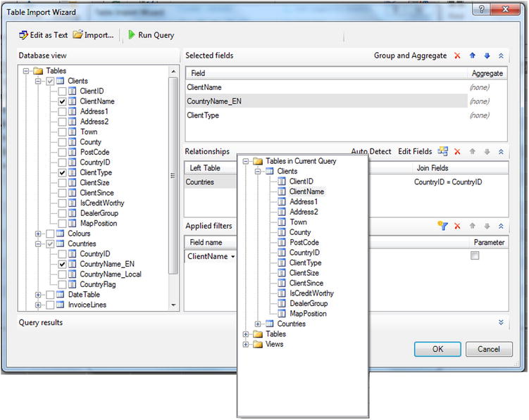
Figure 9-14. Choosing a field to filter on in the Table Import Wizard Design dialog
- Select the ClientSize field.
- Click on the operator in the second column of the filter and select the Is option.
- Click in the third column, enter the text Large and click the tiny plus symbol. The filter will read ClientSize Is Large.
- Click OK. The SQL for the query will be displayed in the wizard.
- Click in the (top) Friendly Name Query box and change the name from Query to something more meaningful, such as ListOfDealers, as shown in Figure 9-15. This will become the table name, saving you from having to rename it later.
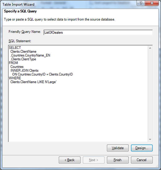
Figure 9-15. The final SQL created by the Table Import Wizard Design dialog
- Click Finish. The query will run and the data will be imported.
There are only a few points to note at this juncture:
- You can create multiple filters. If you do, then all criteria in all the filters will be used simultaneously against the source data to produce (quite possibly) a substantially reduced data set.
- If you choose to define your own relationships between tables, you will need to know which fields to use to create the joins.
- If you are using the Like operator in a filter, then you will need to add a % symbol before and after the text that you are searching for if you want to perform a wildcard search.
- You can always use the designer to create the initial SQL statement and manually tweak it later in the Specify A SQL Query pane of the designer.
List of Tables or Write a Query?
You may be wondering why there are two paths to choose from in the Table Import Wizard in the Choose How To Import The Data pane (which you can see in Figure 9-7 earlier in this chapter). Apart from the reason that we saw immediately in the preceding section—that the Write A Query That Will Specify The Data To Import option allows you to paste in an existing SQL query that you have developed in (say) SQL Server Management Studio—there are other reasons. The differences are outlined in Table 9-5.
Table 9-5. Write a Query or Select from a List of Tables and Views?
|
Option |
Description |
|---|---|
|
Write A Query That Will Specify The Data To Import |
Imports data from multiple tables joined to produce a single output into a single table |
|
Select From A List Of Tables And Views To Choose The Data To Import |
Allows you to select multiple separate tables that are imported into multiple separate tables |
|
Either |
Allow you to select columns |
Importing Other Tables from an Existing Source
Data is nothing if not a moving target, so it is inevitable that you will discover, at times, that you need to import more tables than you originally thought from a data source. This is as easy as the import process that you saw in the previous section, but there is a technique that I want to bring to your attention.
When importing further tables from the same database (or further data from any external source that you are using), reuse the existing connection rather than creating a new one. Now, although you can create a new connection for each source table (even if they are all in the same database), here are some reasons to try to marshal source data so that each table from the same source uses a single, shared connection:
- It makes management of source data much easier when you have dozens of source tables since you can group data by source. This helps you to keep track of the origins of data in your data set.
- It avoids you needing to have dozens of identical connections where only the name changes. This way a single, clearly named connection can replace many others.
- It allows you to refresh all the data from a single source at once if you need to. This is explained in the later section “Data Refresh.”
How then, do you reuse an existing connection to import another data table? Here is how:
- In the Home ribbon click Existing Connections. The Existing Connections dialog will appear.
- Click Open. The Table Import Wizard will start.
You can now add one or more additional tables—either in their entirety or partially—as you did previously. Adding more tables can be done independently of any tables that you have already imported using a given connection. You should, if possible, avoid re-importing tables that are already in the PowerPivot data set. If you import a table twice, PowerPivot will number it Table 1, Table 2, and so on to indicate the duplication. You can always delete duplicate tables as described a little further on in this chapter.
Sometimes column names will change in the source tables from which you have imported data or new columns will be added. Occasionally you will delete columns in an imported table and then want to add them back. Alternatively, you may realize that you no longer need certain columns and want to remove them to save space and declutter the data set. It is also possible that you may have to modify an existing filter on the source data to import more or fewer records. In all of these cases, don’t assume that you have to delete the table in PowerPivot and start over. You can easily modify any link to an existing source table and reimport the data. As an example of this, let’s suppose that you no longer need the InvoiceNumber column in the SalesData table:
- Click inside the SalesData table.
- In the Design ribbon, click the Table Properties button. The Edit Table Properties dialog will be displayed.
- Scroll through the list of columns to the right, until you can see the column that you wish to modify.
- Uncheck the InvoiceNumber column. The Edit Table Properties dialog will look like Figure 9-16.
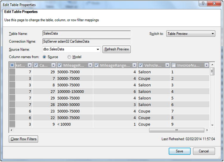
Figure 9-16. The Edit Table Properties dialog
- Click Save. The data will be updated in PowerPivot to reflect the changes you have made to the link to the source data.
This was an extremely simple example of what you can do to tweak the link to source data. As you can imagine, it is far from all that can be done. Some of the techniques that you can apply are described in Table 9-6.
Table 9-6. The Edit Table Properties Dialog Options
|
Option |
Description |
|---|---|
|
Source Name |
Lets you choose a different table or view in the source database to link to the selected PowerPivot table. |
|
Column Names From |
Lets you switch between displaying the columns in the source data or those currently in PowerPivot. |
|
Filter Options |
Clicking on the filter popup allows you to subset source data, as described previously. |
|
Column Check Box |
Lets you add or remove a column from the data link. Removing a column will delete it from the PowerPivot table. |
|
Clear Row Filters |
Removes all filters from all columns. Consequently all the records in the source data will now be imported. |
Loading Data from Excel
There is a fighting chance that some of the data that you want to use in PowerPivot is already in Excel. As long as the data is structured as a list (that is, in tabular form), you can add it to a PowerPivot data set in one of two ways:
- Copy and paste (from any Excel workbook)
- Import (from the Excel workbook that contains the PowerPivot data)
Let’s now look at both of these possibilities to extend the sample data of car sales that you imported earlier from SQL Server.
Copying and Pasting Data from an Excel Workbook
As long as the source data that you wish to add to PowerPivot is not too voluminous (which you will only discover with experience, and which depends, in any case, on the resources of the PC that you are using), you can simply copy and paste data into PowerPivot from Excel like this:
- Go to the Excel worksheet containing the data that you wish to copy. In this example it is the sheet named ReferenceData in the Excel file PowerPivotSample.xlsx.
- Select the data to add to PowerPivot (A1:B10—the table of colors in this example, except for the last line) and copy the table.
- Switch to the Excel workbook in which you are building a PowerPivot data set (if in another workbook) and switch to PowerPivot. Click Paste in the Home ribbon. The Paste Preview dialog will appear.
- Enter a table name (Colours in this example).
- If the data that you copied contains column headers, ensure that the Use First Row As Column Headers. check box is selected. If the data table does not contain column headers, then you can leave this unchecked. The dialog will look like Figure 9-17.
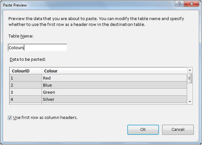
Figure 9-17. Pasting data from Excel
- Click OK.
The data is copied into PowerPivot and becomes a table with the name you entered.
![]() Note You cannot enter a table name that already exists in the PowerPivot data set. If you try this, you will get a warning, and the data cannot be added as a new table.
Note You cannot enter a table name that already exists in the PowerPivot data set. If you try this, you will get a warning, and the data cannot be added as a new table.
If you have copied data from Excel, then the resulting table in PowerPivot is completely static. So if you want to add further data, you need to do it this way:
- In the source file (PowerPivotSample.xlsx if you are following this example) select the data to add (ReferenceData!A11:B11). Copy these cells.
- Switch to PowerPivot, select the Colours table, and click Paste Append in the Home ribbon. The Paste Preview dialog will appear, as shown in Figure 9-18.
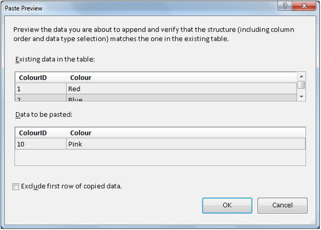
Figure 9-18. The Paste Preview dialog
- Ensure that the format of the copied data is identical to the structure of the destination table, then click OK.
The data that you copied is added to the PowerPivot table at the end of the existing data. If you copied data that includes header rows, then ensure that these do not cause a problem by checking the Exclude First Row Of Copied Data check box.
In some cases it is easier to replace the entire table in PowerPivot with a new table from Excel. In this case you have to
- Select the source data in Excel.
- Switch to PowerPivot and select the destination table.
- Click Paste Replace in the Home ribbon. The Paste Preview dialog will appear, and you must, once again, check that the source and destination formats are identical.
![]() Tip If there is a data type mismatch (that is, if data is perceived as not being compatible), then you will have to correct any anomalies in Excel and attempt the Paste Replace operation again.
Tip If there is a data type mismatch (that is, if data is perceived as not being compatible), then you will have to correct any anomalies in Excel and attempt the Paste Replace operation again.
Importing Data from an Excel Workbook
If you are fortunate enough to have a table of potential source data in the same Excel file as the one where you are creating your PowerPivot data set, then you can import this table directly into PowerPivot without having to copy and paste. Not only is this operation easier to accomplish, but it places less strain on the resources available on the host PC, and it also makes updating and appending data easier.
If you look at the sample file PowerPivotSample.xlsx, you will see a large table of dates in the ReferenceData worksheet. We will now import this table directly into PowerPivot. In case you were wondering, we need a table of dates to apply what PowerPivot calls “Time Intelligence” to our data, but we’ll discuss this more later on in Chapter 10.
- Select the table of data to import in Excel. In this example it is the range E1:Z1462 in the ReferenceData worksheet of the PowerPivotSample.xlsx file.
- Click PowerPivot to activate the PowerPivot ribbon in Excel.
- Click the Add To Data Model button.
The data is added as a new table to PowerPivot. The table is named Table n, but we will see how to change this very shortly.
In the meantime, adding a table from Excel has caused a new ribbon to become visible. This is the Linked Tables ribbon, and its various options (which are shown in Figure 9-19 and describe in Table 9-7) allow you to handle various aspects of linked table data.
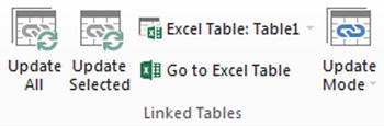
Figure 9-19. Buttons in the Linked Tables ribbon
Table 9-7. The Linked Tables Ribbon Buttons
|
Button |
Description |
|---|---|
|
Update All |
Updates the data in all the PowerPivot tables that are linked to Excel worksheets |
|
Update Selected |
Updates the data in the current PowerPivot table (which is linked to an Excel worksheet) |
|
Excel Table: |
The name of the linked Excel table |
|
Go To Excel Table |
Switches to the table in Excel from PowerPivot |
|
Update Mode |
Lets you set the way in which data is updated (manually or automatically) |
![]() Note You cannot paste data from Excel into a linked PowerPivot table, only into a table that was previously copied into PowerPivot.
Note You cannot paste data from Excel into a linked PowerPivot table, only into a table that was previously copied into PowerPivot.
Excel and SQL Server are, fortunately, not the only places from which you can import data into PowerPivot. You can also source your data from
- Other relational databases
- Dimensional data warehouses
- Web- and cloud-based sources
- File-based sources on your local network
Detailing exactly how you can import data from every available source would take up an entire book. Consequently, I only have space here to list several of the available data sources so that you can see those that are easily accessible. Fortunately the process of importing external data follows a broadly similar model, especially if you are connecting to a database, where the techniques described earlier for SQL Server sources can be applied to a greater or lesser extent.
Data can be imported using one of the three buttons in the Get External Data section of the Home ribbon. The first of these, From Database, is described in Table 9-8.
Table 9-8. Database Sources for PowerPivot
|
Database Data Source |
Description |
|---|---|
|
Access |
Allows you to import data from an MS Access database on your PC or the network |
|
SQL Server |
Connects to a Microsoft SQL Server instance to import data |
|
From Analysis Services or PowerPivot |
Allows you to import data from an SSAS dimensional data store or another PowerPivot data set |
The second button, From Data Service, lets you connect to a web or cloud data source. The options are described in Table 9-9.
Table 9-9. Data Service Data Sources for PowerPivot
|
Data Service Data Source |
Description |
|---|---|
|
From Windows Azure Marketplace |
Connects to the Windows Azure Marketplace to import data from the available data sources |
|
Suggest Related Data |
Attempts to find other useful data sources from the Windows Azure Marketplace |
|
From Odata Data Feed |
Imports data in the Odata format |
The final button, From Other Sources, lets you connect to a wide variety of data sources including many of the most widely used relational databases and file sources. The options are described in Table 9-10.
Table 9-10. Other Data Sources for PowerPivot
|
Data Type |
Description |
|---|---|
|
Microsoft SQL Server |
Connects to a Microsoft SQL Server instance to import data |
|
Microsoft SQL Azure |
Connects to a Microsoft SQL Server Azure database to import data from the cloud |
|
Microsoft SQL Server Parallel Data Warehouse |
Imports data from a Microsoft SQL Server Parallel Data Warehouse appliance |
|
Microsoft Access |
Allows you to import data from an MS Access database on your PC or the network |
|
Oracle |
Connects to an Oracle Server instance to import data |
|
Teradata |
Connects to a Teradata database to import data |
|
Sybase |
Connects to a Sybase database to import data |
|
Informix |
Connects to an Informix database to import data |
|
IBM DB2 |
Connects to a DB2 database to import data |
|
Microsoft Analysis Services |
Allows you to import data from an SSAS dimensional data store |
|
Report |
Imports data from a Microsoft SQL Server Reporting Services report |
|
From Windows Azure Marketplace |
Connects to the Windows Azure Marketplace to import data from the available data sources |
|
Suggest Related Data |
Tries to find related data from the Azure DataMarket |
|
Other Feeds |
Imports data from an atom feed |
|
Excel File |
Allows you to import data from an Excel file on your PC or the network |
|
Text File |
Allows you to import data from a text file database on your PC or the network |
Refreshing Data
Data changes. Nothing is ever permanent, and data less than most things. So just loading your data is rarely the end of the matter. Almost inevitably, you will have to update your data over time as the source data changes.
Now, there is something that we have to be very clear about. PowerPivot is not designed to let you update data in the data set directly. It exists to let you collect and analyze data from disparate sources, but not to modify it. So there is no way in which you can add, alter, or delete data in PowerPivot itself, as you can in Excel. However, if your source data changes, you can refresh the copy of the data that you currently hold in PowerPivot with a couple of clicks. This refresh operation completely replaces the existing data in a PowerPivot table to give you a faithful copy of the latest version of the source data.
PowerPivot is indifferent to the source data type, unless it is a linked Excel worksheet. These have to be refreshed separately. However, all other data sources can be refreshed as a whole, if you so choose.
Refreshing Data from External Data Sources
You can refresh tables that contain data from databases, data warehouses, or web-based data sources in three possible ways:
- For a single table
- For all the tables that were loaded using the same connection (which essentially means those from the same external source)
- For all the tables in a PowerPivot data model
Refreshing a Single Table Connected to an External Data Source
Here is how to refresh a single table. I will use the SalesData table that came from an SQL Server database.
- Select the table whose data you wish to refresh (SalesData, in this example).
- In the Home ribbon, click the Refresh button. The refresh process starts, and the Data Refresh dialog appears as shown in Figure 9-20.
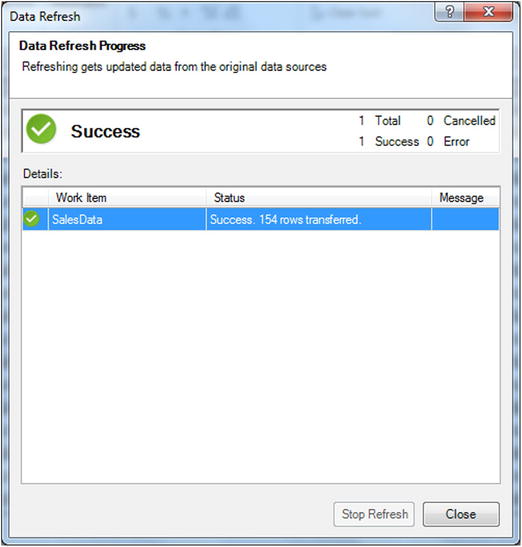
Figure 9-20. The Data Refresh dialog
- Click Close, assuming that the refresh was flagged as successful.
A data refresh will replace all the data in the table with the latest version from the data source. After the refresh operation, the data will, once again, be a copy of the source data that you chose; that is, it will use the selection of columns and any filters that you set up when you loaded the data initially.
![]() Note All refresh operations imply that the structure of the source tables has not been modified. If tables or columns have been renamed or removed, then you will have to tweak the link as described in the earlier section “Modifying Existing Imports.”
Note All refresh operations imply that the structure of the source tables has not been modified. If tables or columns have been renamed or removed, then you will have to tweak the link as described in the earlier section “Modifying Existing Imports.”
Refreshing All the Tables in the Data Set Connected to an External Data Source
This technique is extremely useful when you know that a set of linked tables in an external source has changed, and that consequently they all need to be updated in PowerPivot together for the data to remain coherent and valid. To do this
- In the Home ribbon, click Existing Connections.
- The Existing Connections dialog appears and lists all the current connections to external data sources.
- Click on the connection that you want to update. This is shown in Figure 9-21 using the SQLServer Adam02 CarSalesData connection.
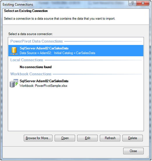
Figure 9-21. The Existing Connections dialog
- Click Refresh. The Data Refresh dialog will appear (as seen previously in Figure 9-20) and the data will be refreshed. If you are dealing with many tables, or large amounts of data, then this could take a few minutes.
- Click Close to close the Data Refresh dialog.
- Click Close to close the Existing Connections dialog.
All the tables where the data originally came from for this data source will be refreshed.
Refreshing All the Tables in the Data Set Connected to an External Data Source
In the case of complex data sets or outdated data, you may well have no choice but to refresh all the tables at once. To do this
- In the Home ribbon, click the popup menu for the Refresh button and select Refresh All.
- The Data Refresh dialog appears and lists all the tables whose data is being updated from the data sources.
Refreshing Data from Linked Excel Worksheets
If you have data that you linked to(but have not copied and pasted) from Excel, then you can also update the data either table-by-table or all the tables together.
Refreshing a Single Table Connected to an Excel Worksheet
Here is how to refresh a single table connected to an excel worksheet:
- Select the table whose data you wish to refresh (DateTable in this example).
- Ensure that the Linked Table ribbon is activated.
- Click the Update Selected button.
The data will be refreshed from the source worksheet. Here, too, the current PowerPivot data will be replaced by the data in the source.
Refreshing All the Tables in the Data Set Connected to Excel Worksheets
In the case of complex data sets or outdated data you may well have no choice but to refresh all the tables at once. To do this
- Click inside any table that is linked to Excel data (remember that there is a tiny chain icon to the left of the table name to indicate that this is a linked Excel table).
- Ensure that the Linked Table ribbon is activated.
- Click the Update All button.
![]() Note Data that has been copied and pasted from Excel into PowerPivot cannot be updated. You have to copy and replace the data as described previously.
Note Data that has been copied and pasted from Excel into PowerPivot cannot be updated. You have to copy and replace the data as described previously.
In a complex data set you could end up with dozens of connections. Managing these connections, and deleting unused connections, can help you stay on top of your data. So, if you need to delete a connection
- Delete all the tables that were imported using this connection.
Deleting all the tables for a connection will remove the connection.
![]() Note If you want to see which tables are based on an existing connection, just try and delete the connection by clicking the Delete button in the Existing Connections dialog. A warning dialog will appear telling you which are the tables that you have to delete to remove the connection.
Note If you want to see which tables are based on an existing connection, just try and delete the connection by clicking the Delete button in the Existing Connections dialog. A warning dialog will appear telling you which are the tables that you have to delete to remove the connection.
When you are importing data from an external source, PowerPivot will try and convert it to one of the six data types that it uses. These data types are described in Table 9-11.
Table 9-11. PowerPivot Data Types
|
Data Type |
Description |
|---|---|
|
Date |
Stores the data as a date and time in the format of the host computer. Only dates on or after the 1st of January 1900 are valid. |
|
True/False |
Stores the data as Boolean—true or false. |
|
Text |
Stores the data as a Unicode string of 536,870,912 bytes at most. |
|
Whole Number |
Stores the data as integers that can be positive or negative but are whole numbers between9,223,372,036,854,775,808 (-2^63) and 9,223,372,036,854,775,807 (2^63-1). |
|
Decimal Number |
Stores the data as a real number with a maximum of 15 significant decimal digits. Negative values range from -1.79E +308 to -2.23E -308. Positive values range from 2.23E -308 to 1.79E + 308. |
|
Currency |
Stores the data as currency—that is, from -922,337,203,685,477.5808 to 922,337,203,685,477.5807 with four fixed precision decimal digits. |
For a column of data to be imported successfully, all the data in the column must be of the required data type. If any column cannot be converted to the chosen data type, the column will default to text.
Once data has been imported into PowerPivot you can, in certain cases, change the data type. You can, however, only change to a more wide-ranging data type. That is, you can convert most data to text, but alphabetical text cannot be converted to numbers, for instance.
If you are importing data from a relational database, there is a very strong chance that the source data type will map fairly easily to a corresponding PowerPivot data type. So a numeric column will remain as one of the numeric types, and therefore you will be able to aggregate it in PowerPivot. However, other less strongly typed sources (and specifically Excel) can be trickier. It only takes one text field in a million records for the whole column to become a text field in PowerPivot. If this happens, then you cannot force a data type change after the import has finished. You will have to delete the imported table and clean up the source data before re-importing it.
If the data needs any form of cleansing or rationalization then you could be better advised to use Power Query to import int into the Excel data model. This is described in Chapters 12 and 13.
Assuming that all has gone well, you now have a series of tables from various sources successfully added to your PowerPivot data set. You can see these data tables as tabs in the PowerPivot window, much like you see Excel worksheets in an Excel workbook file. It will soon be time to see what we can do with this data, but first, to complete the roundup of overall data management, you need to know how to do a few things like
- Rename tables
- Delete tables
- Move tables
- Move around a table
- Rename a column
- Delete columns
- Move columns
- Set column width
- Freeze columns (set row titles)
Let’s begin by seeing how you can tweak the tables that you have imported.
Suppose that you wish to rename a table, such as the table of dates that you imported from Excel earlier. These are the steps to follow:
- Right-Click on the table name tab at the bottom of the PowerPivot window.
- Select Rename. The current name will be highlighted in the tab.
- Enter the new name, or modify the existing name.
- Press Enter.
Deleting a table is virtually identical to the process of renaming one—you just right-click on the table name tab and select Delete instead of Rename. As this is a potentially far-reaching operation, PowerPivot will demand confirmation.
Moving a table is virtually identical to the way in which you move worksheets in an Excel workbook (a process that I am sure that you already know by heart).
- Click on the table name at the bottom of the PowerPivot window.
- Drag the table left or right to its new position.
A small black triangle indicates where the table will move. This is shown in Figure 9-22.
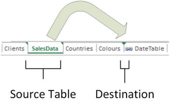
Figure 9-22. Moving a table
![]() Note Moving a table is something that you are likely to do only because it makes it easier for you to traverse the collection of tables that make up a data set. It will have no effect on the data itself or the way in which PowerPivot uses this data.
Note Moving a table is something that you are likely to do only because it makes it easier for you to traverse the collection of tables that make up a data set. It will have no effect on the data itself or the way in which PowerPivot uses this data.
The other core table management options are described in Table 9-12.
Table 9-12. Essential Table Manipulation Options
|
Table Option |
Description |
|---|---|
|
Delete |
Removes the table, its data, and any calculated fields from the PowerPivot data set. |
|
Rename |
Renames the table in PowerPivot. |
|
Move |
Moves the table relative to the other table tabs. |
|
Description |
Lets you add a description to the table that can be used by Power View (and potentially other client tools). |
|
Hide From Client Tools |
Leaves the table in Power View, but makes it invisible to Power View (and any other client tools). |
|
Show Calculation Area |
Displays the table calculation area under the table data. There is more on this in Chapter 10. |
Using the scrollbars to move around a table is one very easy way to look at your data. However, if you have very large tables that contain dozens or hundreds of columns, then it can be easy to spend an excessive amount of time sliding around the data in search of a specific column.
To mitigate the difficulty, PowerPivot lets you
- Select a column name to move to from a list of available columns
- Search for a column
Given the usefulness of these options, it is well worth a rapid detour to see how you can use them.
Selecting a Column from the List of Available Column Names
If you want to leap straight to a column of data (and presuming you know which column contains the data that interests you), all you have to do is
- Click on the popup (the downward-facing triangle) for the Field List (on the left, immediately above the table grid). An alphabetical list of the fields in the table appears, as shown in Figure 9-23.
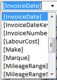
Figure 9-23. The list of columns in a table
- Click on the name of the field that contains the data that you want to study.
The cursor will jump to the chosen column in the table. The cursor will remain on the same record it was on before you selected this column.
In the case where you have a pretty good idea of the column name (or table name) that you are looking for, you can get PowerPivot to locate it for you.
- In the Home ribbon, click Find. The Find Metadata dialog will be displayed.
- Enter all or part of the field name that you want to locate. I suggest entering the word InvoiceDate (without quotes) if you are using the sample data. The dialog will look like Figure 9-24.
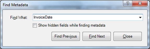
Figure 9-24. The Find Metadata dialog
- Click Find Next (or Find Previous) until you have located the table and/or column that you are looking for.
- Click Close.
In this example I was looking for column titles, but you can look for any element that PowerPivot contains, whether it is a table, a column, a KPI, or a hierarchy (these latter two are explained in Chapter 11), for instance. Also, if the element is hidden (more of this in the next chapter) you can check the Show Hidden Fields While Finding Metadata check box to have PowerPivot look for hidden elements too.
Also—even if I did mention it in passing in step 2—it is worth noting that you do not have to enter the complete title of a field (or any other valid metadata item). Part of the name will suffice.
![]() Note The Find Metadata dialog will remember the last few searches. So if you are reusing a previous search, you do not have to type the search element in a second time—you can select it from the popup list that appears if you click the popup menu triangle at the right of the search box.
Note The Find Metadata dialog will remember the last few searches. So if you are reusing a previous search, you do not have to type the search element in a second time—you can select it from the popup list that appears if you click the popup menu triangle at the right of the search box.
Now let’s see how to perform similar actions—but this time inside a table—to the columns of data that make up the table.
Renaming a column is pretty straightforward. All you have to do is
- Right-click on the title of the column that you wish to rename. In this case it will be CountryName_EN. The column will be selected and the context menu will appear. This is shown in Figure 9-25.
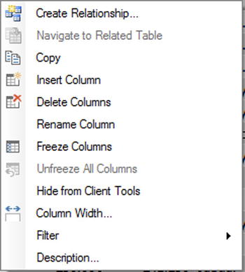
Figure 9-25. The PowerPivot context menu
- Select Rename Column from the context menu. The current column name will be highlighted.
- Type in the new name for the column (CountryName) and press Enter.
And that is it; your column has been renamed. You cannot, however, use the name of an existing column in the same table. If you try, PowerPivot will name the column InvoiceDate2, for example.
Although renaming a column may seem trivial, it can be important. Consider other users first; they need columns to have instantly understandable names that mean something to them. Then there is the Power BI Q&A natural language feature. This will only work well if your columns have the sort of names that are used in the queries—or ones that are recognizable synonyms. Finally, you cannot rename columns in Power View, so you really need to give your columns the names that you are happy seeing in the final output.
![]() Note Although renaming a column is a piece of cake, the consequences of performing this action can be far-reaching. This could mean that any calculated columns or calculations that refer to this column will now not work (you will see how to create these in the next chapter). Also any visualizations that you have already created that use this column, whether it is using Excel or Power View, will now not work properly. So you should really try and get all your data set elements correctly named before you proceed to create calculations and visualizations.
Note Although renaming a column is a piece of cake, the consequences of performing this action can be far-reaching. This could mean that any calculated columns or calculations that refer to this column will now not work (you will see how to create these in the next chapter). Also any visualizations that you have already created that use this column, whether it is using Excel or Power View, will now not work properly. So you should really try and get all your data set elements correctly named before you proceed to create calculations and visualizations.
Deleting a column is equally easy. You will probably find yourself doing this when you have either brought in a column that you did not mean to import, or you find that you no longer need a column. So, to delete a column
- Right-click on the title of the column that you wish to delete. The column will be selected and the context menu will appear.
- Select Delete Columns from the context menu. Unless the column is empty, the confirmation dialog will appear as shown in Figure 9-26.
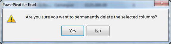
Figure 9-26. Deleting a column
- Click OK. The column will be deleted from the table.
Deleting unused columns is good practice, as this way you will
- Reduce the memory required for the data set.
- Speed up use of the data in tools like Power View.
- Reduce the size of the Excel file.
![]() Tip Deleting a column really is permanent. You cannot use the undo function to recover it. Indeed, refreshing the data will not add the column back into the table either. If you have deleted a column by accident, you can choose to close the Excel file without saving and reopen it, thus reverting to the previous version. Otherwise you can tweak the link to the source data and add the column name, as described a few pages previously.
Tip Deleting a column really is permanent. You cannot use the undo function to recover it. Indeed, refreshing the data will not add the column back into the table either. If you have deleted a column by accident, you can choose to close the Excel file without saving and reopen it, thus reverting to the previous version. Otherwise you can tweak the link to the source data and add the column name, as described a few pages previously.
When you first load data from Excel or SQL Server in this chapter (or from the sources that you are using in your work with PowerPivot) you will noticed that the structure of the tables in PowerPivot reflects exactly the structure of the source tables. All columns appear in PowerPivot in the order in which they appear in the source. Now, as we saw earlier, if you are specifying the data to load using a query or the Table Import Wizard Design dialog, then you can set the order of the columns as you want them in PowerPivot. However, if you prefer to work faster and import a group of tables at once, you have to accept the table structure as is.
However, all is not lost if you want to reorganize the column structure. Doing this can be useful from a data analysis perspective, since it allows you to place columns in an order that makes sense to you. So suppose that you want to move the CostPrice column to the left so that it is now beside, and to the right, of the SalePrice column. This is what you have to do:
- Click on the column you wish to move (CostPrice). The column will be selected. Ensure that you release the mouse button.
- Move the mouse pointer over the column title. The cursor becomes a four-headed arrow.
- Drag the column left or right to its new position. A slim vertical bar will appear to indicate where the column will be moved between existing columns, and you will see a “shadow” of the column header under the mouse pointer.
Figure 9-27 shows how this is done.
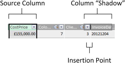
Figure 9-27. Moving a column
One final thing that you may want to do to make your data more readable—and consequently easier to manipulate—is to adjust the column width. I realize that as an Excel user you may find this old hat, but in the interests of completeness, here is how you do it:
- Place the mouse pointer over the right-hand limit of the column title in the column whose width you want to alter. The cursor will become a two-headed arrow.
- Drag the cursor left or right.
As is the case with Excel, you can select several adjacent columns before widening (or narrowing) one of them to set them all to the width of the column that you are adjusting. You can also double-click on the right-hand limit of the column title in the column whose width you want to alter to have PowerPivot set the width to that of the longest element in the column. Finally you can right-click on a column title and select Column Width. . . to display the Column Width dialog and set the width exactly.
When taking an in-depth look at your data you are likely to want to set row titles to the left of the window, just as PowerPivot sets the column titles at the top of the data. There are essentially two ways to do this, depending on whether you wish to use a single column as the row titles or a group of columns.
If all you want to do is to use a single column for the fixed row titles, then all you have to do is
- Right-click on the title of the column that you wish to use. The column will be selected and the context menu will appear.
- Select Freeze Columns from the context menu and the selected column will be moved to the left of the table and its contents will be fixed as row titles.
You can now scroll right in the PowerPivot window, and the leftmost column will always remain visible. You will see a slightly thicker column border to the right of the frozen column as a visual indication that the row titles have been set.
If you want to use several columns as row titles
- Move the columns that you wish to use to the left of the PowerPivot window as a contiguous block.
- Select the titles of these columns.
- Right-click on the title of one of the columns and choose Freeze Columns.
You can now scroll right in the PowerPivot window and the chosen columns will always remain visible.
![]() Note If you prefer not to use the context (right-click) menu, then the width, freeze, and delete options are also available in the Design ribbon.
Note If you prefer not to use the context (right-click) menu, then the width, freeze, and delete options are also available in the Design ribbon.
To unfreeze all the row titles all you have to do is right-click on any column title—whether it is a frozen row title or an ordinary column—and select Unfreeze All Columns.
PowerPivot allows you to apply basic formatting to the data in the tables that it contains. You need to remember, however, that a PowerPivot table is meant to be raw data, and that you should probably not be using this data directly for presentation purposes. After all, that is what Power View is for. However, if you format the data in PowerPivot, then it will appear using the format that you applied in most presentation tools (including Power View). So it is probably worth learning to format data for a couple of reasons:
- You can save time and multiple repetitive operations when creating reports and presentations by defining a format once in PowerPivot. The data will then appear using the format that you applied in multiple visualizations using many different tools.
- It can help you understand your data more intuitively if you can see the figures in a format that has intrinsic meaning.
Here is how to format a column (of figures in this example):
- Assuming that you have the PowerPivot window open, click on the tab that contains the table where you wish to format data.
- Click inside the column that you want to format (CostPrice in the sample file).
- In the Home ribbon, click on the Thousands Separator icon (the comma in the Formatting section). All the figures in the column will be formatted with a thousands separator and two decimals.
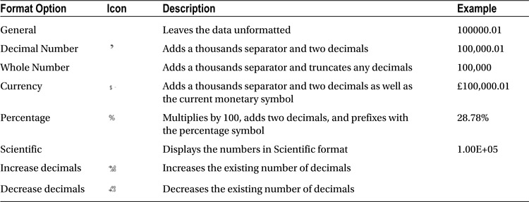
The various formatting options available are described in Table 9-13.
Table 9-13. Currency Format Options
If you wish to return to “plain vanilla” data, then you can do this by selecting the General format. Remember that you are not in Excel, and you cannot format only a range of figures—it is the whole column or nothing. Also there is no way to format nonadjacent columns by Ctrl-clicking to perform a noncontiguous selection. Fortunately you can select multiple adjacent columns, and you can format them in a single operation if, and only if, all the columns are the same data type. Be warned, however, that “same data type” means precisely that. So if one column is a whole number and the one beside it is a decimal, they are considered to be different data types.
![]() Note Numeric formats are not available for selection if the data in a field is of text or data/time data type.
Note Numeric formats are not available for selection if the data in a field is of text or data/time data type.
Other Currency Formats
By default PowerPivot will apply the currency format that has been set for the PC as a default. If you wish to use another format, then you can do it in this way:
- Click on the popup (the downward-facing triangle) to the right of the currency format icon. This will display a list of available formats.
- Select the currency symbol that you want, or click on More Formats to display all the available currency formats, as shown in Figure 9-28, then click OK.
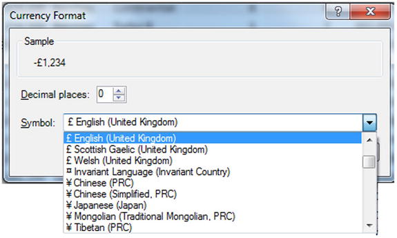
Figure 9-28. The currency format dialog
![]() Note The thousands separator that is applied, as well as the decimal separator, will depend on the settings of the PC on which the formatting is applied.
Note The thousands separator that is applied, as well as the decimal separator, will depend on the settings of the PC on which the formatting is applied.
Manipulating Data in PowerPivot
Assuming that all has gone well, you now have a set of data tables loaded into PowerPivot, and you have formatted them to suit your taste. The next thing that you may want to do is to take an initial look at the data and see what it contains. PowerPivot contains a set of core functions that are there to help you in this, and that specifically allow you to
- Sort data in PowerPivot tables
- Filter data in PowerPivot tables
Both of these techniques should help you take a first look at your data; let’s see how they can be applied.
Sorting Data in PowerPivot Tables
A PowerPivot table could contain millions of rows, so the last thing that you want to have to do is to scroll down through a random data set. Fortunately ordering data in a table is simple:
- Click inside the column you want to order the data by. I will choose the Make column in the SalesData table.
- Click the Sort A-Z icon in the Home ribbon to sort it in ascending (alphabetical) order.
The table will be sorted using the selected column as the sort key, and even a large data set will appear correctly ordered in a very short time. If you want to sort a table in descending (reverse alphabetical or largest to smallest order) order, then click on the Sort Z-A icon.
![]() Tip If you need a visual indication that a column is sorted, look at the popup icon (the downward-facing triangle) to the right of the column name. You will see a small arrow that faces upward to indicate a descending sort or downward to indicate an ascending sort.
Tip If you need a visual indication that a column is sorted, look at the popup icon (the downward-facing triangle) to the right of the column name. You will see a small arrow that faces upward to indicate a descending sort or downward to indicate an ascending sort.
PowerPivot alters the text in the sort icon slightly depending on the data type of the column in which you have clicked. This makes the result even more comprehensible, if anything.
- For a numeric column, the icons read Sort Smallest To Largest and Sort Largest To Smallest.
- For a date column, the icons read Sort Oldest To Newest and Sort Newest To Oldest.
If you want to remove the sort operation that you applied and return to the initial data set as it was imported, all you have to do is click the Clear Sort icon in the Home ribbon.
![]() Note You cannot perform complex sort operations; that is, you cannot sort first on one column, then—carry out a secondary sort in another column (if there are identical elements in the first column), as you can in Excel. You also cannot perform multiple sort operations sorting on the least important column and then progressing up to the most important column to sort on to get the effect of a complex sort. This is because PowerPivot always sorts the data based on the data set as it was initially loaded.
Note You cannot perform complex sort operations; that is, you cannot sort first on one column, then—carry out a secondary sort in another column (if there are identical elements in the first column), as you can in Excel. You also cannot perform multiple sort operations sorting on the least important column and then progressing up to the most important column to sort on to get the effect of a complex sort. This is because PowerPivot always sorts the data based on the data set as it was initially loaded.
Filtering Data in PowerPivot Tables
If you are dealing with millions of rows, then you will probably want to subset the data so that you can take a look at a less overwhelming amount of information. This is where PowerPivot’s filtering capabilities can really help you. Suppose that you only want to see the data for a certain make of car in the SalesData table.
- Click inside the column that you will be using as a basis for filtering the data in the table.
- Click on the popup icon (the downward-facing triangle) to the right of the column name. The Filter popup will appear, as shown in Figure 9-29, where I want to filter the VehicleType column.
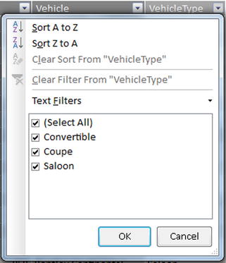
Figure 9-29. The Filter popup
- Uncheck all the boxes for elements that you wish to remove from the filtered data subset.
- Click OK.
The table will be filtered so that it only displays records that match the filter criteria. You will have a couple of visual indications that a filter is active:
- The popup icon to the right of the column name now contains a small funnel image.
- The row count indicator at the bottom left of the PowerPivot window has changed to show the number of filtered records.
You can filter as many columns as you wish at any one time. Each filter will complement any existing filters and further reduce the amount of visible data. If you want to know quickly what constitutes an active filter, all you have to do is to hover the mouse pointer over the popup icon and a small window will appear displaying the filter settings. An example of this is shown in Figure 9-30.
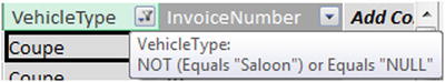
Figure 9-30. The Filter popup
![]() Tip If you want to filter quickly on just one data element—for instance, if you want to display only the Aston Martin make—then PowerPivot has a slick way of letting you do this. Simply right-click in the requisite column (Make), click on the required manufacturer name (Aston Martin), and select Filter
Tip If you want to filter quickly on just one data element—for instance, if you want to display only the Aston Martin make—then PowerPivot has a slick way of letting you do this. Simply right-click in the requisite column (Make), click on the required manufacturer name (Aston Martin), and select Filter ![]() Filter By Selected Cell Value. You will see, virtually instantaneously, a data subset only for the records that contain the data in the cell that you chose as your starting point.
Filter By Selected Cell Value. You will see, virtually instantaneously, a data subset only for the records that contain the data in the cell that you chose as your starting point.
When selecting multiple elements to filter on, it is worth remembering that judicious use of the (Select All) option in the filter popup can save you a lot of time. This option selects, or deselects all the elements that are available for filtering. Consequently, if you only want to filter on a few elements—rather than removing a few, as we did in the previous example—then it is probably worth unchecking the (Select All) option so that no elements are selected and then selecting only the items that interest you.
Finally, if you are faced with a long list of elements in the filter popup, then you do not have to scroll down the list to reach an item. If you press the first letter of the item then the list will jump to that element immediately. Then you can use the space bar to select or unselect it, or you can just click the check box to its left.
![]() Note Any filters that you apply are only relevant to your work in the Power Pivot window. They will not be applied to Excel Pivot tables or charts or any visualizations that you create using Power View.
Note Any filters that you apply are only relevant to your work in the Power Pivot window. They will not be applied to Excel Pivot tables or charts or any visualizations that you create using Power View.
As well as applying filters, you will probably need to remove filters from a table. You can do this either for a specific filter, or by clearing all the active filters on a table.
To clear an individual filter:
- Click on the popup icon to the right of the column name. In this example, it is for the Marque column in the SalesData table.
- In the filter popup, click Clear Filter From “Marque.”
The filter is removed, and any data that was hidden by the filter reappears. You will see that the row count indicator at the bottom left of the PowerPivot window has changed to show a larger number of records.
If you want to remove all filters, simply click on the Clear All Filters button in the Home ribbon. All filters will be removed and the entire data set will reappear.
Rather than choosing lists of items to include or exclude (as we just did), you can also apply more advanced filters to PowerPivot data tables. As with so much in PowerPivot, this is probably best understood if you see an example, so:
- Click on the popup icon to the right of the column name (I will use the Make column).
- In the filter popup, click on the popup triangle for Text Filters.
- Click Equals The Custom Filter dialog appears.
- Leave Is Equal To on the left and enter Jaguar) in the upper text box on the right. The dialog should look like Figure 9-31.
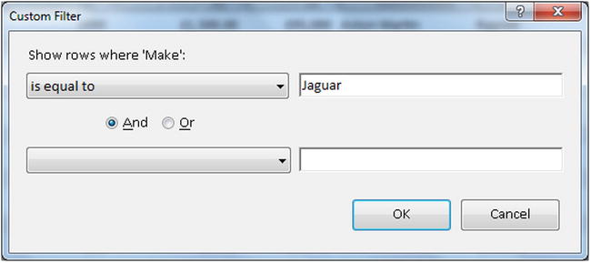
Figure 9-31. The Filter popup
- Click OK.
The data will be filtered to show only records where the make is Jaguar.
The principal advantage of using advanced filters with text columns is that it can simply be faster to set a filter by typing it in. This also allows you to enter up to two filters by selecting the And option in the Custom Filter dialog and setting the second row in the dialog to filter on another element.
Advanced filters become more useful when applied to numeric data. This is principally because they let you define a range of data—you assign a lower and upper threshold to subset the data if you prefer. To see this in action, let’s filter the data for the SalesData table to show only sale prices between £50,000.00 and £100,000.00.
- Click on the popup icon to the right of the column name (using the SalePrice column here).
- In the filter popup, click on the popup triangle for Number Filters.
- Click Greater Than Or Equal To. The Custom Filter dialog appears.
- Leave Greater Than Or Equal To on the left and enter 50000 in the upper text box on the right.
- Make sure that And is selected in the center of the Custom Filter dialog.
- Select Less Than Or Equal To from the lower of the two popups.
- Enter 100000) in the lower text box on the right. The Custom Filter dialog should look like Figure 9-32.
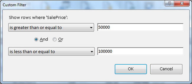
Figure 9-32. The Custom Filter dialog for a range of numbers
- Click OK.
The data will be filtered to show only records where the sale price is between £50,000.00 and £100,000.00.
This is not, of course, the only way in which numbers can be filtered. You can look for
- Numbers above a certain limit (by setting the lower threshold only to Greater Than or Greater Than Or Equal To)
- Numbers below a certain limit (by setting the lower threshold only to Less Than or Less Than Or Equal To)
- Numbers outside a specified range, by inversing the use of greater than and less than in steps 3 and 6 in the preceding exercise
- Numbers not equal to a certain value by using the Not Equal To option.
To modify an existing custom filter, all you have to do is click on the popup icon to the right of the column name, click on the popup triangle for Number Filters, and select Custom Filter. The filter that you last specified will reappear and you can tweak it as you see fit.
Filtering by date is very similar to filtering by numbers. You can select date ranges or all elements where a date is greater or lesser than a certain date. The available options (which include a superb range of instant presets) are outlined in Table 9-14.
Table 9-14. Date Custom Filters
|
Filter Element |
Description |
|---|---|
|
Equals |
Filters data to include only records for the selected date |
|
Before |
Filters data to include only records up to the selected date |
|
After |
Filters data to include only records after the selected date |
|
Between |
Lets you set an upper and a lower date limit to exclude records outside that range |
|
Tomorrow |
Filters data to include only records for the day after the current system date |
|
Today |
Filters data to include only records for the current system date |
|
Yesterday |
Filters data to include only records for the day before the current system date |
|
Next Week |
Filters data to include only records for the next calendar week |
|
This Week |
Filters data to include only records for the current calendar week |
|
Last Week |
Filters data to include only records for the previous calendar week |
|
Next Month |
Filters data to include only records for the next calendar month |
|
This Month |
Filters data to include only records for the current calendar month |
|
Last Month |
Filters data to include only records for the previous calendar month |
|
Next Quarter |
Filters data to include only records for the next quarter |
|
This Quarter |
Filters data to include only records for the current quarter |
|
Last Quarter |
Filters data to include only records for the previous quarter |
|
Next Year |
Filters data to include only records for the next year |
|
This Year |
Filters data to include only records for the current year |
|
Last Year |
Filters data to include only records for the previous year |
|
Year To Date |
Filters data to include only records for the calendar year to date |
|
Custom Filter |
Lets you set up a specific filter for two possible date ranges |
![]() Note All the date presets (those that refer to a week, month, quarter, or year) imply dates relative to the current system date.
Note All the date presets (those that refer to a week, month, quarter, or year) imply dates relative to the current system date.
Conclusion
Now you can import data into PowerPivot from multiple sources and keep it regularly updated so that you are always looking at the most recent information. Not only that, but you can filter and sort your data, as well as format it and fix row titles to help you look more deeply into the data. All in all, you now have a powerful set of tools in your armory that you can use to begin analyzing extensive data sets.
However, getting an initial data set into PowerPivot is only the first part of the process. You now need to be able to link the tables that you have imported in order to query them efficiently. Then you have to be able to extend the data set with any calculations that you need to convert raw data into accurate analysis. You also need to prepare certain columns to enhance the final display in Power View. These techniques are the subjects of the next two chapters.