
CHAPTER 9
Sensors
I CONSIDERED TITLING this chapter “Nuts and Bolts” because it is all about a variety of HA sensors that I believe make up the nuts and bolts of an HA system. I have discussed various sensors in previous chapters but really didn’t provide too much discussion on how they work or are interfaced with a RasPi. This chapter provides the necessary background on how to connect and program several commonly used sensors found in HA systems. Hopefully, it will also provide enough guidance for you to be able to connect different sensors using similar interface connections.
Temperature and Humidity Sensors
I will cover a variety of temperature and humidity sensors to provide you with a good understanding of how these sensors function. Each sensor provides both temperature and humidity readings, but they provide the data to a RasPi using different data protocols. You will gain a good understanding of the different interface protocols by reading all these sensor discussions. You should also consider duplicating one or more of the demonstrations to further improve your knowledge and confidence in using this sensor type.
Parts List

DHT11
A number of fairly inexpensive temperature and humidity sensors are readily available for purchase. They fall into one of three categories based on how they are designed:
![]() Capacitive. These are thin-film capacitance-based sensors with an element bonded to a monolithic circuit that provides a voltage output as a function of relative humidity.
Capacitive. These are thin-film capacitance-based sensors with an element bonded to a monolithic circuit that provides a voltage output as a function of relative humidity.
![]() Resistive. These measure the change in electrical impedance of a hygroscopic medium such as a conductive polymer, salt, or treated substrate.
Resistive. These measure the change in electrical impedance of a hygroscopic medium such as a conductive polymer, salt, or treated substrate.
![]() Thermal conductivity. These consist of two matched negative temperature coefficient (NTC) thermistor elements in a bridge circuit; one is hermetically encapsulated in dry nitrogen, and the other is exposed to the environment.
Thermal conductivity. These consist of two matched negative temperature coefficient (NTC) thermistor elements in a bridge circuit; one is hermetically encapsulated in dry nitrogen, and the other is exposed to the environment.
I will be using the DHT11 resistive sensor because it is commonly used, quite inexpensive, and has good Python libraries readily available. Figure 9-1 shows two DHT11 versions that can be easily purchased. The unit on the left is the board version, and the unit on the right is the standalone component version. I used the component version in this chapter’s demonstration.
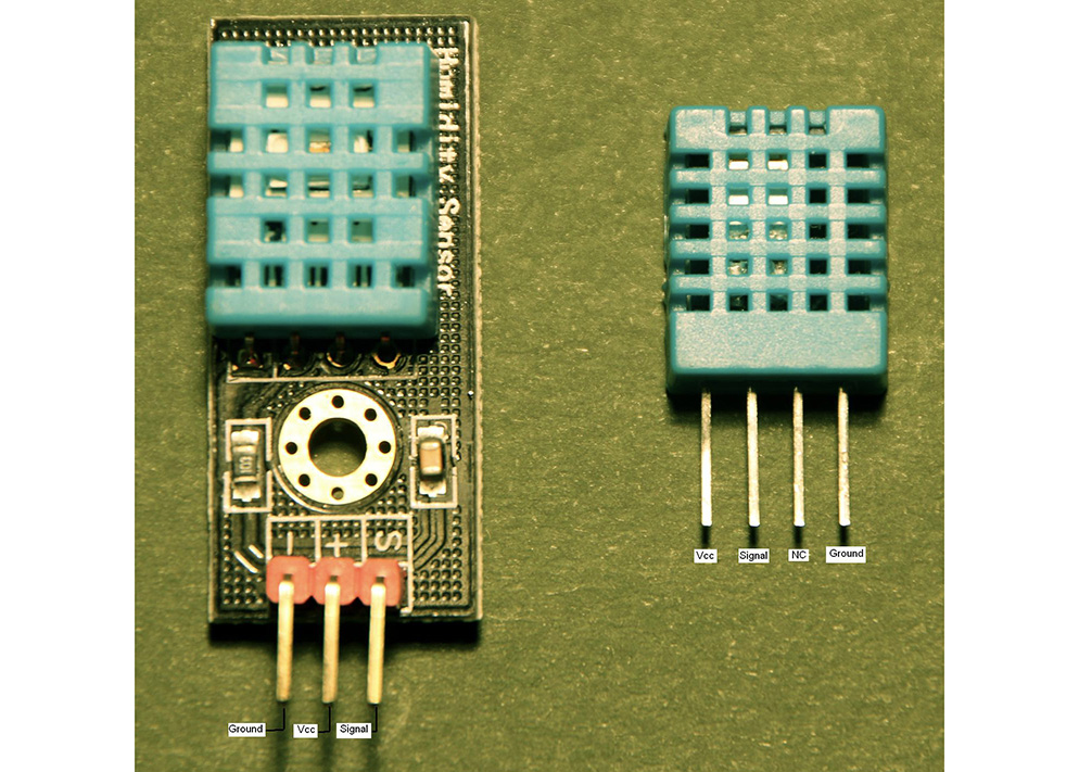
Figure 9-1 DHT11 versions.
The DHT11 specifications are
![]() Very low cost
Very low cost
![]() 3 to 5 V of power
3 to 5 V of power
![]() 3- to 5-V I/O levels
3- to 5-V I/O levels
![]() 2.5 mA of maximum current use during conversion or requesting data
2.5 mA of maximum current use during conversion or requesting data
![]() 20 to 80 percent humidity readings with ±5 percent accuracy
20 to 80 percent humidity readings with ±5 percent accuracy
![]() 0 to 50°C temperature readings with ±2°C accuracy
0 to 50°C temperature readings with ±2°C accuracy
![]() Maximum of 1-Hz sampling rate
Maximum of 1-Hz sampling rate
![]() Size 15.5 × 12 × 5.5 mm (component version)
Size 15.5 × 12 × 5.5 mm (component version)
![]() Four I/O pins with 0.1-inch spacing
Four I/O pins with 0.1-inch spacing
There is only one signal lead on the sensor, which functions as both an input and output for digital signals. This arrangement is often referred to as a one-wire protocol because it only uses one signal lead for both input and output data transmission. Unfortunately, this is often confused with the 1-Wire Protocol, which is another single-wire I/O data transmission protocol. The 1-Wire Protocol is a device communications bus system designed by the Dallas Semiconductor Corp. that provides low-speed data, signaling, and power over a single wire. Both single-wire protocols perform I/O operations, but they use different timing and data-level representations. The software library for the one-wire protocol has been specifically designed to operate with only that protocol.
Physical Setup
Figure 9-2 is a Fritzing diagram showing how to connect a DHT11 with a RasPi. It is very important to connect a 10-kΩ pull-up resistor between the signal lead and the 5-V supply. The one-wire protocol will not work without this resistor installed.
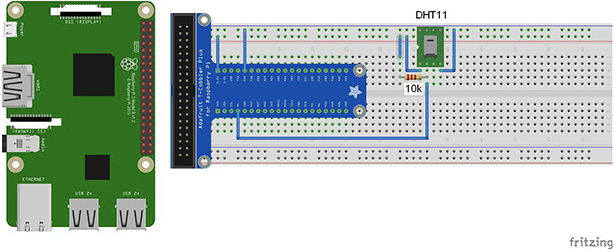
Figure 9-2 Fritzing diagram for connecting a DHT11 with a RasPi.
Note that the supply to the sensor is 5 V, but the signal output level is 3.3 V, making the sensor completely compatible with the RasPi’s GPIO pin voltage levels. The DHT11 signal-out lead connects to RasPi GPIO pin 4.
Software Installation
You should follow this terminal command sequence to install the software required to operate a DHT11 sensor using Python:
1. Installs the git application, which is required for the cloning operation:
sudo apt-get install git-core
2. Clone the Adafruit DHT11 software from the GitHub website:
![]()
3. Change into a new directory created from the clone operation:
cd Adafruit_Python_DHT
4. Build the software:
![]()
5. Run the setup script:
sudo python setup.py install
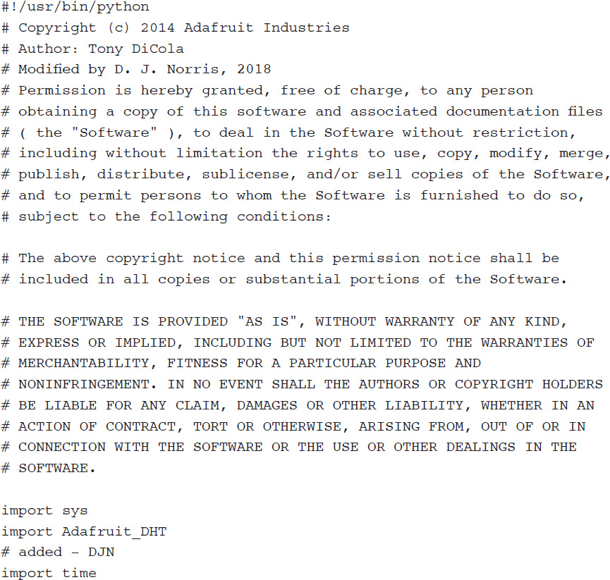
There is a file named AdafruitDHT.py in the Examples directory, which is located in the Adafruit_Python_DHT directory. This file will be used as a script to demonstrate the sensor’s operation. You should first modify this file using the nano editor to incorporate the changes I have noted in the following listing. The modifications cause the script to continuously run as well as display temperatures in ºF. You can leave out that last change if you prefer to display temperatures in ºC.

Test Run
I ran the test script by entering the following terminal commands:
cd Adafruit_Python_DHT/examples
python AdafruitDHT.py 11 4
Figure 9-3 shows the script output after running for several hours.

Figure 9-3 AdafruitDHT.py script screen display.
TMP36
Analog Devices’ TMP36 is my favorite temperature sensor, mainly because it is quite accurate and also extremely inexpensive. It is shown in Figure 9-4.
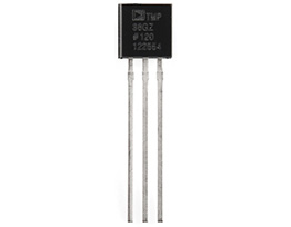
Figure 9-4 Analog Devices TMP36 temperature sensor.
The TMP36 is housed in a standard TO-92 form factor, which is also common to most plastic-encased transistors. The TMP36 is far more complex than a simple transistor in that in contains circuits to both sense ambient temperature and convert that temperature to an analog voltage. The functional block diagram is shown in Figure 9-5. The TMP36 has only three leads, which are shown in the bottom view in Figure 9-6.

Figure 9-5 TMP36 functional block diagram.

Figure 9-6 TMP36 bottom view showing external leads.
Table 9-1 provides details concerning these three leads, including important limitations.
Table 9-1 TMP36 Pin Details

The voltage representing the temperature depends on the TMP36 supply voltage, which must be considered when converting the VOUT voltage to the equivalent real-world temperature. I do account for this in the software that converts the VOUT voltage to an actual temperature. Figure 9-7 is a graph of the signal pin voltage versus temperature using a 3-V supply voltage.

Figure 9-7 Graph of VOUT voltage versus temperature for a +VS = 3 V.
The actual temperature measurement range for the TMP36 is -40 to +125°C, with a typically accuracy of ±2°C and a 0.5°C linearity. These are good specifications considering that the cost of the TMP36 is typically less than $2. The TMP36 range, accuracy, and linearity are well suited for a home temperature monitoring system.
Analog-to-Digital Conversion
The RasPi does not contain any means by which analog signals can be processed. This means that an analog-to-digital converter (ADC) must be used before the RasPi can handle this sensor’s signal.
I used a Microchip MCP3008, which is described on the Microchip datasheet as a 10-bit SAR ADC with SPI data output. Translated, this means that the MCP3008 uses a successive approximation register (SAR) technique to create a 10-bit digital result, which, in turn, is output in a serial data stream using the Serial Peripheral Interface (SPI) protocol. How the SPI protocol functions will be addressed after the sidebar that follows. The inexpensive MCP3008 ADC chip has impressive specifications despite its very low cost. Figure 9-8 shows the package form and pin-out for this chip.

Figure 9-8 MCP3008 package form and pin-out.
The MCP3008 chip used in this chapter’s project is in a dual-in-line package (DIP), which means that I had to use a solderless breadboard to interface it with the RasPi. I encourage you to read the following sidebar if you are interested in how the MCP3008 accomplishes the analog-to-digital conversion. There will be no loss of continuity if you choose to skip the sidebar, however.
Inner Workings of the MCP3008 ADC Microchip
I will refer to the MCP3008 functional block diagram shown in Figure 9-9 throughout this discussion. The analog signal is first selected from one of eight channels that may be connected to the input channel multiplexer. Using one channel at a time is called operating in a single-ended mode. The MCP3008 channels can be paired to operate in a differential mode if desired. A single configuration bit named SGL/DIFF selects single-ended or differential operating mode. Single-ended is the mode used in this project.
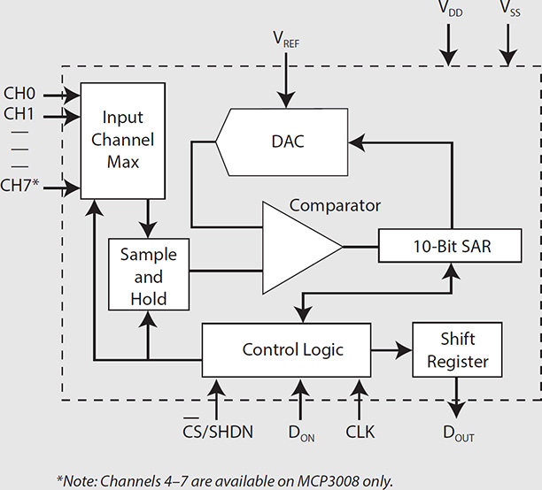
Figure 9-9 MCP3008 functional block diagram.
The selected channel is then routed to a sample-and-hold circuit, which is one input to a comparator. The other input to the comparator is from a digital-to-analog converter (DAC), which receives its input from a 10-bit SAR.
Basically, the SAR starts at a 0 count output and rapidly increments to a maximum of 1,023, which is the largest number that can be represented with 10 bits. Each count increment also increases the voltage appearing at the other comparator’s input. The comparator will trigger when the DAC voltage precisely equals the sampled voltage, and this will stop the SAR from any further incrementing. The digital number that exists on the SAR at the moment the comparator triggers is the ADC value. This number is then output, 1 bit at a time, through the SPI circuit, which I discussed below. All this takes place between sample intervals. The actual voltage represented by the ADC value is a function of the reference voltage Vref connected to the MCP3008. In our case, Vref is 3.3 V; therefore, each bit represents 3.3/1,024, or approximately 3.223 mV. For example, an ADC value of 500 would represent an actual voltage of 1.612 V, which was computed by multiplying 0.003223 by 500.
Serial Peripheral Interface
The SPI is one of several data communication channels that the RasPi supports. It is a synchronous serial data link that uses one master device and one or more slave devices. A minimum of four data lines are used with SPI, and Table 9-2 shows the names associated with the master (RasPi) and the slave (MCP3008) devices.
Table 9-2 SPI Data Line Descriptions

Figure 9-10 is a simplified block diagram showing the principal components used in an SPI data link. There are usually two shift registers involved in the data link, as shown in the figure. These registers may be hardware or software depending on the devices involved. The RasPi implements its shift register in software, whereas the MCP3008 has a hardware shift register. In either case, the two shift registers form what is known as an interchip circular buffer arrangement that is the heart of the SPI.

Figure 9-10 SPI simplified block diagram.
Data communication is initiated by the master by first selecting the required slave. The RasPi selects the MCP3008 by bringing the SS line to a low state or 0 VDC. During each clock cycle, the master sends a bit to the slave, which reads it from the MOSI line. Concurrently, the slave sends a bit to the master, which reads it from the MISO line. This operation is known as full duplex communication, that is, simultaneous reading and writing between master and slave.
The clock frequency used depends primarily on the slave’s response speed. The MCP3008 can easily handle bit rates of up to 3.6 MHz if powered at 5 V. Because we are using 3.3 V, the maximum rate is a bit less at approximately 2 MHz. This is still very quick and will process the RasPi input without losing any data.
The first clock pulse received by the MCP3008 with its chip select (CS) held low and Din high constitutes the start bit. The SGL/DIFF bit follows next and then 3 bits that represent the selected channel(s). After these 5 bits have been received, the MCP3008 will sample the analog voltage during the next clock cycle.
The MCP3008 then outputs what is known as a low null bit, which is disregarded by the RasPi. The following 10 bits, each sent on a clock cycle, are the ADC value with the most significant bit (MSB) sent first down to the least significant bit (LSB) sent last. The RasPi will then put the MCP3008 CS pin high, ending the ADC process.
Initial Test
Initial testing involves both creating a hardware circuit and establishing the proper Python software environment.
Hardware Setup. I will first discuss the hardware circuit because it is relatively straightforward. Figure 9-11 shows the test schematic for the T-Cobbler, MCP3008, and TMP36. I connected the TMP36 Vout lead to the MCP3008 Channel 0 input, which is pin 1, as shown in Figure 9-8.

Figure 9-11 Test schematic.
The actual physical setup is shown in Figure 9-12. On the right side of the breadboard, you can see the TMP36 sensor connected with three jumper wires to the other breadboard circuitry.

Figure 9-12 Physical test setup.
Table 9-3 shows the equivalents between the ADC count, sensed temperature, and voltage. Use these values to verify that the TMP36 sensor is accurately measuring the ambient temperature. You can easily add a calibration factor if the measured temperature does not equal the true temperature as measured by a separate calibrated thermometer.
Table 9-3 ADC Count, Voltage, and Temperature Equivalents

Software Setup. You next need to load the Python developer libraries, which will allow you to support the script to run the SPI circuit. Install the Python development libraries by entering
sudo apt-get install python-dev
The following test script displays a continuous stream of temperature values generated by the TMP36 sensor. The program is named TMPSensor.py and is available for download from this book’s website, www.mhprofessional.com/NorrisHomeAutomation. The code follows the MCP3008 ADC configuration guidelines and SPI protocol, as discussed earlier. The code employs a “bit-banging” approach to SPI interface implementation. This approach makes running the script independent of any prerequisite SPI driver installations, which I felt made the test process as simple as possible.

Run the script by entering
sudo python TMPSensor.py
Figure 9-13 is screen shot of a portion of the program output with the TMP36 sensor measuring ambient room temperature. In the figure, the number in the left-hand column is the raw count coming from the MCP3008 ADC. The number in the middle column is the equivalent voltage for the raw count. The right-hand column shows the equivalent temperature for the voltage in degrees Celsius.
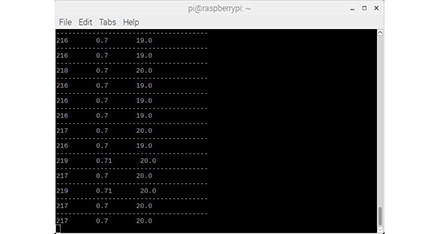
Figure 9-13 Initial test results.
Passive Infrared Sensor
This sensor is designed to sense the presence of humans or other warm-blooded mammals. Figure 9-14 shows a typical passive infrared (PIR) sensor, which is inexpensive and commonly used for both motion and occupancy detection.
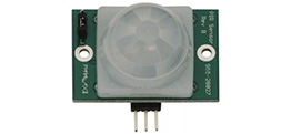
Figure 9-14 Passive infrared sensor.
This sensor’s ratings, pin connections, and range jumper settings are detailed in Figure 9-15, which comes from the manufacturer’s datasheet.
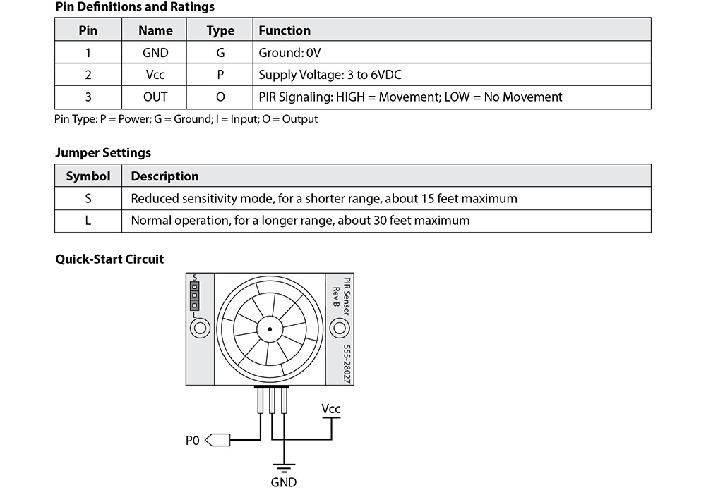
Figure 9-15 Sensor ratings, pin connections, and jumper settings.
The PIR sensor uses a crystalline material that generates an electric charge when exposed to infrared energy. The amount of energy generated is proportional to the size and thermal properties of nearby objects. Environmental conditions also affect the sensor, including ambient light and heat sources. A Fresnel lens located in front of the active element that focuses all incoming infrared signals. An onboard electronic amplifier is triggered when rapid infrared signal changes are detected. The detection range for this particular sensor may be modified by repositioning a jumper located in the upper left-hand corner, as shown in the quick-start circuit of Figure 9-15. One position is the so-called normal position and provides a nominal 30-foot detection range. The other position is the reduced-sensitivity one, where the detection range is half the normal range, or 15 feet. That position would be appropriate for indoor use in a normal-sized room.
This type of sensor is affected by ambient temperature, which should not be surprising considering that it basically works by detecting rapid temperature changes. Figure 9-16 is a graph that shows the effects of ambient temperature on the sensor for both the normal and reduced-sensitivity jumper settings.

Figure 9-16 Ambient temperature versus detection range.
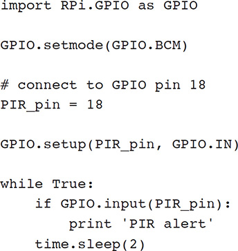
Test Script
There are no special software dependencies that need to be installed in order to support this sensor. It functions just fine with the normal RPi.GPIO library that I have used in previous chapters, which is the only library needed to interface with the RasPi GPIO pins. The following is the Python script I wrote to test this sensor. I named this script PIRTest.py, and it is available from this book’s companion website, www.mhprofessional.com/NorrisHomeAutomation.
Test Run
The sensor has some dim red LEDs in the Fresnel lens that will light for approximately 40 seconds when power is first applied to the sensor. This is the self-calibration period that the sensor requires for normal operations. It will be ready to run the script after this period ends and the LEDs go out. You can run the script by entering this command:
python PIRTest.py
Now wave your hand in front of the sensor, and you should see the message PIR alert appear in the terminal window. It may reappear because the sensor requires several seconds to reset after the initial motion ceases. The LEDs in the Fresnel lens will also light when motion is detected.
This test demonstrates that this type of sensor is quite simple in its operation and has little flexibility other than a range sensitivity setting. Nonetheless, this sensor type has been applied to a vast variety of home lighting applications, including driveway and porch lighting. However, the question naturally arises, what type of sensor is available if you need a more precise measure of a person’s distance from the sensor? The next section addresses this issue.
Ultrasonic Sensor
An ultrasonic sensor provides for actual distance measurements between a target and the sensor. Figure 9-17 shows front and back views of the ultrasonic sensor used in this demonstration.
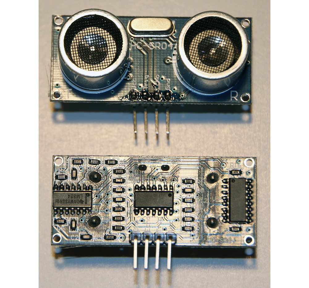
Figure 9-17 Ultrasonic sensor front and back views.
The ultrasonic sensor contains an embedded microprocessor as part of the encapsulated sensor hardware. This processor controls the ultrasonic transmitter and receiver transducers that physically measure distance by bouncing discrete ultrasonic sound wave pulses off objects and timing how long the sound pulse takes to make the round-trip transit. The distance is easily calculated because the speed of sound in air is relatively constant. This is very similar to how bats navigate in caves and attics. Figure 9-18 is a block diagram of the sensor showing how it functions.
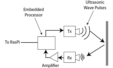
Figure 9-18 Ultrasonic sensor block diagram.
The embedded processor generates an ultrasonic pulse when triggered by the RasPi. It also generates an output pulse if a return echo is detected. A RasPi GPIO pin is used to trigger a 40-kHz ultrasonic burst. The sensor then “listens” for an echo return and sets another RasPi GPIO pin high. Software running on the RasPi detects the time differential between the trigger pulse and the echo return pulse and converts that time interval into an equivalent distance between the sensor and the reflecting target. The operational block diagram in Figure 9-19 illustrates this process and identifies the sensor and RasPi pins used for the interconnections. However, an important level-shifter chip is not shown in this figure but is shown in the schematic in the next section.

Figure 9-19 Operational block diagram.
The ultrasonic sensor measures distances from 3 to 250 centimeters (cm) with an accuracy of approximately ±2 cm, which is less than a 1-inch error. Distance measurements also depend on the size and texture of the object that reflects the sound pulses. A wall provides excellent reflections, whereas a stuffed toy would be more problematic.
Physical Setup
This sensor requires 5 V for power and returns 5-V pulses for the echo signal. This voltage level is incompatible with a RasPi GPIO level input and must be reduced to 3.3 V or else damage will occur to the RasPi. I elected to use a level-shifter module to accomplish this reduction. Figure 9-20 is the interconnection schematic.

Figure 9-20 Interconnection schematic.
NOTE: You can also use a simple resistive divider to lower the input voltage to pin 24, but I already had a level-shifter module available and felt that it was a better solution to this problem. However, Figure 9-21 is a schematic for the resistive voltage divider for those of you who may choose to use that alternative.

Figure 9-21 Resistor voltage divider.
Figure 9-22 shows the breadboard ready for a test. You should place the sensor near the outer edge of the breadboard, clear of any other components or wires. I placed a small box in front of the sensor as well as a ruler calibrated in centimeters between the sensor and the box target.

Figure 9-22 Physical setup.
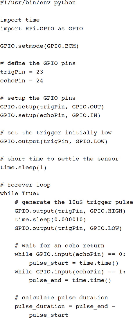
Test Script
No special software dependencies are needed to support this sensor. It functions with the normal RPi.GPIO library, which that I have used in previous demonstrations. The following is the Python script I wrote to test this sensor. I named this script UltrasonicTest.py, and it is available on this book’s website.

Test Run
You can run the script by entering this command:
python ultrasonicTest.py
Figure 9-23 shows the script output using a good reflective target set at about 10 cm from the sensor. The displayed values very accurately correspond with the actual distance between the sensor and target. I then tried measuring the distance between the room ceiling and the sensor. I again found a very accurate measurement result.

Figure 9-23 Script output.
The most popular form of object detection in HA applications has been with PIR sensors, which I discussed earlier. While reliable, they are easily activated and fooled by temperature or light changes, flying insects, and small animals. In contrast, ultrasonic detection is more reliable because it senses motion or presence of an object by the reflection of transmitted ultrasonic bursts. Ultrasonic presence detection can be a very useful tool in building automation and boosting energy savings through the control of lights, heating, and other energy consumers. Another potential HA application is parking detection, where a driver can be guided to very accurately park a car in a garage. Ultrasonic detectors also can be used in safety applications in which very reliable object detection is a high priority. A good application might be swimming pool surveillance, where it is critical to generate an alert or alarm if a small child attempts to enter an unattended pool.
Summary
This chapter discussed popular sensors often used in HA systems. My primary purpose was to explore how different sensors operate and how they can be interfaced with a RasPi.
The first sensor demonstrated was the DHT11, which is an integrated humidity and temperature sensor. It works using a software library provided by Adafruit, which has a single-line command to input a set of humidity and temperature readings from the sensor.
The next sensor described was a very inexpensive temperature sensor named TMP36. It outputs an analog DC voltage proportional to temperature. This situation requires the use of an analog-to-digital converter (ADC) between the sensor and the RasPi. I described how to set up a MCP3008 ADC to do the analog-to-digital conversion. I explained how the ADC used the SPI protocol to communicate with the RasPi. The project demonstration successfully measured ambient temperature using the TMP36, MCP3008, and RasPi.
I next demonstrated a passive infrared (PIR) sensor. This sensor uses a crystalline sensing element to detect changes in ambient heat signatures. It is very useful for motion-detection applications.
The last sensor demonstrated used ultrasonic acoustic pulses to measure distances between the sensor and a target. This technique is akin to how bats echo-locate around their environment. This sensor is very accurate and reliable and is independent of ambient temperature, which adversely affects PIR sensors.