3. Projecting Base Compensation Costs

Total compensation costs are often the highest direct and indirect expense in any organization. However, an analysis of the various elements of the total compensation is not always accomplished in whole or in part with analytical thoroughness. But because it can be the highest line item expense, understanding and projecting the true costs is of strategic and operational importance. This chapter presents a framework for analyzing each component of the total base compensation equation. It also provides analytical techniques to plan and forecast these expenses.¹ The chapter also covers base salary projections. Other chapters, where appropriate, deal with projecting the other elements of the total compensation system.

¹ Adapted from an article written by Biswas, B.D., and Hestwood, T. in the Compensation Review Journal in 1979. Copyright currently held by Sage Publications. Author use accepted by Sage Publications.

You need to understand the various expense elements to accurately forecast compensation expenses. This understanding is important because these expenses are critical for long-term financial planning. Projecting these expenses is of strategic importance because accuracy here assists with the setting of the right “selling price” for a product or service, which then leads to determining the optimum financing and investing strategies. Furthermore, accuracy here leads to effective talent management strategies. Forecasting these expenses with accuracy also enables better annual financial budgeting and cash budgeting. The appendix, at the end of this chapter, provides a specific example of the direct relationship of salary planning to the determination of the annual cash requirements of a business.

Now, it is important to understand the connections between accurate compensation cost planning and financial planning. Exhibit 3-1 demonstrates these connections.

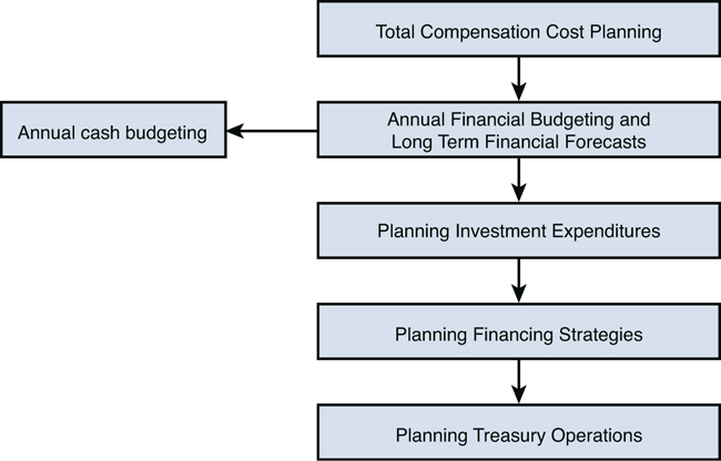
Exhibit 3-1. The Important Connection between Compensation Expense Planning and Financial Planning

Note here that if total compensation expenditures are indeed the most significant element of total expenditures, then being accurate with those projections will enhance the credibility and accuracy of the total financial planning system.

Before we start the planning exercise, it is again important to take a look at the various compensation and benefits cost elements. We do so in Exhibit 3-2.

Exhibit 3-2. Elements of the Total Compensation Framework (continuing the discussion from Chapter 1)

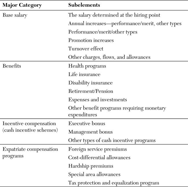
In the discussions about the projections of total compensation forecasting, expenditures normally paid via expense reimbursements or those directly paid by third-party administrators (TPAs) are excluded. These expenditures are as follows:

• Executive perquisites (the imputed value of which would be included as taxable income)

• Pension payments

• Medical insurance reimbursements

• Other insurance payments paid by TPAs and insurance companies

• Expatriate tax payments

• Company reimbursement to service providers on behalf of employees

The focus here is on all payments processed by the payroll department. Employee payments processed by payroll departments are subject to federal and state tax withholding requirements, whereas payments made by expense reimbursement are not subject to withholding taxes.

Organizations execute these actions in a variety of ways. One way to allocate increases is a salary or merit increase matrix. These are guidelines that assist in the determination of individual increases based on performance and the employee’s salary range position. Using these guidelines, organizations forecast the cost of the salary increase program. Yet another method used to distribute increases to employees is based on performance ratings and resulting in a specific yearly average amount and also the time between increases. This average can vary for different groups of employees. The cost is calculated by multiplying the annual increase percentage by the base salary for each employee group at the beginning of the year.

Nevertheless, existing costing procedures are normally deficient in one or more of the following areas:

• They do not account for employee turnover.

• They ignore or inaccurately predict the net changes in employee population.

• They overlook deviations from approved practices.

Employee turnover can have a significant impact on anticipated salary expenditures because of the differences in the salaries of employees leaving and those employees joining the organization. Turnover lowers costs because employees who terminate usually are compensated at higher levels than those who replace them. In fact, because of turnover in some companies, salary programs add zero dollars to total payroll.

However, the impact of turnover is generally more involved than that, because there is rarely the simple replacement of one employee by another employee. Employees are not always directly replaced by other employees for the same job. There is a constant change in the mix of various kinds of employees and jobs. The effect of turnover can best be determined by an analysis of the relationship of new hire and terminee salaries.

The cost effects of population changes can prove particularly difficult to forecast because they often vary substantially from year to year depending on business, financial, and economic conditions. This information can be gathered from an organization-wide human resource (HR) planning and forecasting system (as discussed in Chapter 2, “Business, Financial, and Human Resource Planning”). But where forecasting data is not available, or where the forecasting process is not synchronized with compensation planning, the information must be derived from historical trend data for employee demographic changes.

Irrespective of the spending controls established, deviations from expected levels of spending often occur. It occurs quite often when managers are slow to adjust their spending to reflect the program changes and new programs. Some companies actually encourage deviations from policy in special employment cases. There is a belief that supervisors should not be subjected to strict spending controls. If measurable deviations occur consistently, provisions should be made for anticipating the cost impact by reviewing the historical relationships between authorized and actual merit increases.

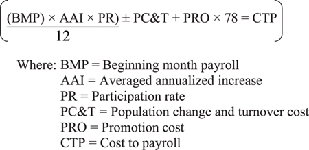
Exhibit 3-3. Payroll Forecasting Formula

Beginning month payroll (BMP) is the total base monthly payroll at the beginning of the program year. Most organizations have this information available in various HR and financial (payroll) electronic systems.

To demonstrate the forecasting methodology, let’s consider an example. This example assumes that there are 100 employees with a payroll of $500,000 a month.

The average annualized increase (AAI) combines the effect on payroll of the expected average time interval between increases and the average amount of the increase during a given year or fiscal year. The annualized increase calculation determines the full-year impact of increases granted throughout the year. It also takes into account the higher base salary of employees who receive more than one increase within a year. This is because the interval between increases is less than 12 months for employees who receive more than one increase during a 12-month period. In the example, we assume that the expected average increase is 7%, with an interval between increases of 9 months. In most companies these increases would be based on performance (commonly termed merit increases). Exhibit 3-4 explains how the annualized increase is obtained.

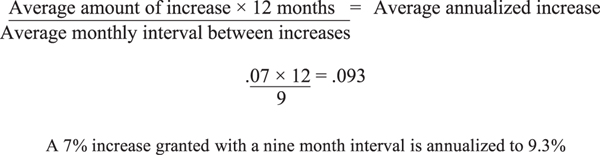
Exhibit 3-4. Determining the Annualized Increased Component

When increases are granted at intervals that are not approved, the average will need to be adjusted. These deviations arise mainly in organizations that are decentralized with local autonomy. If there is historical evidence of a consistent deviation pattern in the increase interval, then an adjustment should be built into the calculations proactively.

In this case, the example assumes that an analysis of the data indicates a need for an adjustment in the expected interval between increases. You can obtain this information by analyzing the data on the historical relationship between the actual and approved interval between increases.

You might find, for example, that last year the actual average interval was 11.5 months but the approved interval was 12 months. This year, the approved program’s average interval is 9 months. If the past relationship between the approved and actual interval is a valid guide for the future, you can set up a simple ratio equation and solve for the expected actual interval for the forecasting exercise.

Exhibit 3-5 presents this calculation. In the example, the expected interval is 8.63 months. This corrected interval can be inserted in place of 9 months in the annualizing formula to yield an AAI of 9.7% rather than 9.3%.

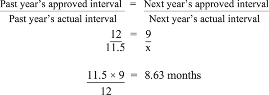
Exhibit 3-5. Adjustment for Approved Versus Actual Interval

Participation rate (PR) is defined as the ratio of actual salary actions (increases) granted to employees compared to all employees eligible to receive increases. Participation is significant because if not all the possible salary increases are awarded, a smaller portion of base payroll than expected is actually increased. If this situation occurs, an adjustment must be made that reduces the projected expenditure. Unless an organization sets a specific participation rate objective, this information has to be obtained from a historical comparison of what actually occurred at year end to the number of possible actions for the year. Consequently, if it is anticipated that only 90% of the employees are going to receive a salary action, the annual merit increase cost must be multiplied by .90 to eliminate the 10% not participating.

After the participation rate is considered, the resulting cost is divided by 12 to obtain a monthly cost. So far in the example, the calculation would read as follows:

($500,000 × .097 × .90) ÷ 12 = $4,041.67 per month – Monthly payroll increase.

The effects of population change and turnover (PC&T) on salary expenses are considered together. In the example we are looking only at an increase in population. However, with minor changes, the procedure can be made to account for declines in population, as well. For this analysis, it is assumed that population change information is derived from historical trends maintained in the human resource information system. The effects of turnover on costs also would be obtained from historical data.

To determine the effects of population change and turnover require that an organization record monthly the salaries of new hires and terminees. Preferably, this data should be collected for at least five years. Exhibit 3-6 illustrates the type of information that should be collected each month.

Exhibit 3-6. Data for PC&T

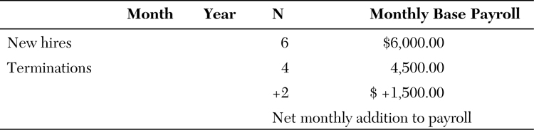
To determine the average monthly additional cost to payroll, all monthly changes to payroll are averaged. Therefore, if the monthly net addition to payroll is $1,500, as shown in the calculation, that amount is added to the formula as the PC&T expense.

If population changes are not expected to follow historical patterns, there must be a way to separate turnover and growth. In the example shown in Exhibit 3-6, it is assumed that all new hires come in at the new-hire average salary of $1,000 per month and that there were two more new hires than terminees (these hires are presumed to be for positions that are newly created). Therefore, in this case, population growth accounts for a change in payroll of $2,000 ($1,000 × 2). But, turnover normally acts to reduce payroll. Because new-hire salaries are lower than those of terminees, there was a cost savings of $125 per replacement hire (average new hire cost of $1,000 versus average terminee cost of $1,125, a savings of $125 per replacement hire). This savings multiplied by the number of persons directly replaced (we assume four of the six new hires were replacing four who terminated) gives total monthly turnover savings of $500. Thus, the two growth hires were brought in at a cost of $2,000 ($1,000 × two brand new employees) and the four who were replaced came in at a lower salary ($1,000 per month), but they replaced four employees whose salaries averaged $1,125 per month, which gives a savings of $125 per replacement hire for a total of $500 for four employees. The $2,000 per month additional hire cost is reduced by $500 per month to result in a payroll increase of $1,500 per month.

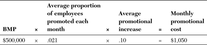
Promotion (PRO) expenses are determined by examining historical data to find the number of employees getting a promotion each month and the average promotional increase. Exhibit 3-7 shows if 2.1% of the population is promoted each month and the average increase of those being promoted is 10%, the monthly promotional cost is $1,050.

Exhibit 3-7. Calculating Promotion Costs

The factor of 78 shown in the costing formula is used to convert the monthly expense to an annual expense; 78 is the total number of times the monthly expense has to be incurred if the expense is being determined for a year. For instance, the salary-increase dollars paid in January will be paid 12 times, the salary-increase dollars paid in February, 11 times, and so forth. This phenomenon is described in more detail in the appendix to this chapter.

The various components of the costing formula can now be shown together. If you insert the figures discussed previously into the formula shown in Exhibit 3-3, it reads as follows:

[($500, 000 × .097 × .90) ÷ 12 + $1,500 + $1,050] × 78 = $482,625

Therefore, an additional $482,625.00 (CTP) will be spent on base salaries in the coming year. From an annual payroll of $6,000,000 at the start of the year, the expense rises to $6,482,625 at year end, an increase of 8.0% ($482,625 ÷ $6,000,000) on an annual basis and 14.85% ($6,188 × 12 ÷ $500,000) on a monthly basis. The $6,188 is calculated in this manner: [($500,000 × .097 × .90) ÷ 12] + $1,500 + $1,050 = $6,188

Another example demonstrates the calculations discussed so far. The costing technique described to project compensation expenses was introduced in the 1970s when the Nixon wage-price controls were in effect. At that time, the concepts of level rise and cost to payroll were introduced. In this cost analysis, the emphasis is on looking at cost increases from both a monthly and annualized basis. The ending monthly figure (as defined by the payroll level rise) indicates the beginning of the next year run rate. The annualized cost increase (as defined by the cost to payroll) indicates the increased annual base compensation expenditures for the current year.

Let’s first take a look at these concepts graphically and then discuss them more fully.

Assume that Paresh Enterprises, Inc. (PEI) has a monthly base payroll of $5,000,000 on 12/31/12. And let’s assume that PEI has an anniversary salary-increase program; that is, employees are granted increases on the anniversary of the hire date. In addition, PEI plans a 5% of base average salary increase program for 2013. So, graphically the base compensation costs of PEI are as shown in Exhibit 3-8.

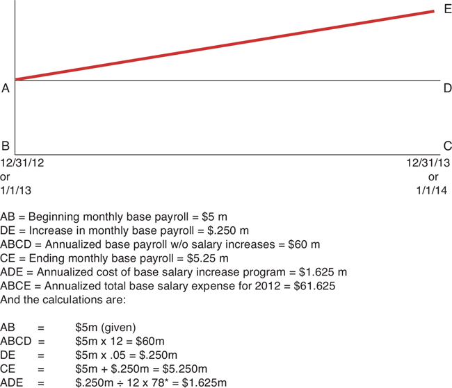
Exhibit 3-8. Base Compensation Costs for PEI

* Look for explanation of this factor in the appendix.

Here is the calculation in percentage terms:

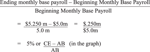
This figure is called level rise or the increase in the monthly base payroll level. This is a number that normally comes from an input provided to the compensation specialist by the budgeting people in the accounting department.

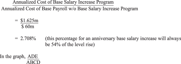
We call this statistic the cost to payroll of the annualized salary increase program. Such a technique for base compensation cost planning enhances the accuracy of the projections of the fixed costs to be incurred by an organization. Such costing accuracy facilitates accuracy cost estimations.

Organizations, both big and small, have to manage their operations by developing accurate financial budgets annually. A major expense that has to be planned by each manager is their employee expenses. And as you have seen, employee expenses can be the largest single line item expense for any organization. Note, as well, that base salary expenses form the major expense within the total compensation framework. Normally, the accounting and finance department provides to department managers budget guidelines for base salary increases that are not coordinated with the HR departments. There are many reasons for this lack of a connection. Common reasons include (1) the HR personnel’s avoidance of anything to do with numbers and (2) the accounting department’s reluctance to communicate with HR departments with respect to accounting and finance matters. However, one of the most important expense categories is people expenses, and therefore there needs to be accounting and finance cooperation on this activity. A financial planning model has been presented in this chapter, which, if put into practice, will greatly enhance fixed compensation estimation accuracy, understanding, and reporting.

• Payroll costing formula

• Average annualized increase

• Approved versus actual increase

• Participation rate

• Promotion costs

• Beginning monthly base payroll

• Payroll level rise

• Cost to payroll

• The 78 factor

• The cash flow impact

• Population change and turnover impact

• Ending monthly payroll

In a survey on compensation planning for 2008, Buck Consultants examined salary management practices among the 415 surveyed organizations (in particular, the timing of annual salary reviews). The Buck survey found that most organizations—over 80% (82.2%)—administer annual salary increases on a focal (or common) review date.² This means that in most organizations employees receive their annual salary increase on a common date, such as January 1, rather than on the annual anniversary of their hire date or when they were promoted into their current positions.

² Koss, Sharon “Which is Best? Anniversary vs. Focal (Common Date)” Performance Reviews, SPHR, CCP (2009): www.kosshrexpert.com/Article-WhichisBest.pdf.

Exhibit 3-9. Employee Salary Increase Dates

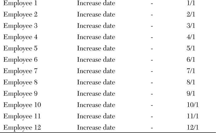
* This example is simplified to demonstrate the concepts.

Now suppose that the annual increase for each employee is 10%. The true cash flow impact of this 10% increase program is demonstrated in Exhibit 3-10.

Exhibit 3-10. The Cash Flow Impact³

³ Thus, the 78 used in Exhibit 3-3.

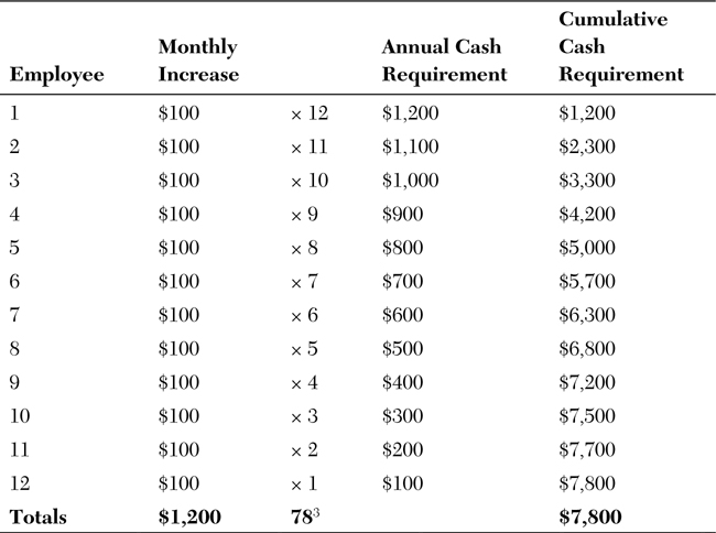
Therefore, an anniversary salary increase generates a cash flow requirement of $7,800 in this hypothetical example, whereas if all employees were granted their annual increases on January 1 the cash flow requirement would be $1,200 × 12 = $14,400. If all employees were granted increases on a focal date of July 1, the cash flow requirement would be $1,200 × 5 = $7,200. And if all employees were granted increases on September 1, the cash flow requirement would be $1,200 × 4 = $4,800.

Note that this is cash flow analysis and not accrued expense analysis. Also note that this type of accounting analysis conducted by a compensation department will add real value to the accounting department’s efforts to do required cash budgeting and planning. Cash management is a critical accounting activity that keeps many a chief financial officer under continuous stress and anxiety. The HR and compensation professionals will certainly “come to the table” when they support the business with this critical cash budgeting and planning activity. The activity becomes all the more important when one considers that in any organization of any size, the distribution of annual salary increases to employees can be one of the highest cash outflow activities.