Chapter 16

BENFORD’S LAW

Major paradoxes provide food for logical thought for
decades and sometimes centuries.

Nicholas Bourbaki

First Digits

At the end of the previous chapter, with the use of the potent Weyl Equidistribution Theorem, we saw that the first digit of powers of 2 are not distributed uniformly over {1, 2, 3, . . . , 9} but rather according to the law

Moreover, we argued that the phenomenon exists equally with 2 replaced by any number that is not a rational power of 10. Perhaps this behaviour is then a property of powers of integers, but then consider the consumption (measured in kilowatt hours) of the 1243 users of electricity of Honiara in the British Solomon Islands in October 1969. Table 16.1 shows the proportion of use beginning with a first digit 1, etc., together with those numbers generated by the logarithmic formula.

Table 16.1.

Of course, the fit is not exact but it is markedly closer than the uniform 0.1111 . . .: something seems to connect mathematical and electrical power. Something does: Benford’s Law.

In 1881 the American mathematician and astronomer Simon Newcomb wrote to the American Journal of Mathematics (Note on the frequency of use of the different digits in natural numbers, 1881, 4(1):39–40) an article which began:

That the ten digits do not occur with equal frequency must be evident to any one making much use of logarithmic tables, and noticing how much faster the first pages wear out than the last ones. The first significant figure is oftener 1 than any other digit, and the frequency diminishes up to 9.

This era, long before the invention of the electronic chip, depended on tables of logarithms for anything other than the simplest calculations; compiled into books these would have been a common sight in any mathematician’s or scientist’s place of work. Newcomb had noticed that the books of logarithms that he shared with other scientists showed greater signs of use at their beginning than they did at their end, but since logarithm tables were arranged in ascending numeric order, this suggested that more numbers with small rather than large first digits were being used for calculation. In the article he suggested an empirical law that the fraction of numbers that start with the digit d is not that intuitively reasonable but that remarkable log₁₀(1+ 1/d).

There was no rigorous justification provided and the idea languished in the mathematical shadows until 1938. It was then that Frank Benford, a physicist at G.E.C., published the paper ‘The law of anomalous numbers’ (Proceedings of the American Philosophical Society, 1938, 78:551–72). In it he had compiled a table of frequency of occurrence of first digits of 20 229 naturally occurring numbers, which is reproduced in table 16.2, and which he had extracted from a wide variety of sources ranging from articles in a selection of newspapers to the size of town populations; the logarithmic not the uniform law held the more convincingly. In particular the penultimate row, which averages the data, is a most excellent fit to the logarithmic model. The phenomenon has subsequently become known as Benford’s Law.

Some Rationale

Two significant and reasonable observations have been made.

One, that if Benford’s Law does hold, it must do so as an intrinsic property of the number systems we use. It must, for example, apply to the base 5 system of counting of the Arawaks of North America, the base 20 system of the Tamanas of the Orinoco and to the Babylonians with their base 60, as well as to the exotic Basque system, which uses base 10 up to 19, base 20 from 20 to 99 and then reverts to base 10. The law must surely be base independent.

The second is that changing the units of measurement must not change the frequency of first significant digits. Ralph A. Raimi, in his survey of progress on the matter (The first digit problem, American Mathematical Monthly, 1976, 83:521–38) wrote the following:

Roger S. Pinkham attributing the basic idea to R. Hamming, put forward an invariance principle attached to another sort of probability model, sufficient to imply Benford’s Law. If (say) a table of physical constants or of the surface areas of a set of nations or lakes, is rewritten in another system of units of measurement, ergs for foot-pounds or acres for hectares, the result will be a rescaled table whose every entry is the same multiple of the corresponding entry in the original table. If the first digits of all the tables in the universe obey some fixed distribution law, Stigler’s or Benford’s or some other, that law must surely be independent of the system of units chosen, since God is not known to favour either the metric system or the English system. In other words, a universal first digit law, if it exists, must be scale-invariant.

Table 16.2.

Recalling our earlier example of electricity consumption, it should not matter whether kilowatt hours were used as a unit or any other alternative. Roger Pinkham, then a mathematician at Rutgers University in New Brunswick (New Jersey), had written a paper demonstrating that scale invariance implies Benford’s Law (On the distribution of first significant digits, Annals of Mathematical Statistics, 1961, 32:1223–30).

In 1995, Theodore Hill of the Georgia Institute of Technology approached matters differently. He showed that, if distributions are selected at random and random samples are taken from each of these distributions, the significant-digit frequencies of the combined sample would converge to conform to Benford’s Law, even though the individual distributions selected may not; a result consistent with that penultimate row of Benford’s table (A statistical derivation of the significant-digit law, Statistical Science, 1995, 10:354–63). In a sense, Benford’s Law is the distribution of distributions.

All of this said, many sets of numbers certainly do not obey Benford’s Law: random numbers at one extreme and numbers that are governed by some other statistical distribution on the other, perhaps uniform or normal. It seems that, for data to conform to the law, they need just the right amount of structure.

An Argument

‘Proving’ Benford’s Law is not like proving a standard mathematical theorem: even stating it properly is difficult, but we will approach it by following the scale-invariance property that it must, in all reason, adhere to.

Table 16.3.

Interval	First significant digit after × 2
[1, 1.5)	2
[1.5, 2)	3
[2, 2.5)	4
[2.5, 3)	5
[3, 3.5)	6
[3.5, 4)	7
[4, 4.5)	8
[4.5, 5)	9
[5, 10)	1

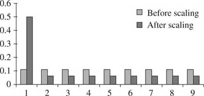
Figure 16.1.

A change of units is achieved by multiplying by some scaling number. Let us assume that the first significant digits of some measurable quantity are originally uniformly distributed and then let us suppose that we change the units by (say) multiplying everything by 2. If the first significant digit of the number in the original units is one of 5, 6, 7, 8, 9, the scaled number must begin with 1, otherwise, the behaviour is shown in table 16.3, which is displayed in the bar chart in figure 16.1. Even if the frequency of first significant digits was uniform before the scaling, it will not be afterwards and we are bound to conclude that equally likely digits are not scale invariant.

We can put forward a general argument using the standard theory of statistical distributions.

Recall that a continuous, nonnegative function φ(x) is the probability density function of a continuous random variable X if P(a X b) = φ(x) dx. Of course, we require that the total area under φ(x) must be 1.

The cumulative density function Φ(x) is then defined by Φ(x) = P(X = φ(t) dt for an arbitrary lower limit, which means that

and

Now we will make precise the idea of a random variable being scale invariant and say that if it is so, the probabilities that it lies in some interval before and after scaling are the same. For our later convenience we will write the interval as [α, x] and the scale factor as 1/a. Then scale invariance means

This means that Φ(ax) − Φ(aα) = Φ(x) − Φ(α) or Φ(ax) = Φ(x) + K for all a.

So, assuming scale invariance, we have that Φ(ax) = Φ(x) + K and differentiating both sides with respect to x gives aφ(ax) = φ(x) and therefore φ(ax) = (1/a)φ(x).

Now consider the random variable Y = log_b X with ψ(y) and Ψ(y) defined analogously. Then

This means that

and

so

which means that

Using the definition of scale invariance we then have

Therefore,

Since a can be chosen to be anything we wish, ψ(y) repeats itself over arbitrary intervals and it can only be that it is constant. The logarithm of a scale invariant variable has a constant probability density function.

We can now relate this to the first digit phenomenon by expressing the numbers in scientific notation x × 10ⁿ, where 1 x < 10: the first a significant digit d of the number is simply the first digit of x. As we scale the number, we scale x, adjusting its value modulo 10. In this way, we can always think that 1 x < 10 whether scaled or not and if we take the base of the logarithms to be 10, y = log₁₀ x will have a constant probability density function of 1 defined on [0, 1]. Therefore, assuming the scale invariance above and for n ∈ {1, . . ., 9},

Table 16.4.

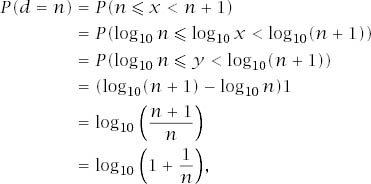
which is Benford’s Law.

The reader may well detect the Weyl Equidistribution Theorem lurking here!

Extending the Law

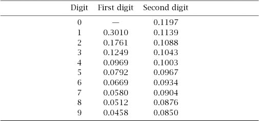
Newcomb’s general arguments in the paper mentioned earlier, which understandably he framed in terms of logarithms, led him to a table, described by the phrase

We thus find the required probabilities of occurrence in the case of the first two significant digits of a natural number to be [as reproduced in table 16.4].

We can see that his first column heralded the Benford Law figures that we have derived: to establish the second we can proceed as follows.

If we isolate the first two significant digits of a number by writing the number as x₁x₂ × 10ⁿ, where 10 x₁x₂ 99, and define the random variable X accordingly, we have

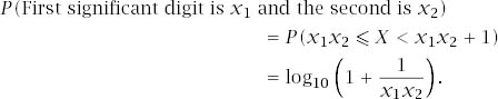
Now observe that

and we have the result

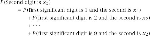
A small computation yields the second column of the table and the reader may wish to pursue matters further to establish the truth of another of his statements in the paper:

In the case of the third figure the probability will be nearly the same for each digit, and for the fourth and following ones the difference will be inappreciable.

Other results can be inferred too. For example, using that standard definition of conditional probability once again,

So, for example, the probability that the second digit of a number is 5 given that its first digit is 6 is , whereas if it started with 9 the probability is .

The most likely start to a number turns out to be 10, with a probability of .

Finally, this has been seen to be more than a theoretical curiosity. Most particularly, Mark Nigrini has pioneered its use in accounting. Quoting from him:

Here are some possible practical applications for Benford’s Law and digital analysis.

• Accounts payable data.

• Estimations in the general ledger.

• The relative size of inventory unit prices among locations.

• Duplicate payments.

• Computer system conversion (for example, old to new system; accounts receivable files).

• Processing inefficiencies due to high quantity/low dollar transactions.

• New combinations of selling prices.

• Customer refunds.

Which is rather more than Newcomb envisaged, to judge by this final quotation from his paper:

It is curious to remark that this law would enable us to decide whether a large collection of independent numerical results were composed of natural numbers or logarithms.