CHAPTER 12: RISK LEVEL
Risk level – the output of the risk equation that we discussed earlier – is a function of impact and likelihood (probability). The final step in the risk assessment exercise is to assess the risk level for each impact and to transfer the details to the corporate asset inventory.
Three levels of risk assessment are usually adequate: low, medium and high. Where the likely impact is low and the probability is also low, then the risk level could be considered very low. Where the impact is at least high and the probability is also at least high, then the risk level might (depending on the design of the risk matrix) be either high or very high.
Every organisation has to decide for itself what it wants to set as the thresholds for categorising each potential impact and from time to time it may be helpful to have four or more risk levels (including one such as minimal) in order to better prioritise actions.
The risk scale
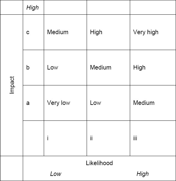
The basic risk scale, which is set out overleaf, plots estimated impact against estimated likelihood.
In this scale, a different category of labels has been applied to both the impact (lower case alphabetic characters) and the likelihood (lower case Roman numerals) scales to indicate low, medium and high. The reason for doing this is to avoid confusion in discussions and communications between members of the risk assessment team and with other parties. For example, a high likelihood (iii) and a high impact (c) identify something that would be very high risk, whereas a medium risk in the table is a function of likelihood (i) and impact (c), or (ii) and (b), or (iii) and (a).

Figure 14: The risk scale
While that is clear, the table only becomes useful when each band has objective criteria applied to it which enable different people in different parts of the organisation to use it on a consistent basis.
The usual way of doing this is to allocate specific ranges to each band. For instance, the impact bands might be:
Impact
c From £1m to £5m (anything in excess of £5m is rejected)
b From £100,000 to £999,999
a From zero to £99,999.
The likelihood bands might be:
Likelihood
i Less than once every year (very infrequent)
ii Between once a month and once a year (often)
iii More than once a month (very often).
These bands enable different people, in different parts of the organisation, to assess risks in a similar way. Automated hacking attacks on an online bank, for instance, would be placed in impact category b (between £100,000 and £999,999) and likelihood category iii (very often); the assessed risk level would therefore be ‘high’. Similarly, manual hack attacks might be placed in impact level c (over £1m) but only at likelihood level ii (often). Intersection of these two lines would also give rise to an assessed risk of ‘high’.
The qualitative methodology has been useful in enabling different threat-vulnerability combinations to be quickly assessed, and for comparative risk assessment decisions to be made – without detailed, faux-accurate calculations as to potential impact.
Both risks fall outside the organisation’s risk tolerance level, and both should be controlled. The organisation’s risk acceptance criteria include the requirement that the cost of control should be in line with the identified potential impact. But how do we determine, in this example, how much to spend on implementation?
Boundary calculations
One approach is to calculate the risk value (risk = impact x likelihood) at the borders of each risk value and for the investment criteria to be as simple as: spend no less than [the lower risk level] and no more than [the higher risk level]. Each level has an upper and a lower boundary, the point at which the risk shifts from being at one level to being at the next. For example, the border values for ‘very low’ in our table would be:
Lower boundary: a (low) x i (low), or 0 x 0, which equals zero.
Upper boundary: a (high) x i (high), or 1 x £99,999, which equals £99,999.
In other words, according to this risk assessment scale, this risk would have an impact that falls somewhere between £0 and £99,999 and the risk treatment decision (if this risk was outside the risk acceptance boundary) would allow no more than £99,999 to be invested in control implementation.
While this appears clear cut, the situation is less clear for those risk levels that occur more than once. For instance, the medium risk level (let’s call it risk 1 in this example) could fall within the ranges of:
Impact high (c) and likelihood low (i), the boundaries of which would be:
Lower boundary: c (low) x i (low), or £1m x 0, which equals 0.
Upper boundary: c (high) x i (high), or £5m x 1, which equals £5m.
The medium risk level also exists at the intersection of impact (b) and likelihood (ii). The boundary calculations (for what we will call risk 2 in this example) would be:
Lower boundary: b (low) x ii (low), or £100,000 x 1, which is £100,000.
Upper boundary: b (high) x ii (high), or £999,999 x 12, which is (about) £12m.
So, a risk (Risk 1), assessed as a medium risk, has a potential impact of between £0 and £5m. Another risk (Risk 2), also assessed as a medium risk, has a potential impact of between £100,000 and £12m. These clearly different impact ranges need to be recognised when developing the organisational risk assessment methodology, and there are three useful ways of responding to them.
• The first is to ensure that the scale you use is sufficiently granular; in real terms, a five-level scale may – for many organisations – provide a more useful basis of assessment.
• The second is for the risk assessment methodology to explicitly recognise that there will be ‘fuzzy areas’ at the boundaries, and for the board to delegate authority to the risk assessor to review and adjust (what we call ‘smoothing’) those individual control decisions that appear to be misaligned as a result of these calculations, to ensure that there is an equivalence of investment.
• The third is to use ‘mid-points’ instead of boundary calculations to provide guidance on control investment. While these calculations do not remove the need to address both points 1 and 2 above, they do reduce the magnitude of the overlap and, therefore, can provide more useful risk assessment guidance.
Mid-point calculations
An alternative, and more helpful, approach is to calculate the mid-points for each range, and to use those calculated numbers to guide investment decisions.
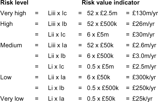
The starting point for this calculation is to identify mid-points (i.e. the points between the upper and lower levels) for each of the risk factors (likelihood and impact). The mid-points for each of the factors in Figure 14, above, would be:

We can then apply these to calculate the mid-point for each of the identified risks, to produce what we call a ‘risk value indicator’. Please note the term ‘indicator’: we are using a qualitative methodology, and this is an indicator to provide guidance.

As these calculations demonstrate, there is a range of risk value indicators for each risk level, even when considering only the mid-point in the corresponding likelihood and impact scales. From an investment perspective, the control investment decision will be to invest an amount approximately the same as the risk value indicator. As guidance goes, the risk assessment team will find this more useful than guidance which is based on boundary calculations. It is well worth remembering here the ‘approximately correct rather than precisely wrong’ mantra.
The organisation’s documented risk acceptance criteria should, if a mid-point calculation is used, include a description of how it is calculated and how the risk value indicator is to be used in risk treatment decisions. The formal risk acceptance criteria should also state that, while it is the mid-points that have been used to demonstrate the different levels of risk and guide control investment decisions, it is the entire level that is either within or outside the acceptance criteria.
