
End-to-End Acoustic Modeling Using Convolutional Neural Networks
Vishal Passricha; Rajesh Kumar Aggarwal National Institute of Technology Kurukshetra, Kurukshetra, India
Abstract
State-of-the-art automatic speech recognition (ASR) systems map speech into its corresponding text. Conventional ASR systems model the speech signal into phones in two steps; feature extraction and classifier training. Traditional ASR systems have been replaced by deep neural network (DNN)-based systems. Today, end-to-end ASRs are gaining in popularity due to simplified model-building processes and the ability to directly map speech into text without predefined alignments. These models are based on data-driven learning methods and competition with complicated ASR models based on DNN and linguistic resources. There are three major types of end-to-end architectures for ASR: Attention-based methods, connectionist temporal classification, and convolutional neural network (CNN)-based direct raw speech model.
This chapter discusses end-to-end acoustic modeling using CNN in detail. CNN establishes the relationship between the raw speech signal and phones in a data-driven manner. Relevant features and classifiers are jointly learned from raw speech. The first convolutional layer automatically learns feature representation. That intermediate representation is more discriminative and further processed by rest convolutional layers. This system performs better than traditional cepstral feature–based systems but uses a high number of parameters. The performance of the system is evaluated for TIMIT and claimed better performance than MFCC feature-based GMM/HMM (Gaussian mixture model/hidden Markov model) model.
Keywords
Automatic speech recognition (ASR); Attention-based model; Connectionist temporal classification; Convolutional neural network (CNN); End-to-end model; Raw speech signal
2.1 Introduction
An automatic speech recognition (ASR) system has two important tasks—phoneme recognition and whole word decoding. In ASR, the relationship between the speech signal and phones are established in three steps [1]. First, useful features are extracted from the speech signal on the basis of prior knowledge. This phase is known as information selection, dimensionality reduction, or feature extraction phase. In this, the dimensionality of the speech signal is reduced by selecting the information based on task-specific knowledge. Highly specialized features like MFCC (Mel-frequency cepstral coefficient) [2] and PLP (perceptual linear prediction) [3] are the preferred choices in traditional ASR systems. Next, generative models like Gaussian mixture model (GMM), hidden Markov model (HMM), or discriminative models like artificial neural networks (ANNs), deep neural networks (DNNs), and convolutional neural networks (CNNs) estimate the likelihood of each phoneme. This step is known as acoustic modeling. Finally, word sequence is recognized using dynamic programming technique. This step is decision making, it integrates the acoustic model, lexical and language model to decode the text utterance. Deep learning systems can map the acoustic features into the spoken phonemes directly. A sequence of the phoneme is easily generated from the frames using frame level classification.
Another side, end-to-end systems perform acoustic frames to phone mapping in one step only. End-to-end training means all the modules are learned simultaneously. Advanced deep learning methods facilitate the training of the ASR system in an end-to-end manner. They can also train ASR system directly with raw signals, that is, without hand-crafted features. Therefore, the ASR paradigm is shifting from cepstral features like MFCC, PLP to discriminative features learned directly from raw speech. The end-to-end model may take a raw speech signal as input and generates phoneme class conditional probabilities as output. The three major types of end-to-end architectures for ASR are attention-based method, connectionist temporal classification (CTC), and CNN-based direct raw speech model. End-to-end trained systems are gaining popularity in speech signal to word sequence [4–9].
Attention-based models directly transcribe the speech into phonemes by jointly training an acoustic model, language model, and alignment mechanism. Attention-based encoder-decoder uses the recurrent neural network (RNN) to perform sequence-to-sequence mapping without any predefined alignment. In this model, the input sequence is first transformed into a fixed-length vector representation and then the decoder maps this fixed-length vector into the output sequence. Attention-based encoder-decoder is capable of learning the mapping between variable-length input and output sequences. Chorowski and Jaitly [10] proposed speaker independent sequence-to-sequence model that achieved 10.6% word error rate (WER) without separate language models and 6.7% WER with a trigram language model for Wall Street Journal dataset. In attention-based systems, the alignment between the acoustic frames and recognized symbols is performed by the attention mechanism, whereas the CTC model uses conditional independence assumptions to solve sequential problems by dynamic programming efficiently. Attention model has shown high performance over the CTC approach because it uses the history of the target character without any conditional independence assumptions. Soltau et al. [11] performed context-dependent phoneme recognition by training the CTC-based model on YouTube video caption task. Sequence-to-sequence models lack behind 13%–35% than baseline systems. Graves et al. [12] trained the end-to-end model on CTC criterion without applying a frame-level alignment. A sequence-to-sequence model simplified the ASR problem by learning and optimizing the neural network for an acoustic model, pronunciation model, and language model [5, 7, 9, 13]. These models also work as multi-dialects systems because they are jointly modeled across dialects. Li and others [14] trained a single sequence to sequence model for multi-dialect speech recognition and achieved a similar performance as another sequence-to-sequence model for single dialect tasks.
Another side, the CNN-based acoustic model is proposed by Palaz et al. [15–17] which processes the raw speech directly as input. This model consists of two stages: Feature learning stage, that is, several convolutional layers and classifier stage, that is, fully connected layers. Both the stages are learned jointly by minimizing a cost function based on relative entropy. In this model, the features are extracted by the filters at the first convolutional layer and processed between the first and second convolutional layer. In the classifier stage, learned features are classified by fully connected layers and a softmax layer, that is, model the relation between features and phoneme. This approach claims comparable or better performance than traditional cepstral feature-based system followed by ANN trained for phoneme recognition on TIMIT dataset.
CNN has three advanced features over DNN i.e., convolutional filters, pooling, and weight sharing. Pooling operator is applied to extract lower & higher level features. The key features of pooling are achieving compact representation and more robustness to noise and clutter. Various pooling strategies are found obscure by several compounding factors. Various pooling strategies like max pooling, average pooling, stochastic pooling, Lp pooling, etc. have their own advantages and disadvantages. It is always critical to understand and select the best pooling technique. In this chapter, we compare various pooling strategies for end-to-end CNN-based direct raw speech model. We further explore the effects of nonlinearity of fully connected layers on the recognition rate.
This chapter is organized as follows: In Section 2.2, the work performed in the field of ASR is discussed with the name of related work. Section 2.3 covers the various architectures of ASR. Section 2.4 presents the brief introduction about CNN. Section 2.5 explains the CNN-based direct raw speech recognition model. In Section 2.6, the available experiment and their results are shown. Finally, Section 2.7 concludes this chapter with a brief discussion.
2.2 Related Work
A traditional ASR system leveraged the GMM/HMM paradigm for acoustic modeling. GMM efficiently processes the vectors of input features and estimates emission probabilities for each HMM state. HMM efficiently normalizes the temporal variability present in the speech signal. The combination of HMM and the language model is used to estimate the most likely sequence of phones. The discriminative objective functions, that is, maximum mutual information, minimum classification error, minimum phone error, and minimum word error (MWE) are used to improve the recognition rate of the system by the discriminative training methods [18]. However, GMM has a shortcoming because it shows an inability to model the data that lie on or near a nonlinear manifold in the dataspace [19]. Therefore its performance degrades in the presence of noise. On the other hand, ANNs can learn much better models of data that lay in the noisy conditions. DNNs as acoustic models tremendously improved the performance of ASR systems [19–21]. Generally, discriminative power of DNNs is used for phoneme recognition and for decoding task, HMM is the preferred choice. DNNs have many hidden layers with a large number of nonlinear units and a very large output layer. The benefit of this large output layer is that it accommodates a large number of HMM states that arise when each phone is modeled by a number of different “triphone” HMMs, which take into account the phones on either side. DNN architecture has densely connected layers. Therefore such architectures are more prone to overfitting. Secondly, features that have the local correlations become difficult to learn by such architectures. On the other hand, in [22], speech frames are classified into clustered context-dependent states using DNNs. In [23, 24], GMM-free DNN training process is proposed by the researchers. However, GMM-free process demands iterative procedures like decision trees and generating forced alignments. DNN-based acoustic models are gaining popularity in large vocabulary speech recognition tasks [19], but components like HMM and an n-gram language model are the same as in their predecessors.
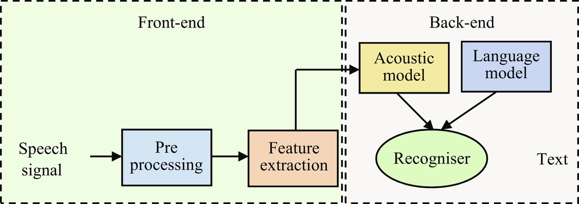
GMM- or DNN-based ASR systems perform the task in three steps: feature extraction, classification, and decoding. It is shown in Fig. 2.1. Firstly, the short-term signal st are processed at time ‘t’ to extract the features xt. These features are provided as input to GMM or DNN acoustic model which estimates the class conditional probabilities Pe(i | xi) for each phone class i ∈ {1, …, I}. The emission probabilities are as follows:
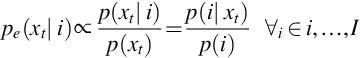
The prior class probability p(i) is computed by counting on the training set.
DNN is a feed-forward NN containing multiple hidden layers with a large number of hidden units. DNNs are trained using the back-propagation methods, then they are discriminatively fine-tuned for reducing the gap between desired output and actual output. DNN/HMM-based hybrid systems are the effective models that use a triphone HMM model and an n-gram language model [19, 25]. Traditional DNN/HMM hybrid systems have several independent components that are trained separately like an acoustic model, pronunciation model, and language model. In the hybrid model, the speech recognition task is factorized into several independent subtasks. Each subtask is independently handled by a separate module, which simplifies the objective. The classification task is much simpler in HMM-based models as compared to classifying the set of variable length sequences directly. This is because sequence classification with variable length requires sequence padding of data and some advanced models like long short-term memory (LSTM), bidirectional long short-term memory (BLSTM), etc. Fig. 2.2 shows the hybrid DNN/HMM phoneme recognition model.

On the other side, researchers proposed end-to-end ASR systems that directly map the speech into labels without any intermediate components. As an advancement in deep learning, it became possible to train the system in an end-to-end fashion. The high success rate of deep learning methods in vision task motivates the researchers to focus on the classifier step for speech recognition. Such architectures are called deep because they are composed of many layers as compared to classical shallow systems. The main goal of an end-to-end ASR system is to simplify the conventional module-based ASR system into a single Deep Learning framework. In earlier systems, divide and conquer approaches are used to optimize each step independently whereas Deep Learning approaches have a single architecture that leads to the more optimal system. End-to-end speech recognition systems directly map the speech into text without requiring predefined alignment between acoustic frame and characters [5–7, 9, 26–30]. These systems are generally divided into three broad categories: Attention-based model [6, 7, 28, 29], CTC [5, 12, 26, 27], and CNN-based direct raw speech method [15–17, 31]. All these models can address the problem of variable-length input and output sequences.
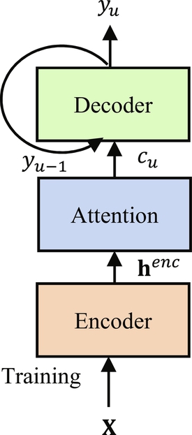
Attention-based models are gaining popularity in a variety of tasks like handwriting synthesis [32], machine translation [33], and visual object classification [34]. Attention-based models directly map the acoustic frame into character sequences. However, this model differs from other machine translation tasks by requesting much longer input sequences. This model generates a character based on the inputs and history of the target character. The attention-based models use encoder-decoder architecture to perform the sequence mapping from speech feature sequences to text as shown in Fig. 2.3. Its extension, that is, attention-based recurrent networks have also been successfully applied to speech recognition. In the noisy environment, these models’ results are poor because noise easily corrupts the estimated alignment. Another issue with this model is that it is hard to train from scratch due to misalignment on longer input sequences. Sequence-to-sequence networks have also achieved many breakthroughs in speech recognition [6, 7, 29]. They can be divided into three modules: an encoding module that transforms sequences; an attention module that estimates the alignment between the hidden vector and targets; and the decoding module that generates the output sequence. It replaces the complex data processing pipelines with a single neural network trained in end-to-end fashion. It is directly trained by discriminative training methods to maximize the probability of observing desired outputs conditioned on the inputs. The discriminative training is a different way of training that raises the performance of the system by focusing on most informative features. It also overcomes the risk of overfitting, so it is currently gaining high popularity. Therefore to develop a successful sequence-to-sequence model, the understanding and preventing limitations are required.
End-to-end trainable speech recognition systems are an important application of attention-based models. The decoder network computes a matching score between hidden states generated by the acoustic encoder network at each input time. It processes its hidden states to form a temporal alignment distribution. This matching score is used to estimate the corresponding encoder states. The difficulty of an attention-based mechanism in speech recognition is that the feature inputs and corresponding letter outputs generally proceed in the same order with only small deviations within word. However, the different length of input and output sequences make it more difficult to track the alignment. The advantage of an attention-based mechanism is that any conditional independence assumptions (Markov assumption) are not required in this mechanism. Attention-based approach replaces the HMM with RNN to perform the sequence prediction (Fig. 2.4). The attention mechanism automatically learns alignment between the input features and desired character sequence.
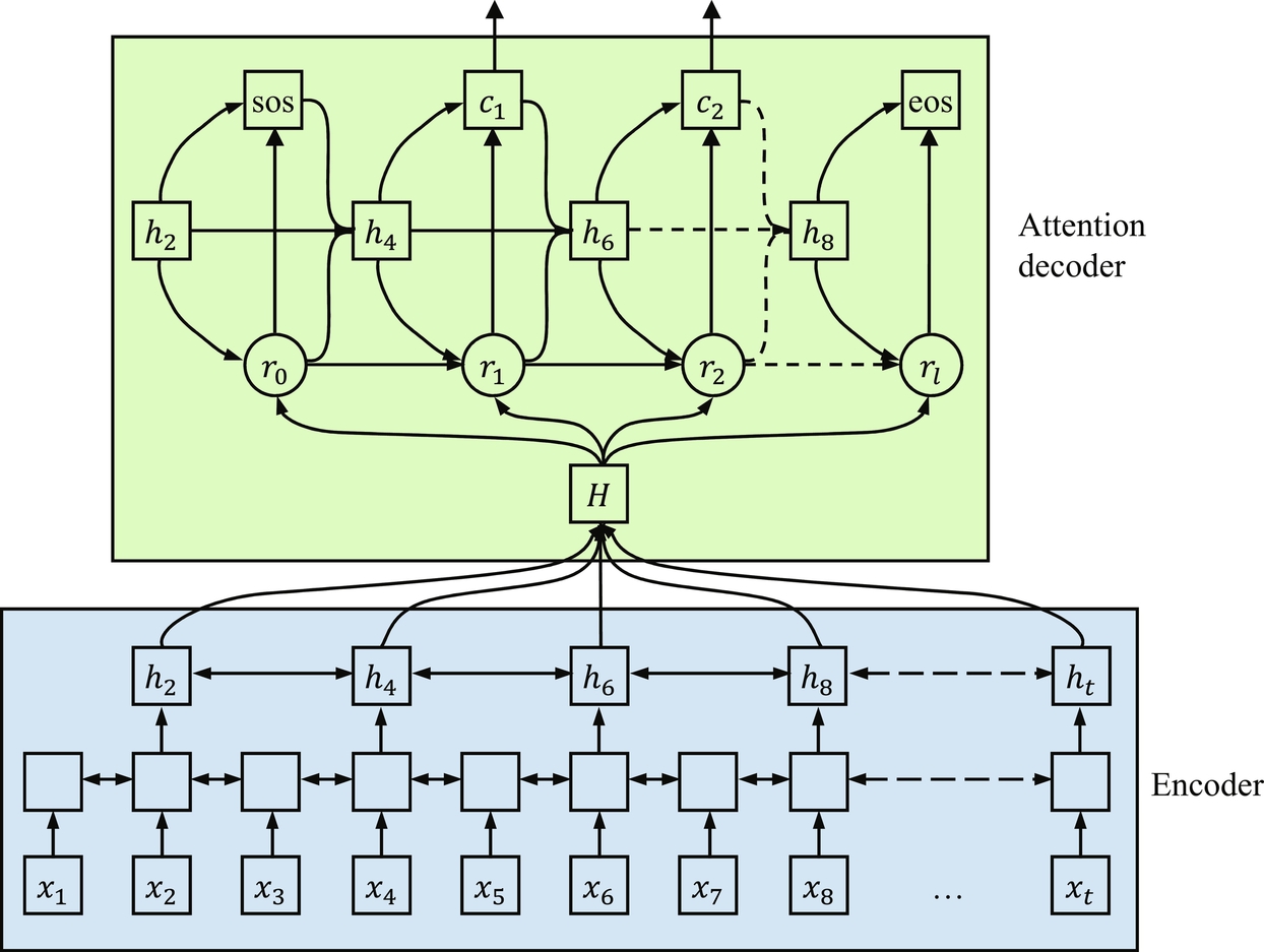
CTC techniques infer the speech-label alignment automatically. CTC [12] was developed for decoding the language. Hannun et al. [26] used it for decoding purposes in Baidu’s deep speech network. CTC uses dynamic programming [5] for efficient computation of a strictly monotonic alignment. However, graph-based decoding and a language model are required for it. CTC approaches use RNN for feature extraction [33]. Graves et al. [35] used its objective function in BLSTM system. This model successfully arranges all possible alignments between input and output sequences during model training.
Two different versions of beam search are adopted by [5, 36] for decoding CTC models. Fig. 2.5 shows the working architecture of the CTC model. In this, noisy and noninformative frames are discarded by the introduction of the blank label, which results in the optimal output sequence. CTC uses intermediate label representation to identify the blank labels, that is, no output labels. CTC-based NN model shows a high recognition rate for both phoneme recognition [4] and large vocabulary continuous speech recognition (LVCSR) [5, 36]. CTC trained neural network with language model offers excellent results [26].

In Fig. 2.5, {x1, x2, …, xt} represents our input sequence, {h2, h4, …, ht} represents the high-level features, and {Y1, Y2, …} represents the letter sequence generated by the CTC decoder. End-to-end ASR systems perform well and achieve good results, yet they face two major challenges. First, how to incorporate lexicons and language models into decoding. However, [5, 36] has incorporated lexicons for searching paths. Second, there is no shared experimental platform for the purpose of the benchmark. End-to-end systems differ from the traditional systems in both aspects, model architecture as well as decoding methods. Some efforts were also made to model the raw speech signal with little or no preprocessing [37]. Earlier, Jaitly and Hinton [37] used restricted Boltzmann machines, Tüske et al. [38] used DNN and Sainath et al. [39] used the combination of convolutional, long short-term memory with fully connected DNN to process the raw waveforms. Although, results did not meet the previously available results. The NN architectures with local connections and shared weights are called CNN [40]. Palaz et al. [16] showed in his study that CNN could calculate the class conditional probabilities from the raw speech signal as direct input. Therefore CNNs are the preferred choice to learn features from the raw speech. There are two stages of learned features process. Features are learned by the filters at the first convolutional layer, then learned features are modeled by second and higher level convolutional layers. An end-to-end phoneme sequence recognizer directly processes the raw speech signal as input and produces a phoneme sequence. This end-to-end system is composed of two parts: CNNs and conditional random field (CRF). CNN is used to perform the feature learning and classification, and CRFs are used for the decoding stage. CRF, ANN, multilayer perceptron etc. have been successfully used as decoder. The results on TIMIT phone recognition task also confirm that the system effectively learns the features from raw speech and performs better than traditional systems that take cepstral features as input [41]. This model also produced good results for LVCSR [17]. Table 2.1 shows the comparison of different end-to-end speech recognition model in the form of WER.
Table 2.1
| Model | Clean | Noisy | Numeric Values Only | ||
|---|---|---|---|---|---|
| Isolated Words | Continuous Speech | Isolated Words | Continuous Speech | ||
| Baseline unidirectional context-dependent phoneme | 6.4 | 9.9 | 8.7 | 14.6 | 11.4 |
| Baseline bidirectional context-dependent phoneme | 5.4 | 8.6 | 6.9 | _ | 11.4 |
| End-to-end systems | |||||
| CTC grapheme | 39.4 | 53.4 | _ | _ | _ |
| RNN transducer | 6.6 | 12.8 | 8.5 | 22.0 | 9.9 |
| RNN transducer with attention | 6.5 | 12.5 | 8.4 | 21.5 | 9.7 |
| Attention 1-layer decoder | 6.6 | 11.7 | 8.7 | 20.6 | 9.0 |
| Attention 2-layer decoder | 6.3 | 11.2 | 8.1 | 19.7 | 8.7 |

2.3 Various Architecture of ASR
In this section, a brief review on conventional GMM/DNN ASR, attention-based end-to-end ASR, and CTC is given.
2.3.1 GMM/DNN
ASR system performs sequence mapping of T-length speech sequence features, X = {Xt ∈ ℝD | t = 1, …, T}, into an N-length word sequence, W = {wn ∈ υ | n = 1, …, N} where Xt represents the D-dimensional speech feature vector at frame t, and wn represents the word at position n in the vocabulary υ.
The ASR problem is formulated within the Bayesian framework. In this method, an utterance is represented by some sequence of acoustic feature vector X, derived from the underlying sequence of words W, and the recognition system needs to find the most likely word sequence, given below [42]:
In Eq. (2.2), the argument of p(W | X), that is, the word sequence W is found which shows the maximum probability for given feature vector, X. Using Bayes’ rule, it can be written as:
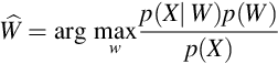
In Eq. (2.3), the denominator p(X) is ignored as it is constant with respect to W. Therefore,
where p(X | W) represents the likelihood of the feature vector X and it is evaluated with the help of an acoustic model. p(W) represents the prior knowledge, that is, a priori probability about the sequence of words W and it is determined by the language model. However, current ASR systems are based on a hybrid HMM/DNN [43], that is also calculated using Bayes’ theorem and introduces the HMM state sequence S, to factorize p(W | X) into the following three distributions:
where p(X | S), p(S | W), and p(W) represent acoustic, lexicon, and language models respectively. υ⁎ represents the all possible word sequence. Eq. (2.6) is changed into Eq. (2.7) by a conditional independence assumption. Note: It is a reasonable assumption to simplify the dependency of the acoustic model.
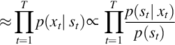
- (a) Acoustic models p(X | S): p(X | S) can be further factorized using a probabilistic chain rule and Markov assumption as follows:
In Eq. (2.9), framewise likelihood function p(xt | st) is changed into the framewise posterior distribution , which is computed using DNN classifiers by pseudo-likelihood trick [43]. In Eq. (2.9), the Markov assumption is too strong. Therefore the contexts of input and hidden states are not considered. This issue can be resolved using either the RNNs or DNNs with long context features. A framewise state alignment is required to train the framewise posterior, which is offered by an HMM/GMM system.
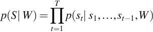
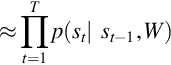
 - (b) Lexicon model p(S | W): p(S | W) can be further factorized using a probabilistic chain rule and Markov assumption (first order) as follows:
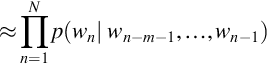
An HMM state transition represents this probability. A pronunciation dictionary performs the conversion from w to HMM states through phoneme representation. - (c) Language model p(W): Similarly, p(W) can be factorized using a probabilistic chain rule and Markov assumption ((m − 1)th order) as an m-gram model, that is,
The issue of Markov assumption is addressed using RNN language model (RNNLM) [44], but it increases the complexity of the decoding process. The combination of RNNLMs and m-gram language model is generally used and it works on a rescoring technique.


2.3.2 Attention Mechanism
The approaches based on attention mechanism does not make any Markov assumptions. It directly finds the posterior probability p(C | X), on the basis of a probabilistic chain rule.
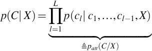
where patt(C | X) represents an attention-based objective function. C represents the L-length letter sequence. p(cl | c1, …, cl − 1, X) is obtained by

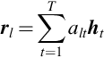
Eq. (2.15) represents the encoder and Eq. (2.18) represents the decoder networks. alt represents the soft alignment of the hidden vector, ht. It is also known as attention weight. Here, rl represents the weighted letter-wise hidden vector that is computed by weighted summation of hidden vectors. Content-based attention mechanism with or without convolutional features are represented by ContentAttention(⋅) and LocationAttention(⋅), respectively.
- (a) Encoder network: The input speech feature sequence X is converted into a framewise hidden vector, ht using Eq. (2.15). The preferred choice for an encoder network is BLSTM that is,
It is to be noted that the computational complexity of the encoder network is reduced by subsampling the inputs [6, 7]. - (b) Content-based attention mechanism: ContentAttention(⋅) is shown as
g represents a learnable parameter. represents a T-dimensional vector. tanh(⋅) and Lin(⋅) represent the hyperbolic tangent activation function, and linear layer with learnable matrix parameters respectively.
 - (c) Location-aware attention mechanism: It is an extended version of content-based attention mechanism to deal with the location-aware attention (i.e., convolution). We know that
 . If
. If  is replaced in Eq. (2.16), then LocationAttention(⋅) is represented as follows:
Here, ⁎ denotes 1-D convolution along the input feature axis, t, with the convolution parameter, , to produce the set of T features
  . LinB(⋅) represents the linear layer with learnable matrix parameters with bias vector parameters.
 - (d) Decoder network: The decoder network is an RNN that is conditioned on previous output Cl − 1 and hidden vector ql − 1. LSTM is the preferred choice of RNN that is represented as follows:
LSTMl(⋅) represents uniconditional LSTM that generates hidden vector ql as output.
rl represents the concatenated vector of the letter-wise hidden vector, cl − 1 represents the output of the previous layer which is taken as input. - (e) Objective function: The training objective of the attention model is computed from the sequence posterior
where cl⁎ represents the ground truth of the previous characters. The attention-based approach is a combination of letter-wise objectives based on multiclass classification with the conditional ground truth history in each output l, and does not fully consider a sequence-level objective, as pointed out by [6].

2.3.3 Connectionist Temporal Classification
The CTC formulation is also based on Bayes’ decision theory. CTC formulation uses letter sequence C with blank symbol to denote the letter boundary to handle the repetition of letter symbols. An augmented letter sequence
In C′, cl′ represents letter symbol produced. ![]() represents the set of distinct letters. l is the number between 1 and 2L + 1 that decides the produced symbol is blank or letter symbol. cl′ is always “〈b〉” and letter when l is an odd and an even number, respectively. Similar to DNN/HMM model, framewise letter sequence with an additional blank symbol
represents the set of distinct letters. l is the number between 1 and 2L + 1 that decides the produced symbol is blank or letter symbol. cl′ is always “〈b〉” and letter when l is an odd and an even number, respectively. Similar to DNN/HMM model, framewise letter sequence with an additional blank symbol
is also introduced. The posterior distribution, p(C | X), can be factorized as
Same as Eq. (2.7), CTC also uses Markov assumption, that is, p(C | Z, X) ≈ p(C | Z) to simplify the dependency of the CTC acoustic model, p(Z | X), and CTC letter model, p(C | Z).
- (a) CTC acoustic model: Same as DNN/HMM acoustic model, p(Z | X) can be further factorized using a probabilistic chain rule and Markov assumption as follows:

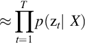
The framewise posterior distribution, p(zt | X) is computed from all inputs, X, and it is directly modeled using BLSTM [35, 45].
BLSTMt(⋅) takes full input sequence as input and produces hidden vector (ht) at t. Where Softmax(⋅) represents the softmax activation function. LinB(⋅) is used to convert the hidden vector, ht, to a ![]() dimensional vector with learnable matrix and bias vector parameter.
dimensional vector with learnable matrix and bias vector parameter.
- (b) CTC letter model: By applying, Bayes’ decision theory probabilistic chain rule, and Markov assumption, p(C | Z ) can be written as
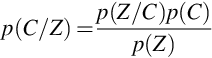

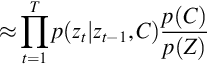
where p(zt | zt − 1, C) represents state transition probability. p(C) represents a letter-based language model, and p(Z) represents the state prior probability. CTC architecture incorporates letter-based language model. CTC architecture can also incorporate a word-based language model by using a letter-to-word finite state transducer during decoding [27]. The CTC has the monotonic alignment property. That is, when zt − 1 = c′m, then zt = cl′ where l ≥ m.
Monotonic alignment property is an important constraint for speech recognition, so ASR sequence-to-sequence mapping should follow the monotonic alignment. This property is also satisfied by HMM/DNN.
- (c) Objective function: The posterior, p(C | X) is represented as
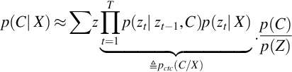
Viterbi method and forward–backward algorithm are dynamic programming algorithms, which are used to efficiently compute the summation over all possible Z. CTC objective function pCTC(C | X) is designed by excluding the p(C)/p(Z) from Eq. (2.23).
The CTC formulation is also the same as HMM/DNN. The minute difference is that Bayes’ rule is applied to p(C | Z) instead of p(W | X). It has also three distribution components like HMM/DNN that is, framewise posterior distribution, p(zt | X), transition probability, p(zt | zt − 1, C), and letter model, p(C). It also uses the Markov assumption. It does not fully utilize the benefit of end-to-end ASR but its character output representation still possesses the end-to-end benefits.
2.4 Convolutional Neural Networks
CNNs are the popular variants of deep learning that are widely adopted in ASR systems. CNNs have many attractive advancements, that is, weight sharing, convolutional filters, and pooling. Therefore CNNs have achieved an impressive performance in ASR. CNNs are composed of multiple convolutional layers. Fig. 2.6 shows the architecture of CNN for speech recognition. LeCun and Bengio [46] describe the three main sublayers of CNN layer, that is, convolution, pooling, and nonlinearity. Each one of the concepts has the potential to boost speech recognition performance.

Locality, weight-sharing, and pooling are the key properties of CNNs that have potential to improve speech recognition performance. Locality offers more robustness against nonwhite noise where some bands are cleaner than the others. The reason is that good features can be computed locally from the cleaner parts of the spectrum and only a smaller number of features are affected by the noise. By this, higher layers of the network get better chance to handle the noise by combining higher level features computed from each frequency band. Locality reduces the number of weights to be learned. Convolutional filters or local filters are imposed on a subset region of the previous layer to capture a specific kind of local patterns known as structural locality. Different phonemes have different energy concentrations in different local bands along the frequency axis. The process of distinguishing different phonemes becomes critical due to these local energy concentrations. These small local energy concentrations also cause the problem of temporal evaluation. These small local energy concentrations of the input are processed by a set of local filters that are applied by a convolutional layer. Local filters are also effective against ambient noises. Weight sharing improves the model robustness by reducing overfitting. It also reduces the number of network weights. The differences in vocal tract lengths among different speaker cause the frequency shifts in speech signals. Weight-sharing carefully handles these frequency shifts, whereas other models like GMMs or DNNs are failed to effectively handle these shifts. In CNN, input is an image of mel-log filter energies visualized as spectrogram. Therefore, CNN ran a small-sized window over the input image; both training and testing time. By this process, the weights of the network learn from the various features of the input data. The properties of the speech signal vary over different frequency bands. Therefore, separate sets of weights for different frequency bands may be more fruitful. This process is known as limited weight sharing. In full weight sharing scheme, convolutional units attached to the same pooling unit share the same convolutional weight. These convolutional units share their weights to compute comparable features.
CNN consists of a special network structure, that is, alternate convolutional and pooling layers. Deep CNNs set a new milestone by achieving approximate human level performance through advanced architectures and optimized training [47]. CNNs use nonlinear function to directly process the low-level data. CNNs are capable of learning high-level features with high complexity and abstraction. Maxout is a widely used nonlinearity that has shown its effectiveness in ASR tasks [48, 49]. Pooling is the heart of CNNs which reduces the dimensionality of a feature map. Pooling causes the minimal differences in the feature extracted because different locations are pooled together. Max pooling is helpful in handling slight shifts in the input pattern along the frequency axis.
Pooling is an important concept that transforms the joint feature representation into the valuable information by keeping the useful information and eliminating insignificant information. Small frequency shifts that are common in speech signal are efficiently handled using pooling. Pooling also helps in reducing the spectral variance present in the input speech. It maps the input from p adjacent units into the output by applying a special function. After the element-wise nonlinearities, the features are passed through pooling layer. This layer executes the down-sampling on the feature maps coming from the previous layer and produces the new feature maps with a condensed resolution.
The main aim of CNN is to discover local structure in input data. CNN successfully reduces the spectral variations, and it can adequately model the spectral correlations in acoustic features. Earlier the convolution was applied only on frequency axis which made the ASR system more robust against variations generated from different speaking style and speaker [22, 50, 51]. Later, Toth [52] applied convolution along the time axis. Unfortunately, the improvement was negligible. Therefore convolution is generally applied only along the frequency axis because shift-invariance in frequency is more important than shift-invariance in time [51, 53, 54].
CNNs have the capabilities to model temporal correlations with adaptive content information. Therefore they can perform any sequence-to-sequence mapping with great accuracy [55]. CNN layers generate features for succeeding layers that classify them into corresponding classes. The HMMs state emission probability density function is calculated by dividing the state posterior derived from CNNs by the prior probability of the consider state calculated from the training data. The CNN consists of a few sets of convolution and pooling layers. Pooling is generally applied along the frequency domain. Finally, fully connected layers combine inputs from all the positions into a 1-D feature vector. Hence, high-level reasoning is applied on invariant features and then supplied to the softmax, that is, the final layer of the architecture. Finally, the softmax activation layer classifies the overall inputs.
2.4.1 Type of Pooling
CNNs are successfully adopted in many speech recognition tasks and are setting new records. Alternate convolution and pooling layers are followed in CNN architecture, and in last, fully connected layers are used. Pooling is a key-step in CNN-based ASR systems that reduces the dimensionality of the feature maps. Pooling combines a set of values into a smaller number of values. Stride represents the size of pooling, that is, the reduction in dimension of the feature map.
Pooling operators provide a form of spatial transformation invariance, as well as reduce the computational complexity for upper layers by eliminating some connections between convolutional layers. Pooling extracts the output from several regions and combines them. It maps the input from p adjacent units into the output by applying a special function. This layer executes the down-sampling on the feature maps coming from the previous layer and produces the new feature maps with a condensed resolution. This layer drastically reduces the spatial dimension of input. It serves two main purposes. First, it reduces the number of parameters or weight by 65%, thus lessening the computational cost. Second, it controls the overfitting. This term refers to when a model is so tuned to the training examples. An ideal pooling method is expected to extract only useful information, and discard irrelevant details. This section covers earlier proposed pooling methods that have been successfully applied in CNNs.
Researchers have proposed many pooling strategies, and in beginning average and max pooling were popular choice [51, 56]. Max and average pooling are deterministic, that is, extract the maximum activation in each pooling region and took the average of all activations in each pooling region, respectively. Average pooling takes all the activations in a pooling region into consideration with equal contributions. This may downplay high activations since many low activations are also included. Lp pooling [57] and stochastic pooling [58] are alternate pooling strategies that address this problem. Bruna et al. [57] claim that the generalization offered by Lp pooling is better than max pooling.
Stochastic pooling selects from a few specific locations (those with strong responses), rather than all possible locations in the region. It forms multinomial distribution [59] by the activations and uses it to select the activation within the pooling region. It uses the stochastic process, hence it is known as stochastic pooling. Mixed pooling [60] is a hybrid of max and average pooling. It can switch between max pooling and average pooling by parameter λ. It takes the advantages of both pooling but both are deterministic in nature, hence it is also deterministic in nature. Multiscale order pooling is applied to improve the invariance of CNNs [61]. Spectral pooling is an advance pooling strategy that crops the features from the input stream [62]. It overcomes the problem of sharp reduction in dimensionality.
2.4.1.1 Max Pooling
The most popular strategy for CNNs is max pooling, which picks only the maximum activation and discards all other units from the pooling region [22]. The function for max pooling is given in Eq. (2.40).
where Rj is a pooling region and {a1, …, a∣ Rj ∣} is a set of activations. Zeiler and Fergus [58] have shown in their experiments that overfitting of the training data is a major problem with max pooling.
2.4.1.2 Average Pooling
Maximum activation of the filter template for each region is selected by the max pooling. However, other activations in the same pooling region are ignored, this should be taken into account. Instead of always extracting maximum activation from each pooling region as max pooling does, the average pooling takes the arithmetic mean of the element in each pooling region. The function for average pooling is given in Eq. (2.41).

The drawback of average pooling is that all the elements in a pooling region are considered, even if many have low magnitude. It weighs down the strong activations because it combines many sparse elements on average.
2.4.1.3 Stochastic Pooling
Inspired by the dropout [63], Zeiler and Fergus [58] proposed the idea of stochastic pooling. In max pooling, the maximum activation is picked from each pooling region. Whereas the areas of high activation are weighed down by areas of low activation in average pooling because all elements in the pooling region are examined, and their average is taken. It is a major problem with average pooling. The issues of max and average pooling are addressed using stochastic pooling. Stochastic pooling applies multinomial distribution [59] to randomly pick the value. It includes the nonmaximal activations of feature maps. In stochastic pooling, first, the probabilities p is computed for each region j by normalizing the activations within the regions, as given in Eq. (2.42).

These probabilities create a multinomial distribution that is used to select location l, and corresponding pooled activation al is selected based on p. Multinomial distribution selects a location l within the region:
In other words, the activations are selected randomly based on the probabilities calculated by multinomial distribution. Stochastic pooling prohibits overfitting because of the stochastic component. The advantages of max pooling are also found in the stochastic pooling because there’s a likelihood of maximum values and a minimal chance of low values. It also utilizes nonmaximal activations. The procedure is shown in Fig. 2.7.
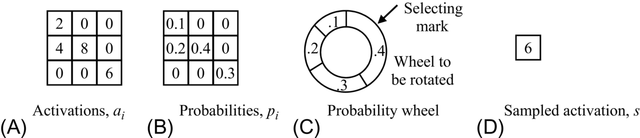
Stochastic pooling represents multinomial distributions of activations within the region, hence the selected element may not be the largest element. It gives high chances to stronger activations and suppresses the weaker activations.
2.4.1.4 Lp Pooling
Sermanet et al. [64] proposed the concept of Lp pooling and claimed that its generalization ability is better than max pooling. In this pooling, a weighted average of inputs is taken in the pooling region. It is shown mathematically below
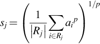
where sj represents the output of the pooling operator at location j, ai is the feature value at location i within the pooling region Rj. The value of p varies between 1 and ∞. When p = 1, Lp operator behaves as average pooling and at p = ∞, it leads to max pooling. For Lp pooling, p > 1 is examined as a trade-off between average and max pooling.
2.4.1.5 Mixed Pooling
Max pooling extracts only the maximum activation, whereas average pooling weighs down the activation by combining the nonmaximal activations. To overcome this problem, Yu et al. [60] proposed a hybrid approach by combining the average pooling and max pooling. This approach is based on Dropout [63] and Dropconnect [65]. Mixed pooling can be represented as
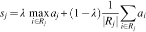
where λ decides the choice of using either max pooling or average pooling. The value of λ is selected randomly in either 0 or 1. When λ = 0, it behaves like average pooling and when λ = 1, it works like max pooling. The value of λ should be recorded during forward-propagation then backpropagation is performed according to the value of λ. Yu et al. [60] showed its superiority over max and average pooling by performing image classification on three datasets.
2.4.1.6 Multiscale Orderless Pooling
Multiscale orderless pooling (MOP) was proposed by Gong et al. [61]. This pooling scheme improves the invariance of CNNs without affecting their discriminative power. MOP processes both whole signal and local patches to extract the deep activation features. The activation features of the whole signal are captured for global spatial layout information and, local patches are captured for more local, fine-grained details of the signal as well as enhancing invariance. Vectors of locally aggregated descriptors encoding [66] is used to aggregate the activation features from local patches. Global spatial activation features and local patch activation features are concatenated using Karhunen-Loeve transformation [67] to obtain the new signal representation.
2.4.1.7 Spectral Pooling
Rippel et al. [62] introduced a new pooling scheme by including the idea of dimensionality reduction by cropping the representation of input in the frequency domain. Let x ∈ Rm × m be an input feature map and h × w be the desired dimensions of the output feature map. First, discrete Fourier transform (DFT) [68] is applied on the input feature map, then h × w size submatrix of frequency representation is cropped from the center. Lastly, inverse DFT is applied on h × w submatrix to convert it into spatial domain again. Spectral pooling preserves the most information for the same output dimensionality by tuning the resolution of input precisely to match the desired output dimensionality compared to max pooling. Spectral pooling does not suffer from the sharp reduction in output dimensionality because the stride-based pooling strategy reduces the dimensionality by at least 75% as a function of stride, and it is not the stride-based pooling method. This process is known as low-pass filtering, which exploits the nonuniformity of the spectral density of the data with respect to frequency. It overcomes the problem of sharp reduction in output map dimensionality. The key idea behind spectral pooling is matrix truncation, which reduces its computation cost in CNNs by employing fast Fourier transformation for convolutional kernels [69].
2.4.2 Types of Nonlinear Functions
This section presents the brief idea about different nonlinear functions that are successfully used in various vision tasks with a remarkable result.
2.4.2.1 Sigmoid Neurons
For acoustic modeling, the standard sigmoid is preferred choice. Fixed function shapes and no adaptive parameters are its strengths. The function of the Sigmoid family is thoroughly explored for many ASR tasks.

f(α) is the logistic function and θ, γ, and η are known as the learnable parameters. Eq. (2.45) denotes the p-sigmoid(η, γ, θ).
In the p-sigmoid function, the curve f(α) have different effects of η, γ, and θ. Among the three parameters, the curve f(α) is highly changed by η because it scales linearly. The value of f(α) that is, ∣ f(α)∣ is always less than or equal to ∣ η ∣. η can be any real number. If η < 0, the hidden unit makes a negative contribution, if η = 0, the hidden unit is disabled, and if η > 0, the hidden unit makes a positive contribution that can be seen as a case of linear hidden unit contributions [70, 71]. If γ ⟶ 0, then f(α) is similar to input around 0. The horizontal difference to f(α) is managed using parameter θ. If γ ≠ 0, then ![]() is the x-value of the mid-point.
is the x-value of the mid-point.
2.4.2.2 Maxout Neurons
Maxout neurons came as a good substitute of the sigmoid neurons. The main issue with the use of conventional sigmoid neurons is vanishing gradient problem during stochastic gradient descent (SGD) training. Maxout neurons effectively resolve this issue by producing constant gradient. Cai et al. [72] achieved 1%–5% relative gain using the maxout neurons instead of rectified linear units (ReLU) on the switchboard dataset [73]. Each maxout neuron gets input from several pieces of alternative activations. The maximum value among its piece group is taken as the output of a maxout neuron as given in Eq. (2.46).
where ![]() represents ith maxout neuron output in the lth layer. k represents the number of activation inputs for the maxout neurons.
represents ith maxout neuron output in the lth layer. k represents the number of activation inputs for the maxout neurons. ![]() represents the jth input activation of the ith neuron in the lth layer as given in Eq. (2.47).
represents the jth input activation of the ith neuron in the lth layer as given in Eq. (2.47).
where ![]() represents the transpose of the weight matrix for layer l, hl − 1 represents previous hidden layers output and bl is bias vector for layer l and zl is piece activations (or input activations).
represents the transpose of the weight matrix for layer l, hl − 1 represents previous hidden layers output and bl is bias vector for layer l and zl is piece activations (or input activations).
The computation of zl or hl does not include any nonlinear transforms like sigmoid or tanh. The process of selection of maximum value, which is the nonlinearity of the maxout neuron, is represented in Eq. (2.46). This process is also known as feature selection process.
During SGD training for the maxout neuron, the gradient is computed as given in Eq. (2.48).
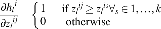
Eq. (2.48) shows that the value of the gradient is 1 for the neuron’s output with the maximum activation and 0 otherwise. The value of gradients is either 0 or 1 during SGD training, so the vanishing gradient problem is resolved easily with maxout neurons. Therefore the deep maxout neural networks are easily optimized as compared to conventional sigmoid neural networks.
2.4.2.3 Rectified Linear Units
Hinton et al. [63] proposed a new way to regularize DNNs by the use of ReLU and dropouts. Regularization is a method to reduce the overfitting in NN by preventing complex coadaptations on the training data. During training, it keeps a neuron active with some probability p, or setting it to zero otherwise. Dahl et al. [74] have shown in their research that a 5% relative reduction has been achieved in WER for cross-entropy trained DNNs using ReLU + dropout on a 50-hour English Broadcast News LVCSR. ReLU is a nonsaturated linear activation function which output zero for negative values and input itself otherwise. Its output is zero for negative values and input itself otherwise. ReLU function is defined as
Hessian-free (HF) sequence training works on two key ideas. Initially, error function is calculated by a second-order quadratic at each step then, conjugate Gradient is used to optimize the objective function. It improves the results, but is hard to implement. However, subsequent HF sequence training [75] without dropout erased some of these gains, and performance was the same as provided by a DNN trained with a sigmoid nonlinearity without dropout.
2.4.2.4 Parameterized Rectified Linear Units
ReLU units generate zero gradients whenever the units are not active. Therefore gradient-based optimization will not update their weights. The result of constant zero gradients is a slow down in the training process. To overcome this issue, He et al. [76] proposed parameterized ReLUs (PReLUs) as an advanced version of ReLU. It includes the downside to quicken the learning. It successfully obviates the vanishing gradient problem. In this model, if the input is negative then the output is produced by multiplying input with a constant variable α otherwise the output is the input itself. A PReLU function is defined as follows:
2.4.2.5 Dropout
Maxout neurons expertly manage the problem of under-fitting, so they have better optimization performance [77]. However, CNNs using maxout nonlinearity are more prone to overfitting due to their high capability. To address the overfitting problem, regularization methods such as Lp-norm, weight decay, weight tying etc. have been proposed. Hinton et al. [63] proposed a promising regularization technique called “dropout” to efficiently reduce the problem of overfitting. In this method, half of the activations within a layer are stochastically set to zero for each training sample. By doing so, the hidden units cannot coadapt to each other and learn better representation for the inputs. Model averaging is a straightforward generalization method to control the overfitting [78]. Goodfellow et al. [79] showed that dropout is an effective way to control the overfitting for maxout networks because of its better model averaging. Various strategies are used for dropout regularization for the training and testing phase. Specifically, dropout ignores each hidden unit stochastically with probability p during the feed-forward operation in neural network training.
2.5 CNN-Based End-to-End Approach
A novel acoustic model based on CNN is proposed by Palaz et al. [15], which is shown in Fig. 2.8. The CNN-based raw speech phoneme recognition system is composed of three stages. The feature learning stage modeling stage jointly perform the feature extraction and classification task. The third stage is when an HMM-based decoder is applied to learn the transition between the different classes. Initially, the raw speech signal is split into features stc = {st − c, …, st, …, st + c} in the context of 2c frames with nonoverlapped sliding window win milliseconds. The first convolutional layer learns the useful features from the raw speech signal and remaining convolutional layers further process these features into useful information. After processing the speech signal, CNN estimates the class conditional probability, for example, P(i/stc) for each class, which is used to calculate emission scaled likelihood P(stc/i). Note: the scaled likelihoods are estimated by dividing the posterior probability by the prior probability of each class, estimated by counting on the training set. Several filter stages are present in the network before the classification stage. A filter stage is a combination of a convolutional layer, a pooling layer, and nonlinearity. The joint training of filter stage and classifier stage is performed using the back-propagation algorithm.

The end-to-end approach employs the following understanding:
- 1. Speech signals are nonstationary in nature. Therefore they are processed in a short-term manner. Traditional feature extraction methods generally use 20–40 ms sliding window size. Although, in the end-to-end approach, short-term processing of the signal is required. Thus the size of the short-term window is taken as hyperparameter, which is automatically determined during training.
- 2. Feature extraction is a filter operation because its components like Fourier transform, discrete cosine transform etc. are filtering operations. In traditional systems, filtering is applied on both frequency and time. So, this factor is also considered in building convolutional layer in the end-to-end system. Therefore, the number of filters or kernel, kernel-width, and max-pooling kernel width are taken as hyperparameters that are automatically determined during training. The system automatically checks the different values of hyperparameters to get the optimal values.
The end-to-end model estimates P(i/stc) by processing the speech signal with minimal assumptions or prior knowledge.
2.6 Experiments and Their Results
Texas Instruments, Massachusetts Institute of Technology and SRI International designed (TIMIT) corpus, a popular speech dataset that is widely used for speech research. It is composed of acoustic-phonetic labels consisting of total 6300 utterances from 630 speakers of eight major dialects of American English. There are 6300 utterances that consist of two dialect sentences (SA), 450 phonetically compact sentences (SX) and 1890 phonetically diverse sentences (SI) with the exception of SA sentences which are usually excluded from the tests. The training and test sets do not overlap. It is a well-balanced corpus w.r.t. distribution of phones and triphones. Its full training set contains 4620 utterances, but usually, SI and SX sentences are used. Therefore standard 3696 SI and SX utterances are used for training. A core test set containing 192 utterances from 24 speakers is used for testing, but it is not enough for a reliable conclusion. Hence, the complete test set containing 1344 utterances from 168 speakers is also used for testing purpose in the experiments.
In the first experiment, the filter stage has a number of hyperparameters. win represents the time span of the input speech signal. kW represents the kernel that is an integral component of the layered architecture. The kernel refers to an operator applied to the input to transform it into features. dW represents the shift of temporal window. kWmp represents the max-pooling kernel width, and dWmp represents the shift of the max-pooling kernel. The value of all hyperparameters is estimated during training based on frame-level classification accuracy on training data. The experiments are conducted for three convolutional layers. The range of hyperparameters after validation is shown in Table 2.2. The best performance for the first convolutional layer is achieved with a kernel width (kW1) of 50 samples with 310 ms of context. These are hyperparameters so their value is achieved during training. Max-pooling is used as the default pooling strategy.
Table 2.2
| Hyperparameter | Units | Range |
|---|---|---|
| Input window size (win) | ms | 100–700 |
| Kernel width of the first ConvNet layer (kW1) | Samples | 10–90 |
| Kernel width of the nth ConvNet layer (kWn) | Samples | 1–11 |
| Number of filters per kernel (doutt) | Filters | 20–100 |
| Max-pooling kernel width (kWmp) | Frames | 2–6 |
| Number of hidden units in the classifier | Units | 200–1500 |
Various pooling strategies that have been successfully applied in computer vision tasks are investigated for speech recognition tasks. A local region of convolutional layer feed the input to the pooling layer that downweigh the input to generate a single output from that region. In the second experiment, pooling methods are explored for a CNN-based raw speech recognition model. To check their superiority, all the pooling strategies are evaluated on TIMIT corpus. For rest of the experiments, we used the best performing values for parameters, that is, 150 ms of context, 10, 5, and 9 frames kernel width, 10, 1, and 1 frames-shift, 100 filters and 500 hidden units. The results are shown in Table 2.3. The results show that max pooling performs well. However, these gains are not significant for speech recognition tasks as compared to gains achieved in vision tasks [80]. The results are approximately the same, that is, minor difference in recognition rate for all pooling strategies for training and testing set. In the results, MOP and spectral pooling shows a performance drop. The phone error rate (PER) offered by pooling strategies like Lp pooling and stochastic pooling is high as compared to max pooling. Note that MOP and spectral pooling also degrade the performance of ASR systems. The experiments conclude that different pooling strategies are not showing any drastic improvement for speech recognition than it is for other domains such as image classification [81].
Table 2.3
| Pooling Strategy | PER (%) | |
|---|---|---|
| Training Set | Testing | |
| Max pooling | 19.4 | 21.9 |
| Average pooling | 19.9 | 22.1 |
| Stochastic pooling | 20.0 | 22.1 |
| Lp pooling | 19.7 | 22.0 |
| Mixed pooling | 19.7 | 22.0 |
| Multiscale orderless pooling | 20.1 | 22.3 |
| Spectral pooling | 20.0 | 22.2 |

In the third experiment, the parameters are the same as the ones used in the second experiment. The performance of different nonlinear functions, for example, sigmoid, maxout, ReLU, and PReLU is evaluated by performing the experiments on fully connected layers with and without using dropout networks on the TIMIT dataset. The experimental results of different nonlinear networks with or without dropout are shown in Table 2.4. Maxout networks converge faster than ReLU, PReLU, and sigmoidal networks. The PER is the same for sigmoid in both cases with or without dropout. During training, the maxout networks show better abilities to fit the training dataset. During testing, the maxout and the PReLU networks have shown almost the same PER, but the sigmoidal and ReLU perform less. Further, the model is evaluated for dropout. The same dropout rate is applied for each layer. Dropout is varied with the step size 0.05. The experiments confirmed that the dropout probability p = 0.5 is reasonable.
Table 2.4
| Nonlinearity | Model | PER (%) | |
|---|---|---|---|
| Training Set | Testing Set | ||
| Sigmoid | No-Drop | 21.1 | 22.9 |
| Sigmoid | Dropout | 21.0 | 22.9 |
| Maxout | No-Drop | 20.6 | 22.5 |
| Maxout | Dropout | 19.9 | 21.9 |
| ReLU | No-Drop | 21.2 | 23.0 |
| ReLU | Dropout | 20.1 | 22.2 |
| PReLU | No-Drop | 20.6 | 22.6 |
| PReLU | Dropout | 20.0 | 22.1 |

Table 2.5 shows the comparison of existing end-to-end speech recognition model in the context of PER. The evaluated model is not the best model, but it is satisfactory. The result of the experiment conducted on the TIMIT dataset for this model is compared with already existing techniques, and they are shown in Table 2.6. The main advantages of this model is that it offers close performance by directly using the raw speech. It also increases the generalization capability of the classifiers.
Table 2.5
| End-to-End Speech Recognition Model | PER (%) |
|---|---|
| CNN-based speech recognition system using raw speech as input [17] | 33.2 |
| Estimating phoneme class conditional probabilities from raw speech signal using CNNs [41] | 32.4 |
| CNNs-based continuous speech recognition using raw speech signal [16] | 32.3 |
| End-to-end phoneme sequence recognition using CNNs [15] | 27.2 |
| CNN-based direct raw speech model | 21.9 |
| End-to-end continuous speech recognition using attention-based recurrent NN: first results [28] | 18.57 |
| Towards end-to-end speech recognition with deep CNNs [49] | 18.2 |
| Attention-based models for speech recognition [7] | 17.6 |
| Segmental RNNs for end-to-end speech recognition [82] | 17.3 |
Table 2.6
| Methods | PER (%) |
|---|---|
| GMM/HMM-based ASR system [83] | 34 |
| CNN-based direct raw speech model | 21.9 |
| Attention-based models for speech recognition [7] | 17.6 |
| Segmental RNNs for end-to-end speech recognition [82] | 17.3 |
| Combining time and frequency domain convolution in CNN-based phone recognition [52] | 16.7 |
| Phone recognition with hierarchical convolutional deep maxout networks [84] | 16.5 |
2.7 Conclusion
The CNN-based direct raw speech recognition model directly learns the relevant representation from the speech signal in a data-driven method and calculates the conditional probability for each phoneme class. In this, CNN as an acoustic model, consists of a feature stage and classifier stage. Both the stages are trained jointly. Raw speech is supplied as input to the first convolutional layer, and several convolutional layers further process it. Classifiers like ANN, CRF, MLP or fully connected layers, calculate the conditional probabilities for each phoneme class. Afterwards, decoding is performed using HMM. This model shows the better performance as shown by MFCC-based conventional model.