
Exchange Rates, Interest Rates, and Interest Parity
Abstract
In this chapter, the relationship between interest rates and exchange rates are examined, and consideration is given to how exchange rates adjust to achieve equilibrium in financial markets. An example is worked through showing how covered interest arbitrage works, with a discussion of how well interest rate parity holds in the real world, with several reasons given for the deviations in interest rate parity that do occur. The differences between nominal and real interest rates are described, along with the role of inflation in determining interest rates. The Fisher equation and the interest parity equation are discussed as a means to determine how interest rates, inflation, and exchange rates are all linked. The term structure of interest rates is defined as the structure of interest rates existing on investment opportunities over time; the several competing theories that explain this are discussed in detail, with real-world examples.
Keywords
Approximate covered interest rate parity; covered interest rate arbitrage; effective return on investment; exact interest rate parity; exchange rate; expected exchange rate; Fisher effect; Fisher equation; interest rate parity; nominal interest rate; real interest rate; term structure of interest rates
International trade occurs in both goods and financial assets. Exchange rates change in a manner to accommodate this trade. In this chapter, we study the relationship between interest rates and exchange rates, and consider how exchange rates adjust to achieve equilibrium in financial markets.
Interest Rate Parity
The interest rate parity explains the relationship between returns to bond investments between two countries. Interest rate parity results from profit-seeking arbitrage activity, specifically covered interest rate arbitrage. Let us go through an example of how covered interest arbitrage works. For expositional purposes
i$=interest rate in the United States
i£=interest rate in the United Kingdom
where the interest rates and the forward rate are for assets with the same term to maturity (e.g., 3 months or 1 year), the investor in the United States can earn (1+i$) at home by investing $1 for 1 period (for instance, 1 year). Alternatively the US investor can invest in the United Kingdom by converting dollars to pounds and then investing the pounds. Here $1 is equal to 1/E pounds (where E is the dollar price of pounds). Thus by investing in the United Kingdom, the US resident can earn (1+i£)/E. This is the quantity of pounds resulting from the $1 invested. Remember $1 buys 1/E pounds, and £1 will return 1+i£ after 1 period. Thus 1/E pounds will return (1+i£)/E after 1 period.
Since the investor is a resident of the United States, the investment return will ultimately be converted into dollars. But since future spot exchange rates are not known with certainty, the investor can eliminate the uncertainty regarding the future dollar value of (1 +i£)/E by covering the £ currency investment with a forward contract. By selling (1+i£)/E pounds to be received in a future period in the forward market today, the investor has guaranteed a certain dollar value of the pound investment opportunity. The covered return is equal to (1+i£)F/E dollars. The US investor can earn either 1+i$ dollars by investing $1 at home or (1+i£)F/E dollars by investing the dollar in the United Kingdom. Arbitrage between the two investment opportunities results in
which can be rewritten as:
(6.1)
Eq. (6.1) can be put in a more useful form by subtracting 1 from both sides, giving us the exact interest rate parity equation:
(6.2)
This equation can be approximated by noting that the denominator on the left side is almost one. Approximating by assuming that the denominator is equal to one results in the approximate covered interest rate parity equation:
(6.3)
The smaller i£, the better the approximation of Eqs. (6.3) to (6.2). Eq. (6.3) indicates that the interest differential between a comparable US and UK investment is equal to the forward premium or discount on the pound. (We must remember that, since interest rates are quoted at annual rates or percent per annum, the forward premiums or discounts must also be quoted at annual rates.) Now let us consider an example. Ignoring bid-ask spreads, we observe the following Eurocurrency market interest rates:
The exchange rate is quoted as the dollar price of pounds and is currently E=2.00. Given the previous information, what do you expect the 12-month forward rate to be?
Using Eq. (6.3) we can plug in the known values for the interest rates and spot exchange rate and then solve for the forward rate:
which simplifies to
Thus we would expect a 12-month forward rate of $2.10 to give a 12-month forward premium equal to the 0.05 interest differential.
Suppose a bank sets the 12-month forward rate at $2.15, instead of $2.10. This would lead to arbitrage opportunities. How would the arbitragers profit? They could buy pounds at the spot rate and then invest and sell the pounds forward for dollars, because the future price of pounds is higher than that implied by the interest parity relation. These actions would tend to increase the spot rate and lower the forward rate, thereby bringing the forward premium back in line with the interest differential. The interest rates could also move, because the movement of funds into pound investments would tend to depress the pound interest rate, whereas the shift out of dollar investments would tend to raise the dollar rate.
Effective Return on a Foreign Investment
The interest parity relationship can also be used to illustrate the concept of the effective return on a foreign investment. Eq. (6.3) can be rewritten so that the dollar interest rate is equal to the pound rate plus the forward premium. Thus the returns to investing in dollar assets and pound denominated assets are:
(6.4)
Covered interest parity ensures that Eq. (6.4) will hold. Note that the interest rate on the bond i£ is not the relevant return measure by itself, since this is the return in pounds. Instead the effective return to a UK investment is composed of an interest rate return and an exchange rate return. But suppose we do not use the forward market, yet we are US residents who buy UK bonds. Even in this case the effective return would be composed of two parts. The first part would be the interest rate return and the second would be the expected change in the exchange rate, as we now need to take into account the expected spot rate in the future. In other words, the return on a UK investment, plus the expected change in the value of UK currency, is our expected return on a pound investment. If the forward exchange rate is equal to the expected future spot rate, then the forward premium is also the expected change in the exchange rate.
Deviations From Covered Interest Rate Parity
Even though foreign exchange traders quote forward rates based on interest differentials and current spot rates so that the forward rate will yield a forward premium equal to the interest differential, we may ask: How well does interest rate parity hold in the real world? Since deviations from interest rate parity would seem to present profitable arbitrage opportunities, we would expect profit-seeking arbitragers to eliminate any deviations. Still, careful studies of the data indicate that small deviations from interest rate parity do occur. There are several reasons why interest rate parity may not hold exactly, and yet we can earn no arbitrage profits from the situation. The most obvious reason is the transactions cost between markets. Because buying and selling foreign exchange and international securities involves a cost for each transaction, there may exist deviations from interest rate parity that are equal to, or smaller than, these transaction costs. In this case, speculators cannot profit from the deviations, since the price of buying and selling in the market would wipe out any apparent gain. Studies indicate that for comparable financial assets that differ only in terms of currency of denomination (e.g., dollar- and pound-denominated Eurodeposits in a German bank), 100% of the deviations from interest rate parity can be accounted for by transaction costs.
Besides transaction costs, there are other reasons why interest rate parity may not hold perfectly. One other reason, for small deviations from interest rate parity, is the potential difference in taxation of interest earnings and foreign exchange rate earnings. If these are differently taxed in a country then the effective return Eq. (6.4) might not hold since one side involves only interest earnings and the other interest earnings and foreign exchange earnings. Thus it may be misleading to simply consider pretax effective returns to decide if profitable arbitrage is possible.
Two more reasons for why interest rate parity might not hold perfectly are government controls and political risk. If government controls on financial capital flows exist, then an effective barrier between national markets is in place. If an individual cannot freely buy or sell the currency or securities of a country, then the free market forces that work in response to effective return differentials will not function. Indeed, even the threat of controls could affect the interest rate parity condition. Political risk is often mentioned in conjunction with government controls. The interest rate parity condition is not directly affected by political risk, such as a regime change. Instead it is the threat of the new regime imposing capital controls that affects the interest rate parity condition. We should note, however, that the external or Eurocurrency market often serves as a means of avoiding political risk, since an individual can borrow and lend foreign currencies outside the home country of each currency. For instance, the Eurodollar market provides a market for US dollar loans and deposits in major financial centers outside the United States, thereby avoiding any risk associated with US government actions.
Interest Rates and Inflation
To better understand the relationship between interest rates and exchange rates, we now consider how inflation can be related to both. To link exchange rates, interest rates, and inflation, we must first understand the role of inflation in interest rate determination. Economists distinguish between real and nominal rates of interest. The nominal interest rate is the rate actually observed in the market. The real rate is a concept that measures the return after adjusting for inflation. If you lend someone money and charge that person 5% interest on the loan, the real return on your loan is less when there is inflation. For instance, if the rate of inflation is 10%, then the debtor will pay back the loan with dollars that are worth less. In fact, so much less that you, the lender, end up with less purchasing power than you had when you initially made the loan.
This all means that the nominal rate of interest will tend to incorporate inflation expectations in order to provide lenders with a real return for the use of their money. The expected effect of inflation on the nominal interest rate is often called the Fisher effect (after Irving Fisher, a pioneer of the determinants of interest rates), and the relationship between inflation and interest rates is given by the Fisher equation:
(6.5)
where i is the nominal interest rate, r the real rate, and πe the expected rate of inflation. Thus an increase in πe will tend to increase i. For example, the fact that interest rates in the 1970s were much higher than in the 1960s is the result of higher inflationary expectations in the 1970s. Across countries, at a specific time, we should expect interest rates to vary with inflation. Table 6.1 shows that nominal interest rates tend to be higher in countries that have recently experienced higher rates of inflation.
Table 6.1
Interest rates and inflation rates for selected countries
| Country | Inflation rate (%) | Interest rate (%) |
| Portugal | −0.20 | 0.95 |
| South Korea | 1.30 | 2.00 |
| United States | 1.60 | 1.25 |
| Turkey | 8.90 | 10.75 |
| Argentina | 36.40 | 26.15 |
Source: CIA World Factbook, 2014; www.deposits.org, Sep. 2015.
Exchange Rates, Interest Rates, and Inflation
If we combine the Fisher Eq. (6.5) and the interest parity Eq. (6.3), we can determine how interest rates, inflation, and exchange rates are all linked. First, consider the Fisher equation for the United States and the United Kingdom:
and
Global investors now want to have as high as possible real returns from their investments. If global markets allow free flow of capital, one might expect that the real returns across countries equalize. If we assume that the real rate of interest is the same internationally, then r$=r£. In this case, the nominal interest rates, i$ and i£, differ solely by expected inflation, so we can write
(6.6)
The interest parity condition of Eq. (6.3) indicates that the interest differential is also equal to the forward premium, or
(6.7)
Eq. (6.7) summarizes the link among interest, inflation, and exchange rates.
In the real world the interrelationships summarized by Eq. (6.7) are determined simultaneously, because interest rates, inflation expectations, and exchange rates are jointly affected by new events and information. For instance, suppose we begin from a situation of equilibrium, where interest parity holds. Suddenly there is a change in US policy that leads to expectations of a higher US inflation rate. The increase in expected inflation will cause dollar interest rates to rise. At the same time exchange rates will adjust to maintain interest parity. If the expected future spot rate is changed, we would expect F to carry much of the adjustment burden. If the expected future spot rate is unchanged, the current spot rate would tend to carry the bulk of the adjustment burden. Finally if central bank intervention is pegging exchange rates at fixed levels by buying and selling to maintain the fixed rate, the domestic and foreign currency interest rates will have to adjust to parity levels. The fundamental point is that the initial US policy change led to changes in inflationary expectations, interest rates, and exchange rates simultaneously, since they all adjust to new equilibrium levels.
Expected Exchange Rates and the Term Structure of Interest Rates
There is no such thing as the interest rate for a country. Interest rates within a country vary for different investment opportunities and for different maturity dates on similar investment opportunities. The structure of interest rates existing on investment opportunities over time is known as the term structure of interest rates. For instance in the bond market we will observe 3-month, 6-month, 1-year, 3-year, and even longer-term bonds. If the interest rates rise with the term to maturity, then we observe a rising term structure. If the interest rates are the same regardless of term, then the term structure will be flat. We describe the term structure of interest rates by describing the slope of a line connecting the various points in time at which we observe interest rates.
There are several competing theories that explain the term structure of interest rates. We will discuss three theories:
1. Expectations: This theory suggests that the long-term interest rate tends to be equal to an average of short-term rates expected over the long-term holding period. In other words an investor could buy a long-term bond or a series of short-term bonds, so the expected return from the long-term bond will tend to be equal to the return generated from holding the series of short-term bonds.
2. Liquidity premium: Underlying this theory is the idea that long-term bonds incorporate a risk premium since risk-averse investors would prefer to lend short term. The premium on long-term bonds would tend to result in interest rates rising with the holding period of the bond.
3. Preferred habitat: This approach contends that the bond markets are segmented by maturities. In other words there is a separate market for short- and long-term bonds, and the interest rates are determined by supply and demand in each market. If the markets are segmented then the returns in the long-term bond market can be very different from the short-term bond market.
Although we could use these theories to explain the term structure of interest rates in any one currency, in international finance we use the term structures for different currencies to infer expected exchange rate changes. For instance if we compared Euro–dollar and Euro–euro deposit rates for different maturities, like 1-month and 3-month deposits, the difference between the two term structures should reflect expected exchange rate changes, as long as the expected future spot rate is equal to the forward rate. Of course, if there are capital controls, then the various national markets become isolated and there would not be any particular relationship between international interest rates.
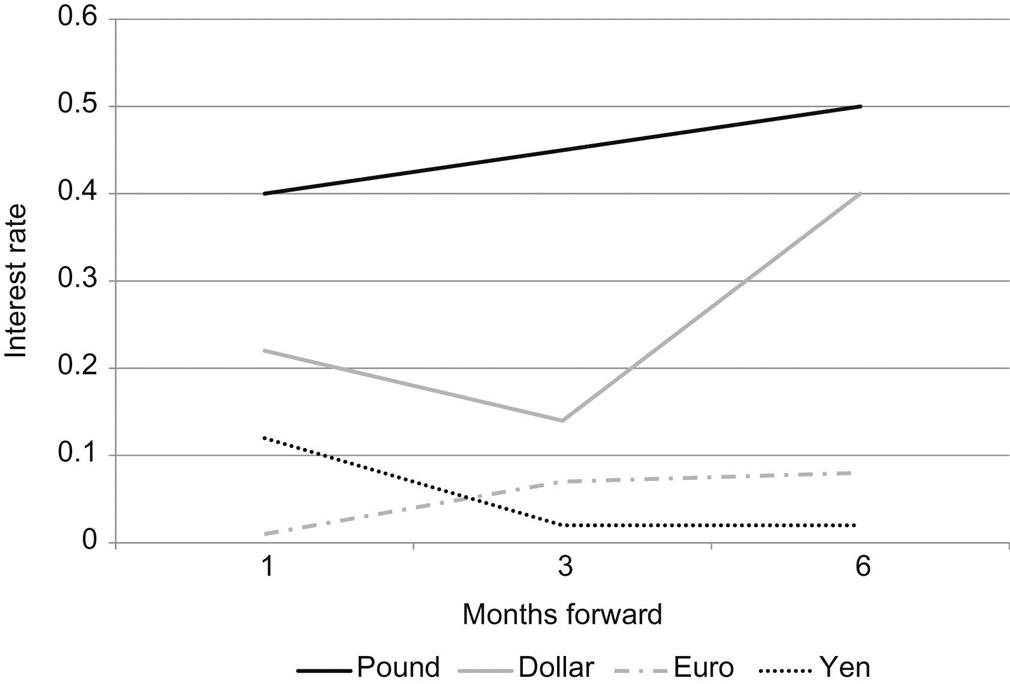
Fig. 6.1 plots the Eurocurrency deposit rates at a particular time for 1- to 6-month terms. We know from the interest rate parity condition that when one country has higher interest rates than another, the high-interest-rate currency is expected to depreciate relative to the low-interest-rate currency. The only way an interest rate can be above another one is if the high-interest-rate currency is expected to depreciate; thus, the effective rate, i+(F−E)/E (as shown in Eq. (6.4), with the forward rate used as a predictor of the future spot rate), is lower than the observed rate, i, because of the expected depreciation of the currency (F<E).
If the distance between two of the term structure lines is the same at each point, then the expected change in the exchange rate will be constant. To see this more clearly, let us once again consider the interest parity relation given by Eq. (6.3):
This expression indicates that the difference between the interest rate in two countries will be equal to the forward premium or discount when the interest rates and the forward rate reflect the same term to maturity. If the forward rate is equal to the future spot rate, then we can say that the interest differential is also approximately equal to the expected change in the spot rate. This means that at each point in the term structure, the difference between the national interest rates should reflect the expected change in the exchange rate for the two currencies being compared. By examining the different points in the term structure, we can determine how the exchange rate expectations are changing through time. One implication of this is that even if we did not have a forward exchange market in a currency, the interest differential between that currency and other currencies would allow us to infer expected future exchange rates.
Now we can understand why a constant differential between two interest rates implies that future changes in the exchange rate are expected to occur at some constant rate. Thus if two of the term structure lines are parallel, then the exchange rate changes are expected to be constant (the currencies will appreciate or depreciate against each other at a constant rate). On the other hand, if two term structure lines are diverging, or moving farther apart from one another, then the high-interest-rate currency is expected to depreciate at an increasing rate over time. For term structure lines that are converging, or moving closer together, the high-interest-rate currency is expected to depreciate at a declining rate relative to the low-interest-rate currency.
To illustrate the exchange rate–term structure relationship, let us look at Fig. 6.1. In Fig. 6.1 the term structure line for the yen lies below that of the dollar. We should then expect the Japanese yen to appreciate against the US dollar and the yen should sell at a forward premium against the dollar. With regard to the slopes of the curves, the term structure line for Japan and the United States are diverging over time. The divergence of the US line from the Japanese line suggests that the yen is expected to appreciate against the dollar at a faster rate over time.
Looking at the other currencies in Fig. 6.1 we can see differences in the expected changes in the exchange rates. The term structure line for the pound lies above that of the dollar so we should expect the pound to depreciate in value against the dollar and sell at a forward discount against the dollar. The fact that the term structure of the euro lies below both the pound and dollar indicates that the euro is expected to appreciate against both of those currencies in the table. A particularly interesting case is the term structure for the euro and the yen, because these intersect. The yen is expected to depreciate or sell at a forward discount against the euro at 1-month maturity, but at the 3-month and 6-month maturities the yen sells at forward premium against the euro.
Summary
1. The interest parity relationship indicates that the interest rate differential between investments in two currencies will equal to the forward premium or discount between the currencies.
2. The international investment is covered when investors use the forward contracts to cover or hedge themselves from risk of the unknown future spot exchange rates.
3. A currency is at a forward premium (discount) by as much as its interest rate is lower (higher) than the interest rate in the other country.
4. Covered interest parity links together four rates, which are the current spot exchange rate, the current forward exchange rate, and the current interest rates in two countries. If one of these rates change, at least one of the others must also change to maintain the covered interest parity.
5. Covered interest arbitrage ensures interest parity.
6. Deviations from interest rate parity could be the result of transaction costs, differential taxation, government controls, or political risk.
7. The real interest rate is equal to the nominal interest rate minus the expected rate of inflation.
8. If real interest rates are equal in two countries, then the interest rate differential will equal to expected inflation rate differential, which in turn will equal to the forward premium or discount between two currencies.
9. The term structure of interest rates is the relationship between interest rates on various bonds with different terms to maturity.
10. Differences between the term structure of interest rates in two countries will reflect the expected exchange rate changes.
Exercises
1. Suppose you want to infer expected future exchange rates in a less developed country that has free-market-determined interest rates but does not have a forward exchange market. Is there any other way of inferring expected future exchange rates? Under what assumptions?
a. Show that there is a direct relationship between the forward premium and the “real” interest rate differential between two currencies.
b. Under what conditions will the forward premium equal the expected “inflation” differential between two currencies?
3. Give four reasons why, when interest parity does not hold exactly, we are unable to take advantage of arbitrage to earn profits.
4. Suppose the 1-year interest rate on British pounds is 11%, the dollar interest rate is 6%, and the current $/£ spot rate is $1.80.
a. What do you expect the spot rate to be in 1 year?
b. Why can we not observe the expected future spot rate?
5. Assume that the 1-year interest rate in the United States is 2% and the 1-year interest rate in Sweden is 4%. Is there a premium or discount on the Swedish krona?
6. If two countries had identical term structures of interest rates, what is the expected future exchange rate change between the two currencies?
Appendix A What are Logarithms, and Why are They Used in Financial Research?
Although this is not a course in mathematics, there are certain techniques that are so prevalent in modern financial research that not to use them would be a disservice to the student. Logarithms are a prime example. The most important reason for the use of logarithms is that they show the “true” percentage distance. In addition, they facilitate calculations in financial relationships.
What are Logarithms?
Logarithms are a way of transforming numbers to simplify mathematical analysis of a problem. One way to view a logarithm as the power to which some base must be raised to give a certain number. For example, we all know that the square of 10 is 100, or 102=100. Therefore if 10 is our base, we know that 10 must be raised to the second power to equal 100. We could then say that the logarithm of 100 to the base 10 is 2. This is written as
What then is the log10 of 1000? Of course, log10 1000=3, because
In general any number greater than 1 could serve as the base by which we could write all positive numbers. Picking any arbitrary number designated as a, where a is greater than 1, we could write any positive number b as
where c is the power to which a must be raised to equal b.
Rather than pick any arbitrary number for our base a, there is a particular number that arises naturally in economic phenomena. This number is approximately 2.71828, and it is called e. The value of e arises in the continuous compounding of interest. Specifically, e=limn→∞(1+1/n)n, where n is the number of times interest is compounded per year. The value of some principal amount, P, in 1 year, compounded continuously at r percent interest, is V=Per. If r=100%, then the amount of principal and interest after 1 year is V=Pe. Since e comes naturally out of continuous compounding, we refer to e as the base of the natural logarithms. Financial researchers utilize logarithms to the base e. Rather than write the log of some number b as logeb=c, it is common to express loge as ln, so that we write
In all uses of logarithms in this text, we assume log b is actually ln b or the natural logarithm; it is for convenience that we drop the e subscript and simply write log b rather than logeb.
Why Use Logarithms in Financial Research?
If the lesson so far has seemed rather esoteric and unrelated to your interests, here is the payoff.
A useful feature of logarithms is that the change in the logarithm of some variable is commonly used to measure the percentage change in the variable (the measure is precise for compound changes and approximate for simple rates of change). If we want to calculate the percentage change in the yen/$ exchange rate (E) between today (period t) and yesterday (period t−1), we could calculate (Et−Et−1)/Et−1. Alternatively we could calculate ln Et−ln Et−1.
For example, let us assume that the Et−1=80 for the yen/$ in the past value and Et=125 for the yen/$ in the current period. What is the percentage change in the value of the yen? If we use the formula (Et−Et−1)/Et−1 then the percentage change is 56.25%, but if we use the ln Et−ln Et−1=44.63%. The two values are near each other, but not quite the same. Now assume that the exchange rate was quoted in inverse form instead as $/yen. The rates become Et−1=0.0125 for the yen/$ and Et=0.008. Note that these are identical to the rates quoted above. What is the percentage change in the value of the yen? If we use the formula (Et−Et−1)/Et−1 then the percentage change is −36%, but if we use the ln Et−ln Et−1=−44.63%. So when we use natural logarithms the percentage distance becomes identical no matter how currencies are quoted.
The fact that percentage distances are the same, whatever the base period value, is a very convenient feature of logarithms. In the Covered Interest Rate Parity concept, we need to be able to move back and forth in currencies, and using natural logarithms we know that this will equal the interest rate differentials.
Natural logarithms also have some convenient mathematical properties. Three extremely helpful properties of logarithms that are used frequently in international finance are:
1. The log of a product of two numbers is equal to the sum of the logs of the individual numbers:
2. The log of a quotient is equal to the difference of the logs of the individual numbers:
3. The log of some number M raised to the N power is equal to N times the log of M:
Since many relationships in financial research are products or ratios, by taking the logs of these relationships, we are able to analyze simple, linear, additive relationships rather than more complex phenomena involving products and quotients.
This appendix serves as a brief introduction or review of logarithms. Rather than provide more illustrations of the specific use of logarithms in international finance, at this point it is preferable to study the examples that arise in the context of the problems, as analyzed in subsequent chapters. More general examples of the use of logarithms may be found in Wainwright and Chiang (2004).