Chapter 4. Using Power BI Desktop

In Chapter 3, we introduced the concept of data refresh. Contoso’s manager of budgeting, David, was able to refresh a Power BI model, based on a Microsoft Excel workbook that contains sales for the last three years and forecasts for the next year. To perform that, he had to learn the basics of Power BI Desktop, a Windows application that brings the full modeling power of Power BI to your desktop.

In this chapter, David will move a few steps further in building his Power BI model. But, the solution he has built so far still depends on IT providing him with the sales figures for the last three years. Fortunately, David discovers that Power BI Desktop can load the numbers directly from the Contoso data warehouse via Microsoft SQL Server. Now, when Power BI carries out data refresh, it will automatically get the latest sales data, updating the entire model.

Let’s take a brief look at what David needs to do:

• Load sales figures from the data warehouse instead of using his Excel file. This requires accessing the corporate database, but the IT department can give him access to the data he needs.

• Load forecasts for the next year from the Excel file that the country/region managers update every day.

Power BI Desktop offers all of the functionalities that David requires. Now, let’s go deeper and learn how to take advantage of this extremely useful application.

Karin is happy to do so because she will no longer need to fill the Excel workbook. If David can load the data and manage to grab insights by himself, her daily list of chores will become lighter. Thus, Karin tells David, “You can access the view named Sales2015 using your Windows credentials on the server ContosoDbServer.” David’s account can only read that view, so there is no potential danger. Database security will guarantee that nothing bad can happen to the database.

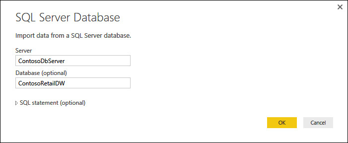
In Power BI Desktop, on the Home tab, David uses the Get Data function, this time using the SQL Server option. In the dialog box that opens, he provides the connection information Karin gave him (see Figure 4-1) and then clicks OK.

Power BI Desktop connects to the database and presents a list of data tables, which includes the one that Karin created, Sales2015. When David clicks it, Power BI Desktop shows a preview of the content, as depicted in Figure 4-2.

After David makes his selection and clicks Load. Power BI Desktop asks how he wants to interact with the data. He selects Import and then clicks OK, as illustrated in Figure 4-3.

Let’s take a moment to learn about this connection option because it is an important one and will help shed more light on how Power BI connections work.

When you choose Import, Power BI Desktop connects to the database, loads the information, and stores it within its internal data model. You can then work on your data in Power BI Desktop without being connected to the database. You will only need a connection when you want to refresh the data.

With DirectQuery, Power BI Desktop does not load the data into its internal database. Instead, it runs a query to the original database every time it needs to draw a chart or, in general, run a query. Thus, the connection between Power BI Desktop and the database will be permanent.

The contrast in the query timings reflects a key difference: when you use Import, you are working with data that is only as current as the latest refresh, whereas with DirectQuery you always see the latest information available when you create the report.

At first glance, it looks like DirectQuery is the most convenient method for loading data, but this is not totally true. If the data is updated frequently, it is very likely that one minute you will see a report with a set of figures, but when you open it again a few minutes later, the numbers might no longer be the same. This is frustrating if you are analyzing information over the span of an entire year (which is what David is doing). Numbers that change too frequently can become disturbing. Also, although real-time data might sometimes be useful, it comes at the cost of query speed; DirectQuery by its very nature is much slower than working with data that is resident on your device and directly accessible by Power BI Desktop.

As a final note, keep in mind that DirectQuery works fine when you use Power BI Desktop on your laptop, but when you publish the model to Power BI, the cloud service needs a way to communicate with the internal database server. This is accomplished by using the Enterprise Gateway, which is the advanced version of the Personal Gateway, to which you were introduced in Chapter 3.

As mentioned just a moment ago, David wants to analyze data over the span of a year, so he does not need his figure to be updated constantly; thus, he chooses Import and, after a few seconds, the loading process finishes. He notices that the name of the table is too long. In fact, Power BI Desktop used the full name of the table (including the schema name), but you can easily give it a new name by right-clicking it and then, on the shortcut menu that opens, select Rename, as demonstrated in Figure 4-4.

After he renames the table, there seems to be no difference between this model and the previous ones that he created by loading data from Excel. In reality, there is a big difference: now, the Power BI model is linked to the original source of data, which is the SQL Server database. When Power BI Desktop refreshes the information, it does not need the Excel file (which if you recall was manually updated by David and Karin). Instead, by connecting directly to the database, it always gathers the latest information available at the moment of refresh. In other words, David eliminated Excel as a middle step, saving the time and effort required to prepare that file.

To solve this problem, we need to dive a bit more into the internal structure of the Power BI Desktop model. In Chapter 3, we said that a Power BI Desktop model contains an internal query, created by Power BI Desktop, for each dataset. This internal query is not visible if you perform basic operations, such as loading data from an Excel file or from a SQL Server database. Yet, it is there, and if you need to modify it, you can.

The query language of Power BI Desktop is used by Query Editor, and discussion of that language alone would fill an entire book of several hundred pages. As you might imagine, we cannot cover it in a mere few pages here. Instead, we want to show you some basic features of Query Editor so that you better understand its capabilities.

To modify a Query Editor script, on the Power BI Desktop ribbon, on the Home tab, click Edit Queries, as shown in Figure 4-5.

Query Editor opens in a new window, presenting myriad options, as depicted in Figure 4-6.

Let’s take a quick tour of the Query Editor window. Along the top is the ribbon, which has four tabs: Home, Transform, Add Column, and View. Below the ribbon, on the left side, is the Query pane, which displays a list of all the queries for the model. The middle pane shows the result of the query. The Query Settings pane on the right displays the query properties.

In David’s scenario, he is already accessing the 2015 sales data from the Contoso database, so the objective now is to create a new query that also retrieves the budget forecast information from the Excel workbook.

To load data from a new dataset, on the ribbon, in the New Query group of the Home tab, click New Source, and then specify to load the data from the Budget table. (The process is nearly identical to what you already learned in Chapter 3.) This results in two tables in the Queries pane on the left side of the Query Editor window, as demonstrated in Figure 4-7.

When you are finished editing, on the ribbon, on the Home tab, click Close & Apply to load the data into Power BI Desktop. When this is done, the Power BI Desktop Fields pane shows the two sources: the table in Excel, and the SQL Server table in the Contoso database, as depicted in Figure 4-8.

The chart is confusing, at the very least. David used the Brand and Sales2015 attributes from the Sales2015 table, and the Budget 2016 column from the Budget table. Nevertheless, the values shown for the budget are always the same. Moreover, the value looks to be too high for each brand.

The problem here is that if you use the Brand column from the Sales2015 table, despite having the same name, it is not the same as using the Brand column from the Budget table. The two columns have the same values and the same name, but they are not the same column. In fact, if you were to try replacing Brand in the chart with the Brand column from the Budget table, the result would be similar, but with the opposite behavior. Figure 4-10 shows that by using the Brand column from the Budget table, the budget values are now correctly sliced, but the sales are not.

This would be a good time to digress and discuss what the correct data model to represent David’s dataset is. It would be useful, but somewhat pedantic and not very relevant to the objectives of this book. The important point here is that you cannot slice numbers coming from two tables using columns from only one of them, unless the two tables share some kind of relationship.

To solve the problem, you need to bring the Budget 2016 column from the Excel Budget table into the Sales2015 table, exactly where it was in the original Excel file. Using the technical terms, we say that you need to join the two tables together, copying the Budget column for the given country/region and brand. It turns out that Power BI Desktop’s Query Editor is the perfect tool to perform such an operation.

In fact, with Query Editor you can load tables in an easy way, but, as we said earlier, you also have the option of editing the autogenerated query to make it behave differently. Let’s catch up with David to see how he does this.

David goes back to the Power BI Desktop Query Editor window and modifies the Sales 2015 query. He selects the Sales 2015 query and then, on the ribbon, on the Home tab, he clicks Merge Queries (see Figure 4-11).

This opens the Merge dialog box, in which you need to specify the destination table (the source is the one selected) and which columns to use to join them together. In David’s case, the columns to use are CountryRegion and Brand, in both tables, as illustrated in Figure 4-12.

When you are selecting the columns to merge, Query Editor might display a dialog box similar to that shown in Figure 4-13, asking you for the privacy level of the data sources.

Privacy levels are used to ensure that you do not send private information to data sources outside of your secure area. Setting the wrong privacy level might expose sensitive data to untrusted sources or might affect the performance of the query. In David’s case, he sets both sources to Private because both sources are within its network. If you are loading data from the web, for example, you should mark that data source as Public; this will avoid sending information to the web that is coming from one private source.

The last option available in the Merge dialog box is Join Kind. You use this to choose what happens with rows in one table that have no corresponding rows in the other table. For example, if there are sales for a country/region but there is no budget for it, should that country/region be included in the resulting dataset? The most typical kind of join is the default: a Left Outer join, which includes all the rows from the source table and only matching rows from the merged one. In other words, in David’s case, it retrieves all the sales, plus the budget for the countries/regions and brands with sales.

After David clicks OK, the table shows a new column named NewColumn, whose content is from a table, as shown in Figure 4-14.

In fact, when you merge two tables, the result is the original column, plus a new column of type Table. This new column contains all of the rows that are related with the current row in the original table. In David’s case, the table contains a single row, but, for more complex joins, it might contain many rows.

David is not interested in retrieving the full table. Instead, he wants only the Budget column. To do this, he needs to expand the NewColumn table so that it includes only the columns he wants. He can do this easily by clicking the two arrows adjacent to the column name, in the yellow box around the column. This opens the expand column dialog box, as illustrated in Figure 4-15.

In the example, David selected only the Budget 2016 column. The result of this is that instead of NewColumn, you now have the Budget 2016 column for each row of the Sales table, as depicted in Figure 4-16.

David is nearly done. The last step is that the column, as it is, shows the full yearly budget, whereas the Sales table should contain only the monthly budget. In Excel, David divided the budget value by 12; hence, he is doing the same here. To perform this, on the ribbon, on the Add Column tab, he clicks Add Custom Column (in the General group) to create a new column containing the value of Budget 2016 divided by 12, as demonstrated in Figure 4-17.

To create a new column, David must provide the expression that computes it. He can do that in the Add Custom Column dialog box that opens, as shown in Figure 4-18.

Figure 4-19 presents the result of all these steps, in which you can see the newly computed Budget column.

As a final step, David right-clicks and removes the Budget 2016 column, which is no longer useful.

Before saving the query, David needs to perform a final step: he defines the data type of the column. By default, custom columns are of the Any data type, meaning that the data type is not defined. But, because he wants to use it to aggregate values (which are, numbers), he must change the data type to Decimal Number, as shown in Figure 4-20.

When this work is done, David ends up with a Sales2015 table that looks identical to that of its Excel counterpart. The big difference now is that the value of sales is computed from the SQL Server database and, when the model is refreshed, it will retrieve the latest figures in the Sales2015 table, with no manual intervention.

You can resolve the issue in either of two ways: hide the Budget table from the Fields list, or avoid loading it altogether. To hide a table, in the Fields pane, right-click the table name and then, on the shortcut menu that opens, click Hide, as depicted in Figure 4-21.

A hidden table, as its name implies, is no longer visible in the Fields pane. You can always make it visible again by choosing View Hidden from the context menu of any table of the field pane and then clearing the Hide check mark. Keep in mind that hiding a table does not mean it is at all secure. A hidden table is only marked as not visible, but any user can see it by simply using the user interface; hiding a table simply makes the model easier to browse and less error-prone.

In David’s case, he would prefer to avoid loading the table altogether. In fact, all of the information needed to build the reports is now stored in the Sales 2015 table. The Budget table is used by Query Editor to merge the budget (divided by 12) into Sales 2015. After the budget information is stored in Sales 2015, the Budget table is redundant and does not need to be loaded.

To avoid loading a table, in Query Editor, in the Queries pane, right-click the Budget query that you want to remove and then, on the shortcut menu, clear the check mark beside Enable Load, as shown in Figure 4-22.

When you turn off loading for a table, Query Editor warns you with the message shown in Figure 4-23.

If you continue, the table will be removed from the model, which becomes a single-table model again, with Sales 2015 containing all the relevant information.

For example, you can spot the problem easily by looking at the budget data report for Wide World Importers in China, as depicted in Figure 4-24.

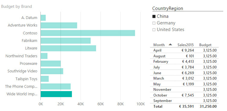
There are two issues with the report in Figure 4-24:

• Sales for January and December are missing from the tabular data. This is because there are no sales in January and December, so the corresponding rows are missing. This is a big issue, because the budget is computed as the total budget divided by 12, but only 10 rows are accounted for in the final figures. As a result, the budget values of the reports are wrong. In fact, the budget for World Wide Importers in 2016 was 37,500, whereas the report shows a total of only 31,250.

• While searching for the missing months, you might have noticed that months are not sorted in sequential order. In fact, by default, Power BI sorts each column alphabetically, which, of course, is not the correct way to sort months.

David is determined to solve these two issues, beginning with the last one, which is somewhat easier. To sort the months by sequential order, he needs a new column in the Sales table containing a number, ranging from 1 to 12, which contains the sort order of the month. The problem is there is no such column available, and there is no predefined functionality to achieve this goal.

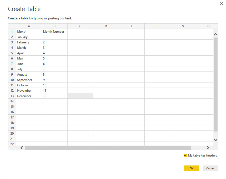
If David’s data were still in Excel, he could easily add the column to the table manually, but now data is coming from SQL Server, in the Contoso database, and he cannot modify the content of the SQL Server view to show such a month. Fortunately, Power BI Desktop offers you a great feature when you have some data to add to an existing model: you simply enter it. To do this, on the Query Editor ribbon, on the Home tab, in the New Query group, click Enter Data, and Query Editor shows you a grid in the Create Table dialog box, in which you can type (or paste) the data you want to add to the model. Figure 4-25 shows how David used this feature to create a table containing the month names and numbers.

The next step, after saving and renaming the table as Month Numbers, is to bring the Month Number column from this table into Sales 2015. The technique you use is very similar to what David already did with the budget: join the Sales 2015 table with Month Numbers. This time, the relationship is based on the month name. Figure 4-26 presents the Merge dialog box already prepared.

After the merge, you still need to expand the Month Number column and load the content in the Power BI Desktop data model, similar to what you did in back in Figure 4-15.

Now that the month number belongs to the table, you need to instruct Power BI to sort the month names by month number. In the Fields pane, click the month name. Note that the ribbon displays a new tab: Modeling. On the Modeling tab, click Sort By Column (number 1 in Figure 4-27), and then select Month Number (number 2 in Figure 4-27).

After you select it, the report changes and shows the months correctly sorted, as demonstrated in Figure 4-28.

Now that David has the months displaying correctly, it is much clearer that January and December are missing, so he turns his attention to fix this. Because this requires a bit more work, there needs to be a bit of fore planning.

First, David needs to decide which year to use as a basis for demonstrating seasonality. In fact, Wide World Importers might have sales in January 2014 and no sales in January 2015. Should he consider 2014 or 2015 to decide what to allocate in January? David goes for 2015 because it shows the best figures. You might make different decisions here, but as we have cautioned several times already, keep in mind that this is a book about Power BI, not a budgeting tutorial. So, please be patient; we are very naïve regarding choices like this one.

Now that David has made his decision, he needs to build a table containing, for each country/region and brand, the number of months for which there are sales in 2015.

This requires several steps in Query Editor:

1. Start from Sales 2015, and then remove all the unwanted columns, to keep only CountryRegion, Brand, Month, and Sales2015.

2. Remove all the rows in Sales 2015 that are empty.

3. Remove the Sales2015 column.

4. For each brand, count the number of months.

The first part of step 1 is easy: in Query Editor, right-click Sales 2015, and then, on the shortcut menu, click Duplicate to make a copy of the table. Name the copy Months Count.

The second part of step 1 is also easy: using the small delete icon that appears in the applied steps of the Query Settings panel (see Figure 4-29), remove all of the steps, keeping only the first two (Source and Navigation), so as to return to the original query.

Remember, we are working on a copy of Sales 2015, so we are free to update it as needed. The original table remains untouched.

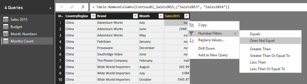
At this point, you can delete the two Sales2013 and Sales2014 columns, which are not needed for the purpose of this query. To do this, right-click the column header for each column and then, on the shortcut menu, click Remove Columns. Step 1 is done!

Moving on to step 2: David notices that the first row (China, Adventure Works, July) contains a null value for Sales2015. He right-clicks the value to open its shortcut menu, where he chooses Number Filters and then Does Not Equal, meaning that he wants to filter only the rows for which Sales2015 is not null, as shown in Figure 4-30.

Step 3: At this point, the column Sales2015 is no longer useful; David can remove it as he did with the other two years. Steps 2 and 3 are now also done, in just a few clicks.

Finally, step 4: Group the current dataset by CountryRegion and Brand, then count, for each combination, the number of months. Because this is a very common operation on datasets, Query Editor offers a specific functionality: first, select the columns to group by, and then choose Group By, as illustrated in Figure 4-31.

You use the Group By dialog box to choose the columns to group and the operation to perform on other columns. In this case, the default options are good (see Figure 4-32): David wants to group by CountryRegion and Brand, and then count the number of rows (which is, months) for each combination.

After he clicks OK to confirm this dialog box, David sees the dataset shown in Figure 4-33.

Now, the new dataset indicates how many months are present for each brand and country/region. You need to use this number, instead of 12, in the division of the budget to obtain the correct value to use for each month. Of course, you do not want this table in the model, so you turn off loading for it. This table is considered a helper table: you will use it with a join operation with Sales 2015. The table contains information that is useful only during the join operation, but not beyond that.

Thus, the last step is to modify Sales 2015 to take this number into account. This time, you do not need to add further steps to an existing query; however, you need to replace some of them, and this requires a bit more attention.

If you reopen the Sales 2015 query in Query Editor and begin navigating through the Applied Steps panel, you notice that what is displayed in the results pane reflects what the query looks like after having applied the selected step. For example, in Figure 4-34 you can see that when you select the Added Custom step, the query shows the Budget 2016 column, which will be removed by the next step.

You need to add a few steps before the Added Custom step (which computes the Budget, divided by 12) and then modify the calculation of the budget itself. When you choose an operation from the toolbar, the step is added right after the currently selected one. Thus, you select the fourth step (Expanded NewColumn) and, there, you add the merge of Sales 2015 with Months Count, basing the relationship on CountryRegion and Brand.

Figure 4-35 presents the Merge dialog box for the inclusion of the Number Of Months column.

After you add the column to the view, you must replace the expression for the Budget 2016 column with a different one. In fact, you want to compute the Budget 2016 column divided by the number of months, for only the months for which there are sales in 2015. To perform this operation, in the Applied Steps area of the Query Settings pane, click the settings button (the small “gear” icon) to the right of the Added Custom step, and then change the expression accordingly, so that it appears like that shown in Figure 4-36.

With the new query in place, the report is updated as soon as you click OK, and now it shows correct figures, as demonstrated in Figure 4-37.

Here are the most relevant features:

• Power BI Desktop can load data from any database. In the example in this chapter, we used Microsoft SQL Server.

• Using Power BI Desktop, you can load data from multiple sources. In the example, we mixed data from Excel with data residing in a SQL Server database.

• Power BI Desktop uses Query Editor to load data. Query Editor offers many powerful features. We highlighted in particular the capability of merging different queries and adding calculations to the query.

• Some queries are loaded into the model; others are useful only to compute values in the main query. You can mark queries that should not go into the model as “do not load” so that they are used only in Query Editor.

• You can upload a Power BI Desktop model to the Power BI online service, and it retains the same refresh features: by using the Personal Gateway, you can refresh a Power BI model in the cloud, letting it access data on your PC.

At the beginning, it might look complex, but after you get used to it, Query Editor offers you a lot of power to build your models. Having successfully finished this chapter, you can call yourself a data modeler. Later in the book, we will introduce some more features of Power BI Desktop to further enhance your model with more advanced calculations.