This chapter covers an agriculture industry-based case study for predicting a cash crop yield. The case study gives you an idea of the challenges faced by a mid-sized agri-conglomerate trying to reach the next level and become as big as the vision of its founder. The problem of crop yield is very important for such organizations due to the fact that they want to maximize their land resources to get the highest revenue possible. What you will primarily learn in the case study is the fact that a company’s vision should be tied to the machine learning operation that it is undertaking; otherwise it will be a wasteful expenditure. This is what I tell most of my clients when they hire me for consultation to look at how their current machine learning application helps them. Does it lower costs? If so, by how much to increase revenue? Then by how much? The goal of the project has to be quantifiable or it will not be successful but it will give dissatisfaction to the business owners and stakeholders. So read on…
Agriculture Industry Case Study Overview
Global Yearly Production at Aystasaga Agro for Three Cash Crops
Aystsaga Agro | ||
|---|---|---|
2017-2018 Worldwide Production | Tonnes | Total Land Size |
Sugarcane | 470817.99 | 5361.70 |
Sugar beet | 503999.80 | 5361.70 |
Tomatoes | 273446.70 | 5361.70 |
In 2013, Aystsaga Agro purchased big farms in Brazil and South Africa. The Brazil farms were in the region of Sao Palo, and the South African farms were in the interior regions. Tamio, the founder of the company, succeeded in expanding the company’s agriculture farming operations by acquiring land and using it for commercial operations. His vision was to establish his company as a major agri-business in the world.
Worldwide Production Numbers and Revenue Figures for Aystsaga Agro
2017-2018 Worldwide Production | Tonnes | Total Land Size | US$ |
|---|---|---|---|
Sugarcane | 470817.99 | 5361.70 | 241058809.3 |
Sugar beet | 503999.80 | 5361.70 | 25199990 |
Tomatoes | 178446.70 | 5361.70 | 180231167 |
Income from Agricultural Operation | 446489966.3 |
While he was looking at the numbers, there was a knock on his plush South African office cabin door. He raised his head to catch his Chief Operations Officer, Glanzo, smiling. He signaled for him to come and sit in front of him. As Glanzo came and sat down, Tanio rose up and went near the right side of the window. He looked at the breathtaking view of the sea in the South African capital as he started speaking slowly.
The Problem
“Have you seen the numbers sent by Nambi this morning?” asked Tamio.
Glanzo nodded and said, “I think they are pretty impressive given that we have had several storms around our farms in Brazil and South Africa this year.”
“You don’t understand my vision, do you?” asked Tamio, looking straight at his right-hand man. “My vision is to achieve a turnover of USD 500 million and reach USD 1 billion in six years. I told the board about this in the last AGM. You were there too,” said the boss.
Glanzo said, raising his shoulders, “We were all there, but I thought you were saying that to please the investors and the board.”
“No, that was a goal that I have been working towards for the past 15 years, ever since this company went public. This is not just a vision or a goal; this is a challenge that I have thrown up to you all,” said Tamio decidedly.
Glanzo retorted, “Yes, I understand the need to grow; otherwise, we will be eaten by the big fish in the industry. But you must understand the challenges that our operations are facing today, and unless we find real solutions for them, we will not grow at the rate that you want it to happen.”
Tamio now had a frown at his face as he sat down and rested his head on his huge, leather executive chair. He was listening intently as Glanzo spoke further. “The single thing that is preventing us from growing is our ability to predict the yield of crops in a given land.” Glanzo continued, “Our agriculture operations are a major problem for us in regions where we made a bad decision in buying infertile land that is low yielding. Low yielding land requires us to rectify it by applying different chemicals on hectares of land, which increases the cost of production and eats into our profitability. If we have to grow at the rate that you are spelling out, we need a way to determine which land is high yielding for a particular crop. If we are able to achieve this, we can avoid buying farms that are unproductive and low yielding, like the ones we have in Brazil where the soil is highly acidic and has to be treated with lime to make it more alkaline.”
Tamio raised his head slightly, signaling that he understood what Glanzo was talking about. He asked, “Do you know of a way to find out how to predict the yield for a particular type of land, Glanzo?”
Glanzo responded, “I have been looking at some of the research that has been happening in universities around the world; however, nothing concrete is available. But, in my opinion, data machine learning and AI show some promise to solve the problem. We can hire some machine learning engineers and data scientists who can help us create a model for ascertaining the yield of crop in a particular land location.”
“That sounds great. Why don’t you form a team to look into this problem and propose possible solutions?” asked Tamio, smiling at Glanzo.
Glanzo said, “Yes, that is what I intend to do. First, I’ll hire machine learning engineers and data scientist and then I’ll add people from our business operations to the team.”
“Send me an email for approval to go ahead,” said Tamio, picking up the eyeglasses from his desk as Glanzo rose to leave his cabin.
Machine Learning to the Rescue?
The machine learning team was formed in two months’ time with Hert Liu hired as the machine learning engineer for the pilot project. Along with three data scientists, he was made to take a robust tour of Aystsaga Agro’s agriculture operations in Brazil, South Africa, and India. The business operations team members were introduced to them once their induction program was over. With detailed briefings, Hert and his team had various new words typical to agriculture farming added to their vocabulary. They also understood the inside processes that went into producing crops. The detailed tours really helped the team in dig deeper into the company’s operations. However, what they lacked was the experiential knowledge, and that is the gap the business operations team members were going to fill in this pilot team.
Hert and his team met a couple of times after coming together. They met Glanzo several times too. He effectively communicated the company founder’s vision and the problem at hand, which was linked to its growth. Hert was an experienced machine learning engineer who worked in the insurance domain earlier. His only brush with agriculture was creating a model for predicting claims for agricultural farmers. So this was a very high learning curve for him, where he had to understand the intricacies of the commercial farming business and also the intricacies involved in managing it, such as crop failures due to insect infestations, changes in weather patterns, and the soil constitution and its effects on farm output. Hert and his team started gathering some parameters that they felt could help in predicting the farm output of a crop. They divided their analysis into weather, soil, and economic environments. They shared their understanding with Glanzo in bi-weekly meeting with him. Hert showed how weather was damaging crops in their Indian farms due to unpredictable rains and floods near the farm. Glanzo pointed out that the biggest problem they faced was determining the profile of high yielding farm land before purchase. “As per our founder’s vision, we are looking to buy a lot of farm land around the world such as in Australia, Thailand, and other regions; however, we can’t do this simply by blindly buying land and then finding out it yields less crop that the average farming operations. This means disaster to our ROI. You as a team should build a model that helps us in determining the profile of high yield cash crop farmland. To do so, you should look at the soil profile and what makes soil give high yield or low yield. Use whatever instruments you want; we can buy them. There is no shortage of funds but you must build a system that will benefit us the most in our bid to grow exponentially,” he said.
Parameters for Monitoring Soil Nutrients
Soil pH |
|---|
Organic Carbon % |
Nitrogen kg/ha |
Phosphorus kg/ha |
Potassium kg/ha |
Zinc mg/kg |
Iron mg/kg |
Copper mg/kg |
Manganese mg/kg |
Sulphur kg/ha |
- 1.
Commercial grade IoT sensors kits to read soil nutrient data
- 2.
Soil nutrient manual testing kits for places where IoT sensors were hard to run
We are now going to build a solution for the problem of predicting the yield of a sugarcane cash crop based on the dataset from the file cashcrop_Yield_dataset.csv.
Solution
We can assume that the dataset is produced after reading soil samples from the IoT sensors and manual soil nutrient test kits for the various parameters given in the dataset file cashcrop_Yield_dataset.csv . The code in Listing 9-1 is not the most definitive solution for this problem but one that is simple and quick to achieve, as in any pilot project. In a real-world scenario, the data collected for soil nutrients will have many more parameters. Such a data collection exercise may take months to complete if the size of operations spans several continents. Agriculture operations are spread far and wide away from urban places so it’s a hectic job for any company to comply. We’ll keep these factors in mind when designing a solution. Note that we’re only using linear regression as it gives a highly accurate score; however, I leave it up to you to try other regressor algorithms.
The Python Code
Code for the Solution of the Case Study
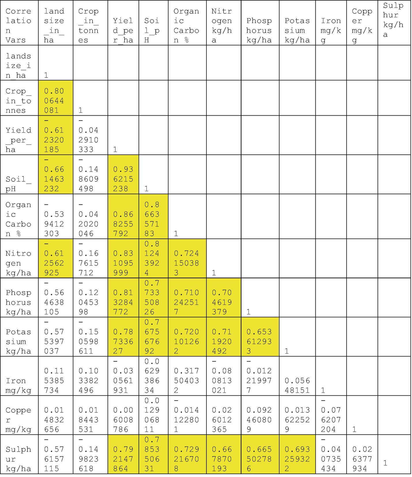
Correlation between the variables
Soil_pH
Organic Carbon %
Nitrogen kg/ha
Phosphorus kg/ha
Potassium kg/ha
Sulphur kg/ha
Output of Code from Listing 9-1

Vertical boxplot visualization

Horizontal boxplot visualization

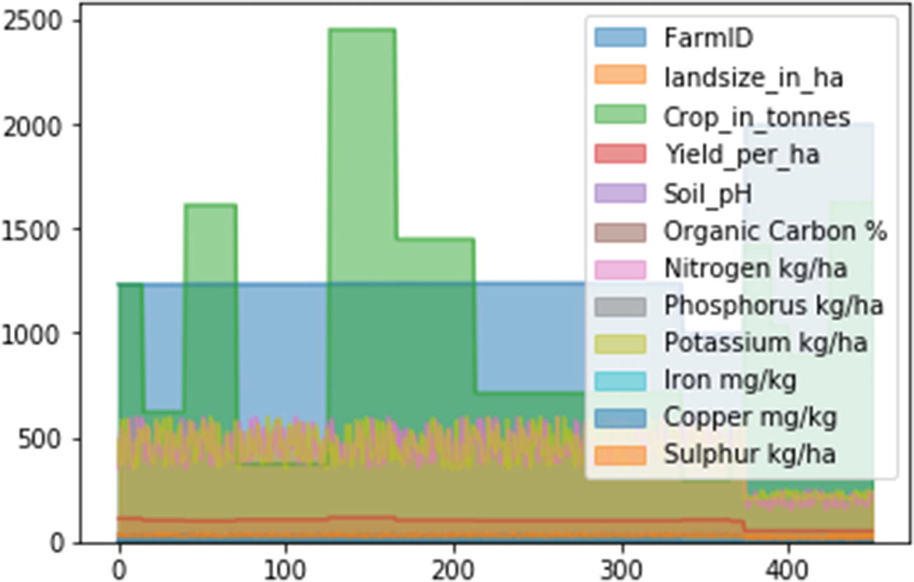
Area graph of the numeric variables

Histogram of the numeric variables

Stacked area plot of the numeric variables
Cumulative stacked area graph

Scatter plot of Yield_per_ha and Soil_oH variables

Chart plot of Yield_per_ha and Soil_oH variables
In Figures 9-2 through 9-8, we can see that the bloxplot shows us a highly distributed value of Crop_in_tonnes. One way to avoid seeing this is to apply scaling to all of the numerical variables, like I did in the case study solutions for healthcare, retail, and finance in my book Machine Learning Applications Using Python. The histogram shows the distribution of variables, and we see that most of the soil nutrients are right-skewed except for copper and iron. We also note that the scatter plots for Yield_per_ha and Soil_pH are closely related through the Python code df.plot.hexbin(x='Yield_per_ha', y="Soil_pH", gridsize=20). After completing the usual data preparation steps by dividing it into a target variable named cropyield and a features variable with all the other features, we then split the dataset into training and testing datasets with 360 samples belonging to the training dataset and 91 samples belonging to the testing dataset. After this, we load the linear_model Python library to execute the linear regression algorithm on the training and testing datasets through the Python code regr.fit(X_train,y_train) , y_pred= regr.predict(X_test). Then we look at the accuracy score that we get with our testing dataset before starting to make a prediction through the code print("Variance score: %2f" % r2_score(y_test, y_pred)), which gives us 0.9502, or 95.02% accuracy. Since this is good, we can proceed with making a prediction. Please remember that this is fictitious data so we are able to achieve a good accuracy level. However, in the real world, you may need to run more regressors or fine-tune your data gathering efforts in order to achieve such an accuracy level.
Predicted Value by the Python Program
Please remember that this program does not take into account other conditions such as weather and seed varieties, which also effect crop production and yield. Building such a dataset would definitely be a huge exercise beyond the scope of this book.
Summary
We have now come to the end of this case study and the book. I have thoroughly enjoyed bringing you these IoT-based solutions to modern-day, practical business problems and trying to solve them through machine learning. I hope you enjoyed learning from them too. Do consider leaving feedback on the forums at www.pmauthor.com/raspbian.