Chapter 4: Computer Systems

As we discussed in previous chapters, a digital forensic investigator must be able to control the environment in which they operate. The diversity of computer hardware, operating systems, and filesystems requires the digital forensic investigator to have a firm understanding of all the different and potential configurations they may encounter. This requires the digital forensic investigator to have procedures or controls in place to protect the integrity of the digital evidence and the processes used to examine it. If you do not understand the boot process and how the system reacts when it starts or which filesystem is in use on the storage devices, you could make a fatal mistake. You have to understand how they work together. Failure to understand these basic components could lead you to alter the digital evidence. You will also find that you will be less effective when you testify in judicial or administrative proceedings.

In this chapter, we will cover the following topics:

• Understanding the boot process
• Understanding filesystems
• Understanding the NTFS filesystem

Understanding the boot process

In order to control the environment as we start our investigation, we must understand the environment. Here, digital evidence is being stored, created, and accessed. In most cases, this will be a computer system. I use the term "computer system," and what that comprises is the operating system, the filesystem, and the hardware bundled together to create a computer. To be effective, you must understand the physical media the data is stored on, the filesystem used on the storage device, and how that data is tracked and accessed while on the storage device. Once you understand the process, you can then implement controls to protect the integrity of the digital evidence.

So, what is the boot process? Well, when you push the power button and electricity energizes the system, a series of commands is issued. As it executes the commands, the system is taking steps (just like on a ladder) to achieve the goal of a running operating system. If something breaks any of those steps, then the system will not load.

The first step is the Power-On Self-Test (POST); the CPU will access the Read-Only Memory (ROM) and the Basic Input/Output System (BIOS) and test essential motherboard functions. This is where you hear the beep sound when you turn the power on to the computer system. If there is an error, then the system will notify you of the error through the use of beep codes. If you do not have the motherboard manual, do a search to determine the meaning of the specific beep code.

Once the POST test has successfully completed, the BIOS is activated and executed. Note that the system has not accessed the storage media. All the program executions are taking place at the motherboard level and not in the storage devices. The user can access the BIOS by using the correct key combination as it is displayed on the screen.

Note

The time allowed for you to hit the correct key can sometimes be quite short. If you are unsuccessful, the system will continue booting and will access the storage device. If you are trying to access the suspect's computer system, disengage the storage devices if they are accessible before starting the process. This will ensure that you are not booting to the suspect's storage device and destroying evidence.

The BIOS will have the basic information of the system: the amount of RAM, the type of CPU, information about the attached drives, and the system date and time. The easiest way to document this information is to take a photograph of it as it is displayed on the screen. This is also where you can change the boot sequence. Typically, the system checks the CD/DVD first and then the designated hard drive. This is where you would be able to change the setting of the boot device when we create the boot media later on in the chapter. Changing the boot device tells the BIOS to access the device we are providing, and not the suspect's.

In 2010, the BIOS function was replaced by the Unified Extensible Firmware Interface (UEFI). It provides the same service as the BIOS, but has been enhanced, as follows:

• By providing better security at the pre-boot process
• Faster startup
• Will support drives larger than 2 TB
• Support for 64-bit device drivers
• Support for the GUID partition table (GPT)

The Secure Boot feature allows us to use authenticated operating systems when booting the computer system. This can be an issue if you are attempting to use an alternative booting device.

As you can see in the following diagram, once the power is turned on and it has completed the POST test, depending on the system, it may boot with the BIOS, or it may boot with the UEFI scheme:

Figure 4.1 – Boot process

The BIOS will look for the Master Boot Record (MBR) of the boot device. The MBR is located at sector zero and holds information about the partitions, filesystems, and the boot loader code for the installed operating system. Once the MBR is found in the boot loader and has been activated, control is then passed over to the operating system to complete the booting process.

The UEFI will look for the GPT; the GPT will have a protective MBR to ensure legacy systems will not mistakenly read this as being unpartitioned and overwrite the data. It will also contain the partition entries and backup partition table header. A GPT disk can contain up to 128 partitions for a Windows operating system. Just like in the BIOS scheme, once the active partition and boot loader have been found, the operating system will take over the booting process.

Since you now understand the boot process, we still want to control the boot environment with the creation of forensic boot media, which we will discuss next. 

Forensic boot media

It is a widespread practice to remove the hard drive from the system to create a forensic image. However, sometimes, the storage device cannot be removed from the system, and you have to create a forensic image. To accomplish this task, you need to use a bootable CD/DVD or USB device to create a forensic environment in order to create a forensic image.

Using boot media, you will want to ensure that it will create that sound forensic environment and not cause any changes to the source device. As we discussed during the boot process, we want to intercept any potential changes to that source device, and we want to have the system boot inside an environment we control. While it is still possible to boot using a CD/DVD, it is becoming more common to find systems without an optical drive. Without an optical drive, we must use a boot USB device to create a sound forensic environment to access the storage device.

Linux is a standard operating system that has been used to create a USB-based (live) operating system to create the forensic environment needed to examine these devices. As discussed in Chapter 3, Acquisition of Evidence, Paladin is one such tool. It is freely available to download and to purchase if you wish to have it preinstalled on a USB device. Sumuri also provides some limited technical support in the operation of Paladin.

There is also a Windows-based bootable environment known as WinFE (Windows Forensic Environment). WinFE was developed by Troy Larson in 2008 and has spawned other tools such as Mini-WinFE, which was developed by Brett Shavers and Misty (http://reboot.pro/files/file/375-mini-winfe/). The benefit of using the Windows bootable environment is that you now have access to Windows-based forensic tools. It is possible to run X-Ways or FTK Imager from this secure environment. I would not recommend using a tool that is resource-heavy. What I mean by this is that some forensic suites such as EnCase Forensic or FTK require significant resources to run effectively. X-Ways can be run from a USB device, as can some artifact-specific tools such as RegRipper. 

As with any tool or procedure, you must validate it to ensure you are getting the expected results. This means that before you go out into the field and boot a suspect's computer utilizing a forensic USB device, you must test it in the laboratory environment to ensure no changes are made. Some of the challenges that you, as the examiner, need to be concerned with when using a bootable USB device include the following:

• Ensuring the system will boot to the device and not the internal hard drive by changing the boot order in the BIOS.
• In some systems, it's difficult to access the BIOS in the time provided during the boot process.
• Ensure the system can boot to a USB device – some older systems cannot.
• Knowing which filesystems the bootable device can write-protect and which ones it cannot.
• Dealing with the secure boot feature of the UEFI boot process.

As mentioned earlier, secure boot is a security feature of the UEFI process that allows trusted software to boot the system. If we want to use a bootable forensic operating system, the secure boot feature must be disabled.

You must enter the UEFI environment by pressing the catch key such as F2 or F12 (this will vary depending on the computer manufacturer). Once you have entered the setup utility, navigate to the Security menu (this might also vary depending on the computer manufacturer) and disable the secure boot option. Some Linux distributions and WinFE have received signed status and will boot a system that has secure boot enabled.

You must document your steps as you go through this process. If you miss hitting the catch key and start the boot process in the host operating system, then you must document that it occurred. Even starting a partial boot will change the timestamps and make entries in various logs in the operating system.

Now that you understand what a bootable forensic device is, let's go ahead and create one in the next section. 

Creating a bootable forensic device

To create a bootable forensic device, you will need a USB (I recommend using an 8-GB, or larger, device) and an ISO file for the operating system you wish to install. I will demonstrate using an ISO for Paladin and free software called Rufus (https:/rufus.ie/). Rufus is a utility used to create bootable USB devices.

Once you download Rufus, execute the executable and the program will run:

Figure 4.2 – Rufus

Something similar to the preceding screenshot (Rufus) will appear, and you will have to select the appropriate choice from the drop-down menus:

• Device: This is the destination. It is the USB device you want to host the bootable operating system.
• Boot selection: This will be the "live" operating system. Here, I am using an ISO file for Paladin 7.04.
• Partition scheme: You have a choice of using MBR or GPT. Using MBR will give you greater flexibility in the devices you can boot.
• Target system: With the MBR selection for the partition scheme, you can use the device on either a BIOS or UEFI system. If you select GPT for the partition scheme, you can only target UEFI systems.

Under Format Options, accept the default values and then click on the START button. Once the program completes, you will have a fully functioning, bootable forensic environment.

We have created a forensic boot environment; let's discuss the storage media you will encounter. We will now discuss hard drives. 

Hard drives

The term "physical drive storage device" refers to the hard disk drive itself. That is, a physical device that contains platters or solid state storage that holds data. The term "logical device/volume/partition" refers to the formatting of the physical device. A physical device can contain one or more logical devices/volumes/partitions. It is a common misconception that the term "C drive" refers to the physical device, when, in actuality, it refers to a logical partition on the physical device.

Several components make up the interior of the hard drive (as shown in the following figure). If you were to open the case, you would find the hard drive comprised one or more platters. There could be one or more platters stacked together with a spindle in the center. The platters, which are made of a metal alloy or glass, are coated with a magnetic substance in which the heads magnetically encode information on the platters. The heads can write data on both sides of the platter. The spindles of the hard disk cause the disks to rotate at thousands of revolutions per minute; the faster the spindle causes the platters to spin, the higher the efficiency of accessing the data encoded on the platters. To read or write data to the platters, the heads are positioned less than .1 microns from the surface of the platter. Additionally, the actuator controls the heads; it swings across the platter, placing the head in the correct position to read/write the data. The storage devices are manufactured with tight tolerances and can be damaged by sudden sharp movement or a mechanical shock:

Figure 4.3 – Hard drive

A hard drive can have different interfaces, for example, you may run into some of the following:

• Small Computer System Interface (SCSI): An older standard that is typically seen in the corporate environment. Limited to 16 chained devices and will have a terminator at the end of the chain.
• Integrated Drive Electronics (IDE/EIDE): An older standard, but may still be found in older consumer computer systems.
• Serial Advanced Technology Attachment (SATA): A current standard found in many consumer and commercial environments.
• Serial Attached SCSI (SAS): A current standard that is typically found in commercial environments.

Solid state drives (SSDs) are storage devices that contained no moving parts. Instead, they are made up of memory chips. As we discussed earlier, a traditional hard drive has several moving parts in which to read/write data to the spinning platters. With an SSD storage device, all of the data is stored in memory chips, allowing for the following:

• Less weight
• Increased reliability
• Improved data access speed
• Reduced power consumption

For an SSD to function reliably, there are several operations controlled by the firmware of the device. We know these functions as follows:

• Wear leveling: This spreads the writes across the different chips so that it uses the chips at the same rate.
• Trim: This will wipe the unallocated space of the device.
• Garbage collection: As the firmware scans the memory modules, it may identify pages within the data blocks that have been deleted. The firmware will move the allocated pages to a new block and will wipe the data block so that it can reuse the blocks. The firmware can only delete data in blocks.

The real-world effect on forensics is that we can no longer recover data that is, or was, in unallocated space. Since these operations are conducted at the firmware layer, as soon as we give power to the device, these operations start automatically. Currently, there is no way to stop the firmware from doing the functions mentioned previously.

The drive geometry of a platter drive details how data is stored on the device; the drive geometry defines the number of heads, the number of tracks, the cylinders, and the sectors per track. The manufacturer performs what it refers to as a low-level format, which creates the basic structure of the disk by defining the sectors and tracks. A track is a circular path on the surface of the platter, as indicated in the following diagram. The red circle (A) is a single track and each side of the platter will have its own set of tracks. They then subdivide the track into sectors. A sector (B) is the smallest storage unit on the device. Originally, a sector used to be 512 bytes in size; however, newer disks are being formatted with a sector size of 4,096 bytes:  

Figure 4.4 – Drive diagram

The platters have an addressing scheme so that they can locate the data; originally, Cylinder, Head, Sector (CHS) was used. Here, Cylinder refers to the vertical axis of the same sectors on all the platters. Head refers to the read/write heads; each platter has two heads. And, in this case, Sector refers to the number of sectors per track. This addressing scheme worked for large capacity hard drives; however, as the storage capacity increased, the CHS scheme could not scale because of file size limitations, so Logical Block Addressing (LBA) was created. With the LBA scheme, you can address the sectors with a sector number starting from zero.

So, we have discussed the physical components of the device. We will now dive deeper and examine some of the internal aspects. 

MBR (Master Boot Record) partitions

Three steps are required before the computer system can use the storage device. We have discussed the low-level format conducted by the manufacturer, but now we will discuss partitioning.

Partitioning occurs when we divide the physical device into logical segments called "volumes." With the MBR partitioning scheme, we are restricted to four primary partitions. With one physical device, you can have a primary partition used to host the Windows operating system, and you can have a second primary partition that hosts a Linux operating system. Note that you must have a primary partition to boot into an operating system. When a user selects the booted operating system, this is known as the active partition.

To get around the partition limit, developers created the extended partition. One of the four partition records is designated as an extended partition, which can then be divided into logical volumes. 

As we discussed previously, we can find the MBR at sector zero. The MBR contains the information needed by the system to boot. The MBR will be contained in sector zero, so it will be no longer than 512 bytes. The partition table will show us which partition is the active partition. Once the starting sector or the active partition is located, the boot process will continue:

Figure 4.5 – MBR map

The preceding MBR map depicts sector zero of a hard disk. This is the MBR for the physical disk. The first 440 bytes are highlighted; this is the boot code. The next 4 bytes are the disk signature and identify the disk to the operating system. The following 64 bytes comprise the partition table. Each 16-byte entry refers to a specific partition. Remember, it restricts us to 4 primary partitions utilizing the MBR partitioning scheme. The final 2 bytes is the signature for the MBR. It identifies the ending of the MBR and will be the last 2 bytes of the sector.

In the following table, I have extracted the four partition tables and reformatted the hex values for easier reading. The first byte will designate which partition is the active partition. A value of x/80 identifies the active bootable partition. A value of x/00 shows the non-active (bootable) partition: 

Figure 4.6 – Partition tables

Typically, you would see the first partition marked as the active partition; in this case, it is the second partition, which is bootable. The next three bytes represent a starting sector for the CHS calculation. So, when we examine the partition table, we can see that the physical device has as a partition of 0 and a partition of 1 with the entries for partition 2 and 3 being zeroed out. This tells us that there are only two partitions on this physical device.

The fifth byte represents the filesystem on the partition. For partition 0, we can see the hex value of DE, which tells us that it is part of the Dell Power Edge Server utilities. Partition 1 has a hex value of 07, which shows the NTFS filesystem. 

If I found the hexadecimal values of 05 or fh, then that would show an extended partition. We would then have to look into the extended boot records of the extended partitions.

Note

You can find a full list of partition identifiers at https://www.win.tue.nl/~aeb/partitions/partition_types-1.html.

The next three bytes are the values for the ending sector of the CHS calculation. The next four bytes show the starting sector of the partition, and the last four bytes show the size of the partition.

The sector values used in the CHS calculation are legacy values for older storage devices. The values showing the start sector and the total number of sectors (partition size) are being used for the current drives using LBA.

Each partition will have a Volume Boot Record (VBR) at sector zero of the partition. The system uses the VBR to boot the operating system in that volume. It is an operating system-specific artifact and is created when the partition is formatted. It will also appear on unpartitioned devices, such as removable media, for example, a USB or floppy disk.

Primary partitions are not the only partitions that you may encounter; you can also encounter an extended partition, which is the subject of the next section. 

Extended partitions

The limitation of the MBR of only allowing four primary partitions resulted in the creation of the extended primary partition. Here, it takes the place of one (and only one) primary partition and enables the user to create additional logical partitions over the four primary partitions.

The following partition map illustrates the replacement of a primary partition with an extended partition:  

Figure 4.7 – Partition map

The following diagram shows the extended partition. Here, the user has created multiple logical partitions within the extended partition boundary:

Figure 4.8 – Extended partition map

The extended partition will not have a VBR. It will have an extended boot record (EBR), which will point to the first extended logical partition. The first extended logical partition will contain information about itself and a pointer to the next extended logical partition. In effect, this will create a daisy chain of pointers from one extended logical partition to the next.

We have now covered the aspects relating to the MBR; let's now go over the GPT formatted aspects. 

GPT partitions

A GUID is a globally unique identifier and uses a 128-bit hexadecimal value to identify different aspects of the computer system uniquely. A GUID comprises five groups and is formatted as 00112233-4455-6677-8899-aabbccddeeff, and, while there is no central authority to ensure uniqueness, it is doubtful that you would get a repeating GUID.

RFC 4122 defines the five different GUIDs as follows:

• Version 1: Date-time and MAC address: The system generates this version using both the current time and client MAC address. This means that if you have a version 1 GUID, you can figure out when it was created by inspecting the timestamp value.
• Version 2: DCE Security: This version isn't explicitly defined in RFC 4122, so it doesn't have to be generated by compliant generators. It is like a version 1 GUID except that the first four bytes of the timestamp are replaced by the user's POSIX UID or GID, and the upper byte of the clock sequence is replaced by either the POSIX UID or GID domain. (UID stands for User Identifier. POSIX stands for Portable Operating System Interface, which is a set of standards to ensure compatibility between operating systems.)
• Version 3: MD5 hash and namespace: This GUID is generated by taking a namespace (for example, a fully qualified domain name) and a name, converts it into bytes, concatenates it, and hashes it. Once it has specified the special bits such as version and variant, it then converts the resulting bytes into hexadecimal form. The special property regarding this version is that the GUIDs generated from the same name in the same namespace will be identical even if they were generated at different times.
• Version 4: Random: The system creates this GUID using random numbers. Of the 128 bits in a GUID, it reserves 6 for special use (version + variant bits) giving us 122 bits that can be filled at random.
• Version 5: SHA-1 hash and namespace: This version is identical to version 3 except that SHA-1 is used in the hashing step in place of MD5.

The GPT is a partitioning scheme that is used for newer storage devices and is part of the new UEFI standard. The UEFI standard replaces the BIOS, while the GPT replaces the MBR partitioning scheme.

The GPT petitioning scheme uses LBA and a protective MBR that can be found in the physical sector zero. The protective MBR allows for some backward compatibility and helps to remove any issues when dealing with legacy utilities that do not recognize the GPT partitioning scheme. There is no boot code available in the protective MBR. As you can see in the following diagram, this is the first partition entry of the partition table of the protective MBR. The partition is identified by hex value EE, which shows it is a GPT partition disk, as shown in the following GPT hex:

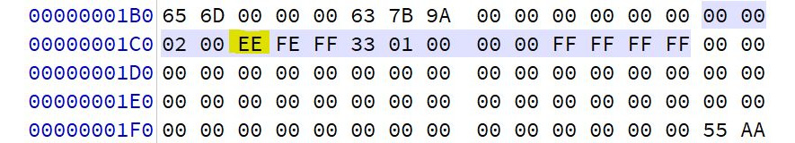
Figure 4.9 – GPT hex

While the MBR contains the partition table within physical sector 0, GPT houses the partition table header at physical sector 1. The GPT header can be identified by the EFI signature of hexadecimal values 45 46 49 20 50 41 52 54, as shown in the following diagram:

Figure 4.10 – EFI PART

The following table shows the layout of the GPT header, which you can use to identify the layout of the desk:

Figure 4.11 – GPT header format

The GPT partition entries are typically found in physical sector 2. The following diagram shows the GPT partition table entries:

Figure 4.12 – GPT sector 2

Each partition entry is 128 bytes and provides information about the partitions. The following table shows the contents of the partition entries, which include the partition type GUID, the GUID that is unique to that specific partition, the starting and ending sectors, and the partition name in Unicode:

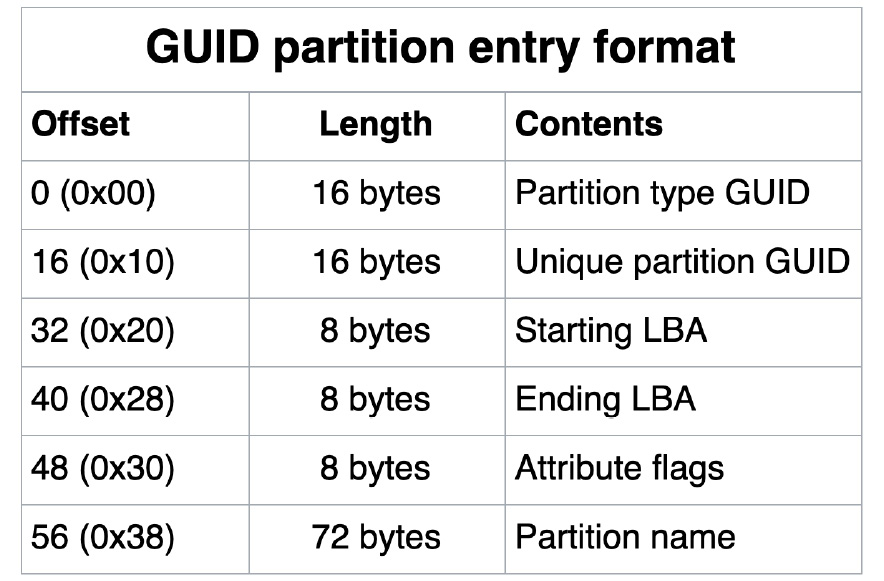
Figure 4.13 – GUID

A partition should hold all of the data on the disk within the partition's boundaries; however, there are spaces on the disk outside of the normal partition boundaries where a technical user may hide data. We will discuss those areas next. 

Host Protected Area (HPA) and Device Configuration Overlays (DCO)

HPA and DCO are hidden areas on the hard drive created by the manufacturers. The HPA is used by the manufacturer to store recovery and diagnostics tools and cannot be changed or accessed by the user. The DCO is an overlay that allows the manufacturer to use standard parts to build different products. It allows the creation of a standard set of sectors on a component to achieve uniformity. For example, the manufacturer might use one set of parts to create a 500-GB hard drive, and while using the same components, can also create a 600-GB hard drive. Once again, usually, the user would not have access to this location. Some utilities to do so are freely available, however, and could be used by a user to access these locations and store data.

The following screenshot shows you how an HPA may appear in X-Ways:

           

Figure 4.14 – HPA 1  

The following screenshot shows you how an HPA may appear in FTK Imager:

     

Figure 4.15 – HPA 2

Let's move on and discuss some potential filesystems that you may encounter. 

Understanding filesystems

A hard drive can have multiple partitions on it, and, in each partition, there will be (in most cases) a filesystem. There might be hundreds of thousands to millions of files contained within a partition. The filesystem tracks where every file is and how much space is available within the partition boundaries.  

We discussed sectors earlier in the Hard drives section, and they are the smallest units that are available to store data. The filesystem stores data based on clusters. Clusters are one or more sectors. A cluster is the smallest allocation unit the filesystem can write to. Now, there are many filesystems available, and some are restricted to specific operating systems unless the user enables drivers that will allow the operating system to read the filesystem. 

We will now look at some of the common filesystems you may encounter.

The FAT filesystem

The File Allocation Table (FAT) filesystem has been around since the early days of home computing, and it is one of the few filesystems that nearly all operating systems can read. It is the de facto standard filesystem for removable devices.

As time has gone by, the FAT filesystem has gone through numerous changes:

• FAT 12: The first version was created in 1977 and used 12 bits (hence, the FAT 12 designation) to address available clusters. This limited its use to only storage devices that could contain 4,096 clusters. It is rarely seen nowadays, but you might find it on a floppy diskette.
• FAT 16: This was created in 1984 and used 16 bits (I see a pattern) to address the available clusters. It had the same issues as the FAT 12, as it could not be scaled to be used with larger capacity devices.
• VFAT: This was introduced with Windows 95 and added the Virtual File Allocation Table. It added the use of the long filename (LFN) and additional timestamps.
• FAT32: This uses 28 bits to address available clusters, theoretically allowing for a maximum volume size of 2.2 TB. Microsoft implemented restrictions that limited the volume size to 32 GB with a maximum file size of 4 GB. It is still in use today and can be found on most removable devices.

We will discuss the FAT32 filesystem for the remainder of this section on the FAT filesystem.

The FAT filesystem is laid out in two areas (as shown in the following diagram, Figure 4.16 – FAT areas):

• System Area: This stores the volume boot record and FAT tables.
• Data Area: This stores the root directory and files:

Figure 4.16 – FAT areas

Next, we will discuss what falls under System Area.

Boot record

In the system area, we have the Volume Boot Record (VBR). We can find it in logical sector 0 (LS 0), which is the first sector within the partition boundaries. The boot process creates the VBR when the partition is formatted and contains information about the volume and boot code to continue the boot process for the operating system. If it is a primary partition, the VBR will consist of several sectors, typically, sectors 0, 1, and 2 with a backup in sectors 6, 7, and 8. The VBR and backups are stored in a "reserve area," which is typically 32 sectors before the first file allocation table begins:

Figure 4.17 – VBR

In the preceding diagram, we can see a volume boot sector, which helps to decipher the following information:

• x00: We will find the jump instructions for the system to continue booting.
• x03: The OEM ID shows which operating system was used to format the device.
• x0B: Bytes per sector.
• x0E: Number of reserve sectors.
• x10: Number of FATs (this should be 2).
• x11: Unused root entries (for FAT32, this should be 0 because the root directory is in the data area).
• x13: Number of sectors (this will be 0 if the number of sectors exceeds 65,536).
• x15: Media descriptor (xF8 will show a hard disk, while xF0 will show a removable device).
• x16: Number of sectors per FAT (for FAT32, this should be 0).
• x18: Number of sectors per track (this should be 63 for hard disks).
• x1A: Number of heads (this should be 255 for hard disks).
• x1C: Number of hidden sectors (the number of hidden sectors before the start of the FAT volume).
• x20: Number of total sectors (that is, the total sectors for the volume).
• x24: Logical sectors per FAT.
• x28: Extended flags. 
• x2A: FAT version.
• x2C: The starting root directory cluster (usually, cluster 2).
• x30: Location of the FS information sector (typically, this is set to 1).
• x32: Location of the backup sector(s) (usually, this is set to 6).
• x34: Reserved (set to 0). 
• x40: Physical drive number (x80 for hard drives).
• x41: Reserved
• x42: Extended boot signature (this should be x29).
• x43: Volume serial number (a 32-bit value is usually generated from the date and time; this can track removable devices).
• x47: Volume label (this might not be accurate; different OSes may not use this field).
• x52: Filesystem type.

Next, we will take a look at the file allocation table.

File allocation table

The next component of the FAT filesystem is the file allocation table, which immediately follows the VBR. By default, there are two file allocation tables (FAT1 and FAT2). FAT2 is a duplicate of FAT1.

The purpose of the file allocation table is to track the clusters and to track which files occupy which clusters. Each cluster is represented within the file allocation table starting with cluster 0. The file allocation table uses 4 bytes (32 bits) per cluster entry. The file allocation table will use the following entries to represent the cluster's current status:

• Unallocated: x0000 0000
• Allocated: The next cluster that is used by the file (for example, it represents cluster 7 as x0700 0000)
• Allocated: The last cluster that is used by the file (xFFFF FFF8)
• Bad cluster: Not available for use (xFFFF FFF7)

A cluster is the smallest allocation unit the filesystem can address. A sector is the smallest allocation unit on the disk. A cluster is made up of one or more sectors. It is very easy to get confused if you comingle those terms. Consider the following cluster example:

Figure 4.18 – Cluster example

As users add files to the data area, the system will update the file allocation table. A file may occupy one or more clusters. Additionally, the clusters may not be sequential, so you could have the data of a file spread in different physical locations on the disk; we typically refer to this as fragmentation.

In the following diagram, we can see a representation of the file allocation table; in this scenario, we have a single file occupying three clusters: Cluster 4, Cluster 5, and Cluster 6. You can see that Cluster 4 is pointing to Cluster 5 and Cluster 5 is pointing to Cluster 6. Cluster 6 has the hexadecimal value for end of file (EOF):

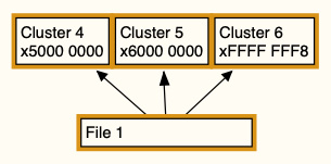
Figure 4.19 – Non-fragmented file entry

In the following diagram, we can see a similar representation of the file allocation table with some changes. We now have two files, with file number 1 occupying clusters 4 and 6. We can see that Cluster 4 is pointing to the next cluster containing the file data, which is Cluster 6. This is an example of file fragmentation. File number 2 is wholly contained within the cluster boundaries of Cluster 5. Cluster 5 will not point to a subsequent cluster; instead, it has the EOF hexadecimal value:

Figure 4.20 – Fragmented file entry

We have covered the system area of the FAT; we will now discuss the data area of the FAT filesystem. 

Data area

The root directory is housed in the data area because, when it was stored in the system area, it was unable to grow enough to work with larger capacity devices. The critical component of the root directory is the directory entry. If there is a file, directory, or subdirectory, then there will be a corresponding directory entry. 

Each directory entry is 32 bytes in length and helps to track the name of the file, starting cluster, and file size in bytes.

In the following diagram, we can see a FAT32 directory with multiple file entries. The filesystem will stop looking for file entries when it runs into a hexadecimal 00, and all values following the hexadecimal 00 will be ignored:

Figure 4.21 – FAT directory entry

In the following FAT directory map, we can see the layout of the directory entry and a short filename (SFN) directory entry with the specific offsets highlighted:

Figure 4.22 – FAT directory map

If the first byte is xE5, then the filesystem will consider that entry as deleted. The remaining bytes of the file or directory name will remain, as will the other metadata.

The short filename must conform to the specifications as follows:

• Eight characters are allowed; if there are less than eight characters, then the name will be padded with x20.
• Three characters are allocated for the file extension (if there are less than three characters, then the name will be padded with x20).
• Spaces and the following characters are not permitted: "+ * , . / : ; < = > ?[]|

The directory entry will always be stored in uppercase. The attribute byte (offset x0B) is considered a packed byte, which means the different values have different meanings.

The following diagram shows that bit values in the Attribute flag can be combined, and the resulting hex value will reflect the combinations. If a file had the READ ONLY flag and the HIDDEN flag, then that would give us a value of 0000 0011, and, when converted to hexadecimal, we get the value of x03:

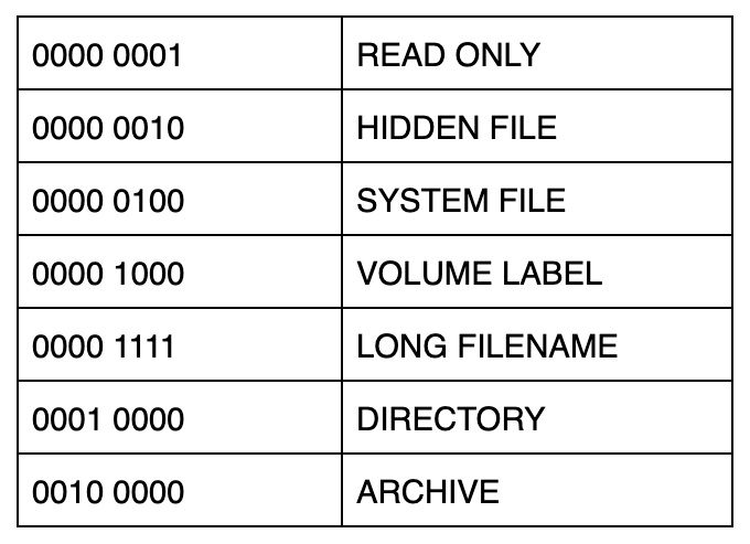
Figure 4.23 – Packed byte

When we look at the example at the bottom of the preceding FAT directory map, we find the hexadecimal value of 20 at the offset x0B; when we convert the hexadecimal into binary, we get 0010 0000. This tells us that the file is an archive.

We can also encounter a Long Filename (LFN); the technique for handling the LFN is a little bit more complicated. We will discuss the LFN in the next section. 

Long filenames

When a user creates an LFN, the system will generate an alias that conforms to the SFN standard. It will format the alias so that the first three characters after the file extension dot will become the extension. The first six characters will be converted to uppercase and will be used for the alias. The alias will then add a ~ character with a following number. It will start with the number 1 and increase incrementally if there are additional files with the same alias name.

The following diagram shows a directory entry for a file with an LFN; the filename is long filename.txt:

Figure 4.24 – LFN

Since this is an LFN, the filesystem will create additional directory entries. In this specific case, there will be two additional directory entries to facilitate the use of the LFN. The first byte of each additional directory entry is the sequence byte. The right nibble is the sequence number. As we look at the directory entry depicted in preceding diagram, the directory entry above the SFN entry has a hexadecimal value of x01. Here, the value of 1 tells us that this is the first value in the sequence. When we move up to the second directory entry, we can see that it has a hexadecimal value of x42, the right nibble informs us this is the second directory entry for this LFN file. The left nibble of the value, 4, tells us this is the last directory entry for the file. In each of the LFN directory entries, you will find that the attribute byte is x0F.

But what happens when a file is deleted? Well, you may be able to recover the file and its associated metadata. In the next section, we will discuss recovering deleted files. 

Recovering deleted files

When a file is deleted in the FAT filesystem, the data itself does not get changed. The first character of the directory entry will change to xE5 and the file allocation table entries are reset to x00. When the filesystem reads the directory entries and encounters xE5, it will skip that entry and start reading from the subsequent entries.

To recover deleted files, we need to reverse the process that the filesystem used to delete the files. Remember, it has not changed the file contents, and they still physically reside in their assigned clusters. We now need to reverse engineer the deletion and recreate the file entry and the entries in the file allocation table. To do this, we need to find the first cluster of the file, the size of the file, and the size of the clusters in the volume.

In the following diagram, we have a directory entry showing us that a file has been deleted. We can see xE5 at the start of the directory entry. (Note that this will require the use of a hex editor to make the changes.)

Then, we have to determine the starting cluster, which is x00 x08 (but is shown as x08 x00 in the diagram). This value is referring to cluster number 8. To determine the file size, take a look at the last four bytes, x27 x00 x00 x00 (remember that the FAT filesystem stores data in little endian, which means the least significant byte is on the left, so we would read that value as x00 x00 x00 x27, and when we convert it into a decimal, we have a value of 39 bytes for the file size):

Figure 4.25 – Deleted entry

Now we have to determine how many sectors make up a cluster and what the sector size is. You will need to go to the boot record to get that information. The boot record shows us that there are 512 bytes per sector, and there are 8 sectors per cluster, which gives us a cluster size of 4,096 bytes (as shown in the following diagram):

Figure 4.26 – Boot record

This means that our file will only occupy a single cluster. We then go to the file allocation table and look at the entry for cluster 8 and see that it is zeroed out:

Figure 4.27 – Deleted FAT

To recover the deleted file, perform the following steps:

1. You need to change the entry in the file allocation table from x0000 0000 to xFFFF FFF8 or xFFFF FF0F. If this were a larger file, you would need to change the file allocation table entry to point to the next cluster until you reach the last cluster and the end of the file size. As you are rechaining the entries, if you come to an entry marked as allocated, when you were expecting to find the entry unallocated, then you may be dealing with a fragmented file. Another alternative is when the clusters were made available for use to the filesystem, a new file was placed in the now-available sectors, which would cause the data to be overwritten. There are not a lot of options available if you run into either one of these situations. If the data is overwritten, then you are stuck. If it is fragmented then you have to try and guess where the next cluster will be, which is not very likely with a large capacity device.
2. The next step is to go back to the directory entry and replace xE5 with another character. When replacing the xE5 character of the filename in the directory entry, be careful to not to guess what the character is. If you select the incorrect character, you could change the meaning or create a bias with the new filename, and that would be improper. I recommend that when recovering a deleted file, you replace that first character with an underscore or a dash so there is no misunderstanding about the filename.

When recovering a file with an LFN, it is important to relink the LFN to the SFN. This is because when the additional directories are created to accommodate the LFN, the system creates a checksum based on the data of the SFN. When you change the xE5 value on the SFN entry, you also want to use the same replacement character for the subsequent xE5 entries for the LFN directory entries. The reason you link the LFN to the SFN is that the SFN directory entry contains information such as the date and time, the starting cluster, and the file size.

It is still possible to recover scraps of data that previously existed on the disk but no longer have any artifacts in the filesystem. This information will be stored in slack space, which is discussed in the next section. 

Slack space

Now is the time to bring up slack space. Remember that the smallest unit the filesystem can write to is a cluster and that clusters are made up of one or more sectors. The reason I keep repeating this is that I have seen people who are new to the field get confused about the difference between the two. The reason this is important is that files come in a variety of sizes; almost no files will conveniently fit within the cluster boundaries. So, you will have files that spill over into the next cluster. The space between the end of the logical file and the cluster boundary is called "file slack." This slack space can contain data from the previous file. Until it is overwritten, that data will remain for you to examine.

You might find evidence of document files, digital images, chat history, or emails; that is, for any data that has been stored on the device, you may find remnants in slack space after the user has deleted the file.

This concludes the FAT filesystems section; next up is NTFS. 

Understanding the NTFS filesystem

The New Technology File System (NTFS) is the default filesystem for Microsoft Windows operating systems. FAT32 had some significant shortcomings, which required a filesystem that was more reliable and efficient, along with additional administrative improvements to help Microsoft remain viable in the corporate environment. They initially designed NTFS for the server environment; however, as the hard drive capacity has increased, it is now the default filesystem in the commercial and consumer market for the Windows operating system.

NTFS is far more complicated than the FAT filesystem; however, the overall purpose remains the same:

• To record the metadata of a file, that is, the filename, the date timestamps, and the file size
• To mark the clusters the file occupies
• To record which clusters are allocated and which clusters are unallocated

The NTFS filesystem comprises the following system files:

Figure 4.28 – NTFS table

To identify a partition with NTFS, we need to look at the MBR or the GPT, depending on which formatting scheme was used. In the following diagram, we can see the MBR for the hard drive and the partition table highlighted after the boot code:

Figure 4.29 – NTFS MBR

Looking at the partition table, we can see that there is a single partition, and, at offset decimal 11 from the start of the partition table, we can see the hexadecimal value of 07. As we discussed earlier in this chapter, this is the filesystem identification for NTFS.

With an NTFS-formatted partition, there is no system or data area like we saw with a FAT-formatted partition. Everything in NTFS is considered a file to include the system data. When we look at the VBR, we can see that it contains information for the system to continue the boot process: 

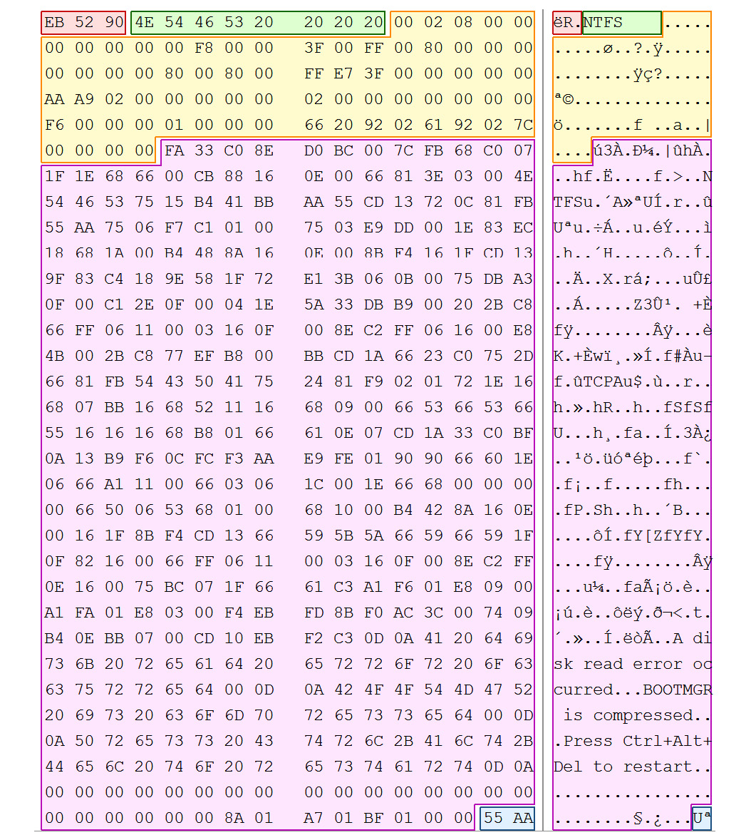
Figure 4.30 – NTFS VBR

The information in the VBR is a file; the $Boot record contains all of the information that we would expect to find in the VBR. The following $Boot diagram shows the data structure for the $Boot file:

Figure 4.31 – $boot

Arguably, the most essential system file in the NTFS filesystem is the $MFT (master file table). The MFT tracks all of the files in the volume to include itself. It tracks each file within the MFT through the use of file entries called a file record. Each file record is uniquely numbered and is 1,024 bytes. Each file record starts with a header, with the ASCII text "FILE", and has an EOF marker of hexadecimal FF FF FF FF. As it adds files to the volume, a new file record is created. If a file has been deleted, the file record will zero out and make it available for reuse. The MFT will look for an empty file record and use it prior to creating a new record. It is possible for the file record to be reused rather quickly, which would overwrite the previous data in the file record. 

As shown in the following NTFS file record example, we can see a file record and file header starting with the ASCII values of FILE. If the record were corrupted or had an error, you would see the ASCII value of BAAD. The file header is 56 bytes:

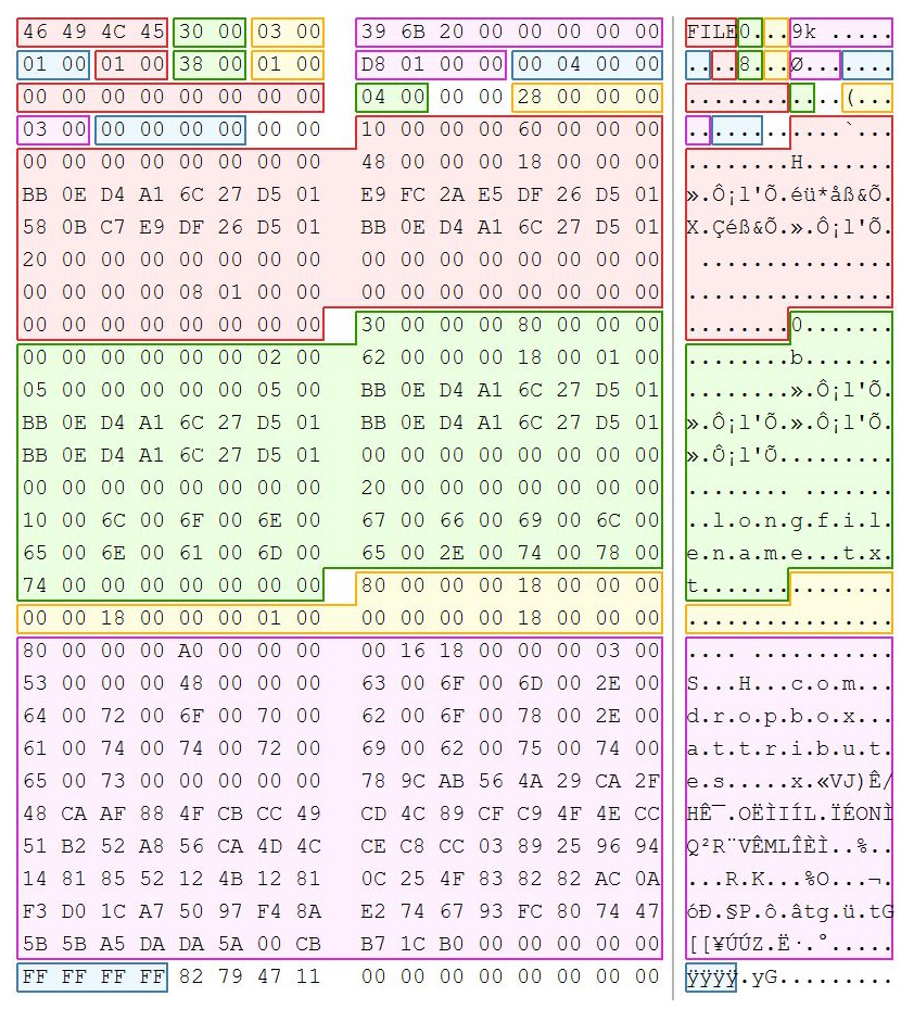
Figure 4.32 – NTFS file record

In the following NTFS file record map, we can see the data structure of a file record header:

Figure 4.33 – NTFS file record map

The file record also contains defined data blocks called file attributes. These store specific types of information about the file. The following file attributes table shows several common file attributes that you are likely to see in almost every record:

 Figure 4.34 – File attributes table

Let's take a look at each of these attributes in detail.

$Standard_Information Attribute (0x10): The file attributes follow the file header and contain information about the file and, sometimes, the actual file itself. The following diagram depicts a file attribute. The first four bytes show the attribute type; in this case, it is the $10 Standard Information Attribute, which contains general information, flags, accessed, written, and created times, the owner, and security ID. It is identified by the hexadecimal header: x/10 00 00 00. The file attribute map contains the decoded values:

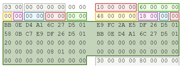
Figure 4.35 – File attribute

Here is a map of the values you will find in the attribute:

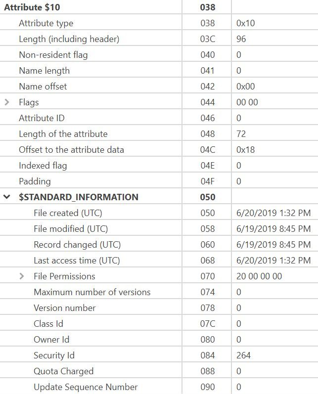
Figure 4.36 – File attribute map

$File_Name Attribute (0x30): The next attribute is the $30 File Name Attribute. This attribute stores the name of the file attribute and is always resident. The maximum filename length is 255 Unicode characters. It is identified by the hexadecimal header of x/ 30 00 00 00:

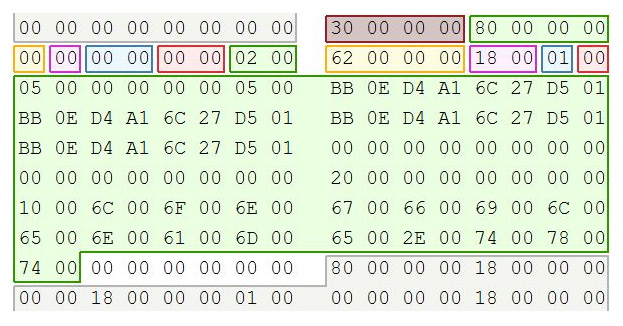
Figure 4.37 – Filename attribute

The following is a map of the values you will find in the attribute:

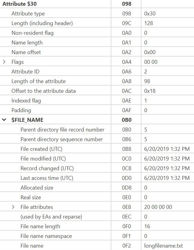
Figure 4.38 – Filename attribute map

$Data Attribute (0x80): The next attribute for this entry is the $80 Data Attribute. The data attribute contains the contents of the file or points to where the contents are located in the volume. This attribute is the file data itself.

If the data attribute content is resident, we only use the attribute header and the resident content header. The resident content of the attribute is the file's data. Only tiny files have a resident data attribute. We will discuss resident versus non-resident data later on in this chapter.

You may find multiple data attributes per file. In this record, the second $80 Data attribute, Dropbox, has added some information to the file:

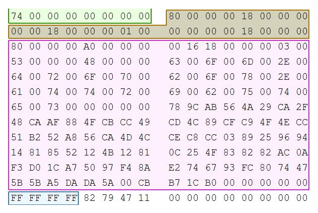
Figure 4.39 – Data attribute

The following is a map of the values you will find in the attribute:

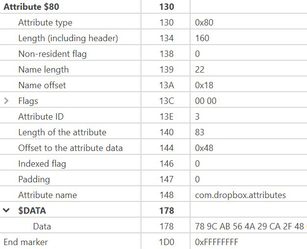
Figure 4.40 – Data attribute map

When examining the $Data Attribute 0x80, the contents of the file may be stored within the MFT file record itself. Since the file record is 1,024 bytes long, it would have to be a tiny file. When the data content of the file fits within the file record, it is called "resident data":

Figure 4.41 – Resident data

In the current example, we have a file named resident.txt that is 23 bytes in size. This is smaller than the 1,024 bytes of the file record. To look at the data of the file, we need to look at the $Data Attribute 0x80 of the file record, as follows:

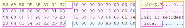
Figure 4.42 – Resident data example

On examining the attribute, we can see the ASCII and hex representation of the file content we observed in the preceding resident data example. When dealing with a non-resident file, such as the one depicted in the following diagram, we can see that the nonresident.txt file, which is 145 KB in size, is larger than the 1,024-byte file record:

Figure 4.43 – Non-resident data

When you look at the $Data Attribute 0x80 of the file, as shown in the preceding diagram, we do not see the contents of the file, but we have pointers to the location of the file within the volume boundaries. We consider this to be non-resident content. Once the content of the attribute becomes non-resident, it can never become resident again. We commonly refer to the pointers in the file record of the attribute as a "run list" for the data runs of the non-resident data:

Figure 4.44 – Non-resident data example

You can have a single data run, or multiple data runs, within the $Data Attribute 0x80. Deciphering the run list for the data runs can be tricky. In the following run list, we have the $Data Attribute 0x80 with two run lists:

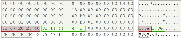
Figure 4.45 – Run list

If the file is not fragmented, then you will have one run list pointing to the data run in the volume. If the file is fragmented (which is very common), then you will have multiple run lists providing information about the starting cluster for each fragment. I have taken the two run lists highlighted in the preceding list and created the following chart:

Figure 4.46 – Run list map

The first run list comprises the hexadecimal values of 31 07 E8 E3 48. Take the first byte of the header (x/31) and add the left and right nibble (3+1=4). 4 is the number of bytes in the run list entry (this is x/07 E8 E3 48). The right nibble (x/1) tells us that 1 byte represents the number of clusters being used for this fragment. We find a value of x/07 in the length field, which represents 7 clusters for this fragment. The left nibble (x/3) informs us that 3 bytes (x/E8 E3 48) will represent the logical starter cluster of the fragment. At the end of the first run, we have a second run list of x/31 14 44 47 17. Like the prior run list, we take the first byte of the header (x/31) and add the left and right nibble (3+1=4). 4 is the number of bytes in the run list entry (which is x/14 44 47 17). The right nibble (x/1) tells us that 1 byte represents the number of clusters being used for this fragment. We find a value of x/14 in the length field, which represents 20 clusters for this fragment. The left nibble (x/3) informs us that 3 bytes (x/44 47 17) will represent the offset from the previous run list cluster. This process will keep going until the system hits x/ 00 00 00 00, which shows the end of the run lists.

That concludes our adventure into the world of NTFS. If you find yourself with a headache, you are not alone! This is just the basics of the filesystem. You can find entire books that have been written about NTFS, if you want to go into much greater detail.

Summary

In this chapter, we looked at how physical disks are constructed and prepared in order to store data. We discussed different partition schemes and how they address the creation of logical partitions. We also learned how filesystems differ and how data is organized.

In the next chapter, we will learn about the computer investigative process and how to analyze timelines, analyze media, and perform string searching for data.

Questions

1. Newer computer systems utilize the BIOS booting method.

   a. True

   b. False

2. A UEFI-based computer system will utilize ____________ to boot from.

   a. MBR

   b. VBR

   c. GPT

   d. LSD

3. A cluster is the smallest storage unit on a hard drive.

   a. True

   b. False

4. An MBR-formatted disk can have more than four primary partitions.

   a. True

   b. False

5. A FAT32-formatted partition is laid out in two areas: a system area and a ___________ area.

   a. Disk

   b. Doughnut

   c. Data

   d. Designer

6. In a FAT32-formatted partition, the root directory is in the system area.

   a. True

   b. False

7. In a NTFS formatted partition, the filename is stored in the _______________ attribute.

   a. Standard information

   b. Filename

   c. Data

   d. Security descriptor

The answers can be found in the rear of the book under Assessment. 

Further reading

Carrier, B. File System Forensic Analysis. Addison-Wesley, Reading, PA., Mar. 2005 (available at https://www.kobo.com/us/en/ebook/file-system-forensic-analysis-1).