11

Machine Learning Pipelines with SageMaker Pipelines

In Chapter 10, Machine Learning Pipelines with Kubeflow on Amazon EKS, we used Kubeflow, Kubernetes, and Amazon EKS to build and run an end-to-end machine learning (ML) pipeline. Here, we were able to automate several steps in the ML process inside a running Kubernetes cluster. If you are wondering whether we can also build ML pipelines using the different features and capabilities of SageMaker, then the quick answer to that would be YES!

In this chapter, we will use SageMaker Pipelines to build and run automated ML workflows. In addition to this, we will demonstrate how we can utilize AWS Lambda functions to deploy trained models to new (or existing) ML inference endpoints during pipeline execution.

That said, in this chapter, we will cover the following topics:

• Diving deeper into SageMaker Pipelines
• Preparing the essential prerequisites
• Running our first pipeline with SageMaker Pipelines
• Creating Lambda functions for deployment
• Testing our ML inference endpoint
• Completing the end-to-end ML pipeline
• Cleaning up
• Recommended strategies and best practices

After completing the hands-on solutions in this chapter, we should be equipped with the skills required to build more complex ML pipelines and workflows on AWS using the different capabilities of Amazon SageMaker!

Technical requirements

Before we start, it is important that we have the following ready:

• A web browser (preferably Chrome or Firefox)
• Access to the AWS account and the SageMaker Studio domain used in the previous chapters of this book
• A text editor (for example, VS Code) on your local machine that we will use for storing and copying string values for later use in this chapter

The Jupyter notebooks, source code, and other files used for each chapter are available in the repository at https://github.com/PacktPublishing/Machine-Learning-Engineering-on-AWS.

Important Note

It is recommended that you use an IAM user with limited permissions instead of the root account when running the examples in this book. If you are just starting out with using AWS, you can proceed with using the root account in the meantime.

Diving deeper into SageMaker Pipelines

Often, data science teams start by performing ML experiments and deployments manually. Once they need to standardize the workflow and enable automated model retraining to refresh the deployed models regularly, these teams would then start considering the use of ML pipelines to automate a portion of their work. In Chapter 6, SageMaker Training and Debugging Solutions, we learned how to use the SageMaker Python SDK to train an ML model. Generally, training an ML model with the SageMaker Python SDK involves running a few lines of code similar to what we have in the following block of code:

estimator = Estimator(...) 
estimator.set_hyperparameters(...)
estimator.fit(...)

What if we wanted to prepare an automated ML pipeline and include this as one of the steps? You would be surprised that all we need to do is add a few lines of code to convert this into a step that can be included in a pipeline! To convert this into a step using SageMaker Pipelines, we simply need to initialize a TrainingStep object similar to what we have in the following block of code:

step_train = TrainingStep(
    name="TrainModel",
    estimator=estimator,
    inputs=...
)

Wow! Isn’t that amazing? This would mean that existing notebooks using the SageMaker Python SDK for manually training and deploying ML models can easily be converted into using SageMaker Pipelines using a few additional lines of code! What about the other steps? We have the following classes, as well:

• ProcessingStep – This is for processing data using SageMaker Processing.
• TuningStep – This is for creating a hyperparameter tuning job using the Automatic Model Tuning capability of SageMaker.
• ModelStep – This is for creating and registering a SageMaker model to the SageMaker Model Registry.
• TransformStep – This is for running inference on a dataset using the Batch Transform capability of SageMaker.
• ConditionStep – This is for the conditional branching support of the execution of pipeline steps.
• CallbackStep – This is for incorporating custom steps not directly available or supported in SageMaker Pipelines.
• LambdaStep – This is for running an AWS Lambda function.

Note

Note that this is not an exhaustive list of steps as there are other steps that can be used for more specific use cases. You can find the complete list of SageMaker Pipeline Steps at https://docs.aws.amazon.com/sagemaker/latest/dg/build-and-manage-steps.html.

In Chapter 4, Serverless Data Management on AWS, we stored and queried our data inside a Redshift cluster and in an Athena table. If we need to directly query data from these data sources, we can use SageMaker Processing right away as it supports reading directly from Amazon Athena and Amazon Redshift (along with Amazon S3). Inside the SageMaker Processing job, we can perform a variety of data preparation and processing steps similar to the transformations performed in Chapter 5, Pragmatic Data Processing and Analysis. However, this time, we will be using scikit-learn, Apache Spark, Framework Processors (to run jobs using ML frameworks such as Hugging Face, MXNet, PyTorch, TensorFlow, and XGBoost), or custom processing containers instead to process and transform our data. Converting this processing job into a step that is part of an automated pipeline is easy, as we just need to prepare the corresponding ProcessingStep object, which will be added later on to the pipeline. Once the processing job completes, it stores the output files in S3, which can then be picked up and processed by a training job or an automatic model tuning job. If we need to convert this into a step, we can create a corresponding TrainingStep object (if we will be running a training job) or a TuningStep object (if we will be running an automatic model tuning job), which would then be added later to the pipeline. What happens after the training (or tuning) job completes? We have the option to store the resulting model inside the SageMaker Model Registry (similar to how we stored ML models in the Registering models to SageMaker Model Registry section in Chapter 8, Model Monitoring and Management Solutions). If we want to convert this into a step, we can create the corresponding ModelStep object that would then be added later to the pipeline, too. Let’s refer to Figure 11.1 to help us visualize how this all works once we’ve prepared the different steps of the pipeline:

Figure 11.1 – Using SageMaker Pipelines

In Figure 11.1, we can see that SageMaker Pipelines provides a bridge to connect and link the different steps that are usually performed separately. Since all the steps in the workflow have been connected using this pipeline, all we need to do is trigger a single pipeline run and all the steps will be executed sequentially. Once all the steps have been defined, we can proceed with initializing and configuring the Pipeline object, which maps to the ML pipeline definition:

pipeline = Pipeline(
    name=...,
    parameters=...,
    steps=[
        ..., 
        step_train,
        ...
    ],
)
# create (or update) the ML pipeline
pipeline.upsert(...)

Then, to run the pipeline, all we need to do is call the start() method:

execution = pipeline.start()

Once the pipeline starts, we would have to wait for all steps to finish executing (one step at a time) or for the pipeline to stop if an error occurs in one of the steps. To debug and troubleshoot running pipelines, we can easily navigate to the SageMaker Resources pane of SageMaker Studio and locate the corresponding pipeline resource. We should see a diagram corresponding to the pipeline execution that is similar to what we have in Figure 11.2.

Figure 11.2 – Pipeline execution

Here, we can see that all steps in the pipeline have been completed successfully, and the model we trained has been registered to the SageMaker Model Registry, too. If we wish to run the pipeline again (for example, using a different input dataset), we can simply trigger another pipeline execution and pass a different pipeline parameter value that points to where the new input dataset is stored. Pretty cool, huh? In addition to this, we can also dive deeper into what’s happening (or what happened) in each of the steps by clicking on the corresponding rounded rectangle of the step we wish to check, and then reviewing the input parameters, the output values, the ML metric values, the hyperparameters used to train the model, and the logs generated during the execution of the step. This allows us to understand what’s happening during the execution of the pipeline and troubleshoot issues when errors are encountered in the middle of a pipeline execution.

So far, we’ve been talking about a relatively simple pipeline involving three or four steps executed sequentially. Additionally, SageMaker Pipelines allows us to build more complex ML pipelines that utilize conditional steps similar to what we have in Figure 11.3:

Figure 11.3 – An ML pipeline with a conditional step

Here, using a ConditionStep, the pipeline checks whether an ML inference endpoint exists already (given the endpoint name) and performs one of the following steps depending on the existence of the endpoint:

• Deploy model to a new endpoint – Using LambdaStep, which maps to an AWS Lambda function that deploys the ML model to a new ML inference endpoint if the endpoint does not exist yet
• Deploy model to an existing endpoint – Using a LambdaStep, which maps to an AWS Lambda function that deploys the ML model to an existing ML inference endpoint if the endpoint already exists (with zero downtime deployment)

Cool right? What’s cooler is that this is the pipeline we will build in this chapter! Building an ML pipeline might seem intimidating at first. However, as long as we iteratively build and test the pipeline and use the right set of tools, we should be able to come up with the ML pipeline we need to automate the manual processes.

Now that we have a better understanding of how SageMaker Pipelines works, let’s proceed with the hands-on portion of this chapter.

Note

At this point, you might be wondering why we should use SageMaker Pipelines instead of Kubeflow and Kubernetes. One of the major differences between SageMaker Pipelines and Kubeflow is that the instances used to train ML models in SageMaker automatically get deleted after the training step completes. This helps reduce the overall cost since these training instances are only expected to run when models need to be trained. On the other hand, the infrastructure required by Kubeflow needs to be up and running before any of the training steps can proceed. Note that this is just one of the differences, and there are other things to consider when choosing the “right” tool for the job. Of course, there are scenarios where a data science team would choose Kubeflow instead since the members are already comfortable with the usage of Kubernetes (or they are running production Kubernetes workloads already). To help you and your team assess these tools properly, I would recommend that, first, you try building sample ML pipelines using both of these options.

Preparing the essential prerequisites

In this section, we will ensure that the following prerequisites are ready:

• The SageMaker Studio Domain execution role with the AWSLambda_FullAccess AWS managed permission policy attached to it – This will allow the Lambda functions to run without issues in the Completing the end-to-end ML pipeline section of this chapter.
• The IAM role (pipeline-lambda-role) – This will be used to run the Lambda functions in the Creating Lambda Functions for Deployment section of this chapter.
• The processing.py file – This will be used by the SageMaker Processing job to process the input data and split it into training, validation, and test sets.
• The bookings.all.csv file – This will be used as the input dataset for the ML pipeline.

Important Note

In this chapter, we will create and manage our resources in the Oregon (us-west-2) region. Make sure that you have set the correct region before proceeding with the next steps.

Preparing these essential prerequisites is critical to ensure that we won’t encounter unexpected blockers while preparing and running the ML pipelines in this chapter. That said, let’s proceed with preparing the prerequisites in the next set of steps:

1. Let’s start by navigating to the SageMaker Studio Control Panel by typing sagemaker studio in the search bar of the AWS Management Console, hovering over the search result box for Amazon SageMaker, and then clicking on the SageMaker Studio link under Top features.
2. On the SageMaker Studio Control Panel page, locate the Execution role section attached to the Domain box (as highlighted in Figure 11.4):

Figure 11.4 – Copying the Execution role name

Locate and copy the following values into a text editor on your local machine:

• Execution role name – Copy the role name to a text editor on your local machine (copy the string after arn:aws:iam::<ACCOUNT ID>:role/service-role/). The execution role name might follow the AmazonSageMaker-ExecutionRole-<DATETIME> format similar to what we have in Figure 11.4. Make sure that you exclude arn:aws:iam::<ACCOUNT ID>:role/service-role/ when copying the execution role name.
• Execution role ARN – Copy the complete execution role ARN to the text editor (copy the entire ARN string, including arn:aws:iam::<ACCOUNT ID>:role/service-role/). The execution role ARN should follow the arn:aws:iam::<ACCOUNT ID>:role/service-role/AmazonSageMaker-ExecutionRole-<DATETIME> format.

Note

We will use the Execution role ARN when testing the Lambda functions in the Creating Lambda functions for deployment section of this chapter.

3. Navigate to the Roles page of the IAM console by typing iam into the search bar of the AWS Management Console, hovering over the search result box for IAM, and then clicking on the Roles link under Top features.
4. On the Roles page, search and locate the execution role by typing the execution role name (which is copied to the text editor on your local machine) into the search box (as highlighted in Figure 11.5):

Figure 11.5 – Navigating to the specific role page

This should filter the results and display a single row that is similar to what we have in Figure 11.5. Click on the link under the Role name column to navigate to the page where we can modify the permissions of the role.

5. Locate the Permissions policies table (inside the Permissions tab), and then click on Add permissions to open a drop-down menu of options. Select Attach policies from the list of available options. This should redirect us to the page where we can see the Current permissions policies section and attach additional policies under Other permissions policies.
6. Locate the AWSLambda_FullAccess AWS managed permission policy using the search bar (under Other permissions policies). Toggle on the checkbox to select the row corresponding to the AWSLambda_FullAccess policy. After that, click on the Attach policies button.

Note

You should see the following success notification message after clicking on the Attach policies button, Policy was successfully attached to role.

7. Now, let’s create the IAM role that we will use later when creating the Lambda functions. Navigate to the Roles page (using the sidebar) and then click on the Create role button.
8. On the Select trusted entity page (step 1), perform the following steps:
   • Under Trusted entity type, choose AWS service from the list of options available.
   • Under Use case, select Lambda under Common use cases.
   • Afterward, click on the Next button.
9. In the Add permissions page (step 2), perform the following steps:
   • Search and select the AmazonSageMakerFullAccess policy.
   • Search and select the AWSLambdaExecute policy.
   • After toggling on the radio buttons for the two policies, click on the Next button.
10. On the Name, review, and create page (step 3), perform the following steps:
    • Specify pipeline-lambda-role under Role name.
    • Scroll down to the bottom of the page, and then click on the Create role button.

Note

You should see the following success notification message after clicking on the Create role button: Role pipeline-lambda-role created.

11. Navigate back to the SageMaker Studio Control Panel by typing sagemaker studio into the search bar of the AWS Management Console and then clicking on the SageMaker Studio link under Top features (after hovering over the search result box for Amazon SageMaker).
12. Click on Launch app and then select Studio from the list of drop-down options.

Note

This will redirect you to SageMaker Studio. Wait for a few seconds for the interface to load.

13. Now, let’s proceed with creating the CH11 folder where we will store the files relevant to our ML pipeline in this chapter. Right-click on the empty space in the File Browser sidebar pane to open a context menu that is similar to what is shown in Figure 11.6:

Figure 11.6 – Creating a new folder

Select New Folder to create a new folder inside the current directory. Name the folder CH11. After that, navigate to the CH11 directory by double-clicking on the corresponding folder name in the sidebar.

14. Create a new notebook by clicking on the File menu and choosing Notebook from the list of options under the New submenu. This should create a .ipynb file inside the CH11 directory where we can run our Python code.
15. In the Set up notebook environment window, specify the following configuration values:
    • Image: Data Science (option found under Sagemaker image)
    • Kernel: Python 3
    • Start-up script: No script
16. Afterward, click on the Select button.

Note

Wait for the kernel to start. This step could take around 3–5 minutes while an ML instance is being provisioned to run the Jupyter notebook cells. Make sure that you stop this instance after finishing all the hands-on solutions in this chapter (or if you’re not using it). For more information, feel free to check the Cleaning up section near the end of this chapter.

17. Right-click on the tab name and then select Rename Notebook… from the list of options in the context menu. Update the name of the file to Machine Learning Pipelines with SageMaker Pipelines.ipynb.
18. In the first cell of the Machine Learning Pipelines with SageMaker Pipelines.ipynb notebook, run the following command:

    !wget -O processing.py https://bit.ly/3QiGDQO

This should download a processing.py file that does the following:

• Loads the dataset.all.csv file and stores the data inside a DataFrame
• Performs the train-test split, which would divide the DataFrame into three DataFrames (containing the training, validation, and test sets)
• Ensures that the output directories have been created before saving the output CSV files
• Saves the DataFrames containing the training, validation, and test sets into their corresponding CSV files inside the output directories

Note

Feel free to check the contents of the downloaded processing.py file. Additionally, you can find a copy of the processing.py script file at https://github.com/PacktPublishing/Machine-Learning-Engineering-on-AWS/blob/main/chapter11/processing.py.

19. Next, let’s use the mkdir command to create a tmp directory if it does not exist yet:

    !mkdir -p tmp
20. After that, download the bookings.all.csv file using the wget command:

    !wget -O tmp/bookings.all.csv https://bit.ly/3BUcMK4

Here, we download a clean(er) version of the synthetic bookings.all.csv file similar to what we used in Chapter 1, Introduction to ML Engineering on AWS. However, this time, multiple data cleaning and transformation steps have been applied already to produce a higher quality model.

21. Specify a unique S3 bucket name and prefix. Make sure that you replace the value of <INSERT S3 BUCKET NAME HERE> with a unique S3 bucket name before running the following block of code:

    s3_bucket = '<INSERT S3 BUCKET NAME HERE>'
    prefix = 'pipeline'

You could use one of the S3 buckets created in the previous chapters and update the value of s3_bucket with the S3 bucket name. If you are planning to create and use a new S3 bucket, make sure that you update the value of s3_bucket with a name for a bucket that does not exist yet. After that, run the following command:

!aws s3 mb s3://{s3_bucket}

Note that this command should only be executed if we are planning to create a new S3 bucket.

Note

Copy the S3 bucket name to the text editor on your local machine. We will use this later in the Testing our ML inference endpoint section of this chapter.

22. Let’s prepare the path where we will upload our CSV file:

    source_path = f's3://{s3_bucket}/{prefix}' + 
                   '/source/dataset.all.csv'
23. Finally, let’s upload the bookings.all.csv file to the S3 bucket using the aws s3 cp command:

    !aws s3 cp tmp/bookings.all.csv {source_path}

Here, the CSV file gets renamed to dataset.all.csv file upon uploading it to the S3 bucket (since we specified this in the source_path variable).

With the prerequisites ready, we can now proceed with running our first pipeline!

Running our first pipeline with SageMaker Pipelines

In Chapter 1, Introduction to ML Engineering on AWS, we installed and used AutoGluon to train multiple ML models (with AutoML) inside an AWS Cloud9 environment. In addition to this, we performed the different steps of the ML process manually using a variety of tools and libraries. In this chapter, we will convert these manually executed steps into an automated pipeline so that all we need to do is provide an input dataset and the ML pipeline will do the rest of the work for us (and store the trained model in a model registry).

Note

Instead of preparing a custom Docker container image to use AutoGluon for training ML models, we will use the built-in AutoGluon-Tabular algorithm instead. With a built-in algorithm available for use, all we need to worry about would be the hyperparameter values and the additional configuration parameters we will use to configure the training job.

That said, this section is divided into two parts:

• Defining and preparing our first ML pipeline – This is where we will define and prepare a pipeline with the following steps:
  • PrepareData – This utilizes a SageMaker Processing job to process the input dataset and splits it into training, validation, and test sets.
  • TrainModel – This utilizes the AutoGluon-Tabular built-in algorithm to train a classification model.
  • RegisterModel – This registers the trained ML model to the SageMaker Model Registry.
• Running our first ML pipeline – This is where we will use the start() method to execute our pipeline.

With these in mind, let’s start by preparing our ML pipeline.

Defining and preparing our first ML pipeline

The first pipeline we will prepare would be a relatively simple pipeline with three steps—including the data preparation step, the model training step, and the model registration step. To help us visualize what our first ML pipeline using SageMaker Pipelines will look like, let’s quickly check Figure 11.7:

Figure 11.7 – Our first ML pipeline using SageMaker Pipelines

Here, we can see that our pipeline accepts an input dataset and splits this dataset into training, validation, and test sets. Then, the training and validation sets are used to train an ML model, which then gets registered to the SageMaker Model Registry.

Now that we have a good idea of what our pipeline will look like, let’s run the following blocks of code in our Machine Learning Pipelines with SageMaker Pipelines.ipynb Jupyter notebook in the next set of steps:

1. Let’s start by importing the building blocks from boto3 and sagemaker:

   import boto3
   import sagemaker
   from sagemaker import get_execution_role
   from sagemaker.sklearn.processing import (
       SKLearnProcessor
   )
   from sagemaker.workflow.steps import (
       ProcessingStep, 
       TrainingStep
   )
   from sagemaker.workflow.step_collections import (
       RegisterModel
   )
   from sagemaker.processing import (
       ProcessingInput, 
       ProcessingOutput
   )
   from sagemaker.workflow.parameters import (
       ParameterString
   )
   from sagemaker.inputs import TrainingInput
   from sagemaker.estimator import Estimator
   from sagemaker.workflow.pipeline import Pipeline
2. Store the SageMaker execution role ARN inside the role variable:

   role = get_execution_role()

Note

The get_execution_role() function should return the ARN of the IAM role we modified in the Preparing the essential prerequisites section of this chapter.

3. Additionally, let’s prepare the SageMaker Session object:

   session = sagemaker.Session()
4. Let’s initialize a ParameterString object that maps to the Pipeline parameter pointing to where the input dataset is stored:

   input_data = ParameterString(
       name="RawData",
       default_value=source_path, 
   )
5. Let’s prepare the ProcessingInput object that contains the configuration of the input source of the SageMaker Processing job. After that, let’s initialize the ProcessingOutput object that maps to the configuration for the output results of the SageMaker Processing job:

   input_raw = ProcessingInput(
       source=input_data,
       destination='/opt/ml/processing/input/'
   )
   output_split = ProcessingOutput(
       output_name="split",
       source='/opt/ml/processing/output/', 
       destination=f's3://{s3_bucket}/{prefix}/output/'
   )
6. Let’s initialize the SKLearnProcessor object along with the corresponding ProcessingStep object:

   processor = SKLearnProcessor(
       framework_version='0.20.0',
       role=role,
       instance_count=1,
       instance_type='ml.m5.large'
   )
   step_process = ProcessingStep(
       name="PrepareData",  
       processor=processor,
       inputs=[input_raw],
       outputs=[output_split],
       code="processing.py",
   )

To help us visualize how we configured the ProcessingStep object, let’s quickly check Figure 11.8:

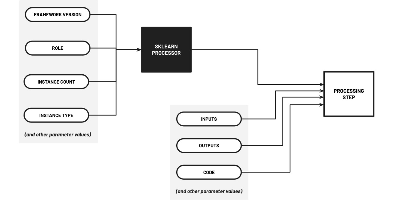
Figure 11.8 – Configuring and preparing the ProcessingStep

Here, we initialized the ProcessingStep object using the configured SKLearnProcessor object along with the parameter values for the inputs, outputs, and code parameters.

7. Next, let’s prepare the model_path variable to point to where the model will be uploaded after the SageMaker training job has finished (when the ML pipeline is executed during a later step):

   model_path = f"s3://{s3_bucket}/{prefix}/model/"
8. Additionally, let’s prepare the model_id variable to store the ID of the ML model we’ll use:

   model_id = "autogluon-classification-ensemble"
9. Let’s specify the region we are using inside region_name:

   region_name = "us-west-2"
10. Use image_uris.retrieve() to get the ECR container image URI of our training image:

    from sagemaker import image_uris
    train_image_uri = image_uris.retrieve(
        region=region_name,
        framework=None,
        model_id=model_id,
        model_version="*",
        image_scope="training",
        instance_type="ml.m5.xlarge",
    )

If you are wondering what the value of train_image_uri is, it should have a string value equal (or similar to): '763104351884.dkr.ecr.us-west-2.amazonaws.com/autogluon-training:0.4.0-cpu-py38'.

11. Use script_uris.retrieve() to get the script S3 URI associated with the model (given the values of model_id, model_version, and script_scope):

    from sagemaker import script_uris
    train_source_uri = script_uris.retrieve(
        model_id=model_id, 
        model_version="*", 
        script_scope="training"
    )

Note that train_source_uri should have a string value equal (or similar) to 's3://jumpstart-cache-prod-us-west-2/source-directory-tarballs/autogluon/transfer_learning/classification/v1.0.1/sourcedir.tar.gz'.

Note

What’s inside this sourcedir.tar.gz file? If the script_scope value used when calling script_uris.retrieve() is "training", the sourcedir.tar.gz file should contain code that uses autogluon.tabular.TabularPredictor when training the ML model. Note that the contents of sourcedir.tar.gz change depending on the arguments specified when calling script_uris.retrieve().

12. Use model_uris.retrieve() to get the model artifact S3 URI associated with the model (given the values of model_id, model_version, and model_scope):

    from sagemaker import model_uris
    train_model_uri = model_uris.retrieve(
        model_id=model_id, 
        model_version="*", 
        model_scope="training"
    )

Note that train_model_uri should have a string value equal (or similar) to 's3://jumpstart-cache-prod-us-west-2/autogluon-training/train-autogluon-classification-ensemble.tar.gz'.

13. With the values for train_image_uri, train_source_uri, train_model_uri, and model_path ready, we can now initialize the Estimator object:

    from sagemaker.estimator import Estimator
    estimator = Estimator(
        image_uri=train_image_uri,
        source_dir=train_source_uri,
        model_uri=train_model_uri,
        entry_point="transfer_learning.py",
        instance_count=1,
        instance_type="ml.m5.xlarge",
        max_run=900,
        output_path=model_path,
        session=session,
        role=role
    )

Here, the entry_point value points to the transfer_learning.py script file stored inside sourcedir.tar.gz containing the relevant scripts for training the model.

14. Next, let’s use the retrieve_default() function to retrieve the default set of hyperparameters for our AutoGluon classification model:

    from sagemaker.hyperparameters import retrieve_default
    hyperparameters = retrieve_default(
        model_id=model_id, 
        model_version="*"
    )
    hyperparameters["verbosity"] = "3"
    estimator.set_hyperparameters(**hyperparameters) 
15. Prepare the TrainingStep object that uses the Estimator object as one of the parameter values during initialization:

    s3_data = step_process         
        .properties                
        .ProcessingOutputConfig    
        .Outputs["split"]          
        .S3Output.S3Uri            
    step_train = TrainingStep(
        name="TrainModel",
        estimator=estimator,
        inputs={
            "training": TrainingInput(
                s3_data=s3_data,
            )
        },
    )

Here, s3_data contains a Properties object that points to the path where the output files of the SageMaker Processing job (from the previous step of the pipeline) will be stored when the ML pipeline runs. If we inspect s3_data using s3_data.__dict__, we should get a dictionary similar to the following:

{'step_name': 'PrepareData',
 'path':  "ProcessingOutputConfig.Outputs['split']
           .S3Output.S3Uri",
 '_shape_names': ['S3Uri'],
 '__str__': 'S3Uri'} 

To help us visualize how we configured the TrainingStep object, let’s quickly check Figure 11.9:

Figure 11.9 – Configuring and preparing the TrainingStep object

Here, we initialize the TrainingStep object using the configured Estimator object along with the parameter values for the name and inputs parameters.

16. Now, let’s use image_uris.retrieve() and script_uris.retrieve() to retrieve the container image URI and script URI for the deployment of AutoGluon classification models:

    deploy_image_uri = image_uris.retrieve(
        region=region_name,
        framework=None,
        image_scope="inference",
        model_id=model_id,
        model_version="*",
        instance_type="ml.m5.xlarge",
    )
    deploy_source_uri = script_uris.retrieve(
        model_id=model_id, 
        model_version="*", 
        script_scope="inference"
    )
17. Use the aws s3 cp command to download the sourcedir.tar.gz file to the tmp directory:

    !aws s3 cp {deploy_source_uri} tmp/sourcedir.tar.gz
18. Next, upload the sourcedir.tar.gz file from the tmp directory to your S3 bucket:

    updated_source_uri = f's3://{s3_bucket}/{prefix}' + 
                          '/sourcedir/sourcedir.tar.gz'
    !aws s3 cp tmp/sourcedir.tar.gz {updated_source_uri}
19. Let’s define the random_string() function:

    import uuid
    def random_string():
        return uuid.uuid4().hex.upper()[0:6]

This function should return a random alphanumeric string (with 6 characters).

20. With the values for deploy_image_uri, updated_source_uri, and model_data ready, we can now initialize the Model object:

    from sagemaker.model import Model
    from sagemaker.workflow.pipeline_context import 
        PipelineSession
    pipeline_session = PipelineSession()
    model_data = step_train    
        .properties            
        .ModelArtifacts        
        .S3ModelArtifacts      
    model = Model(image_uri=deploy_image_uri, 
                  source_dir=updated_source_uri,
                  model_data=model_data,
                  role=role,
                  entry_point="inference.py",
                  sagemaker_session=pipeline_session,
                  name=random_string())

Here, we use the random_string() function that we defined in the previous step for the name identifier of the Model object.

21. Next, let’s prepare the ModelStep object that uses the output of model.register() during initialization:

    from sagemaker.workflow.model_step import ModelStep
    model_package_group_name = "AutoGluonModelGroup"
    register_args = model.register(
        content_types=["text/csv"],
        response_types=["application/json"],
        inference_instances=["ml.m5.xlarge"],
        transform_instances=["ml.m5.xlarge"],
        model_package_group_name=model_package_group_name,
        approval_status="Approved",
    )
    step_model_create = ModelStep(
        name="CreateModel",
        step_args=register_args
    )
22. Now, let’s initialize the Pipeline object using the different step objects we prepared in the previous steps:

    pipeline_name = f"PARTIAL-PIPELINE"
    partial_pipeline = Pipeline(
        name=pipeline_name,
        parameters=[
            input_data
        ],
        steps=[
            step_process, 
            step_train,
            step_model_create,
        ],
    )
23. Finally, let’s use the upsert() method to create our ML pipeline:

    partial_pipeline.upsert(role_arn=role)

Note

Note that the upsert() method can be used to update an existing ML pipeline, too.

Now that our initial pipeline is ready, we can proceed with running the ML pipeline!

Running our first ML pipeline

Once the Pipeline object has been initialized and created, we can run it right away using the start() method, which is similar to what we have in the following line of code:

execution = partial_pipeline.start()

If we wish to override the default parameters of the pipeline inputs (for example, the input data used), we can specify parameter values when calling the start() method similar to what we have in the following block of code:

execution = partial_pipeline.start(
    parameters=dict(
        RawData="<INSERT NEW SOURCE PATH>",
    )
)

Once the pipeline execution starts, we can then use execution.wait() to wait for the pipeline to finish running.

With this in mind, let’s run our ML pipeline in the next set of steps:

1. With everything ready, let’s run the (partial) ML pipeline using the start() method:

   execution = partial_pipeline.start()
   execution.describe()
2. Let’s use the wait() method to wait for the pipeline to complete before proceeding:

   execution.wait()

Note

This should take around 10–15 minutes to complete. Feel free to grab a cup of coffee or tea while waiting!

3. Run the following block of code to get the resulting model package ARN:

   steps = execution.list_steps()
   steps[0]['Metadata']['RegisterModel']['Arn']

This should yield an ARN with a format similar to arn:aws:sagemaker:us-west-2:<ACCOUNT ID>:model-package/autogluonmodelgroup/1. Copy this value into your text editor. We will use this model package ARN later when testing our Lambda functions in the Creating Lambda functions for deployment section of this chapter.

4. Locate and click on the triangle icon (SageMaker resources) near the bottom of the left-hand sidebar of SageMaker Studio (as highlighted in Figure 11.10):

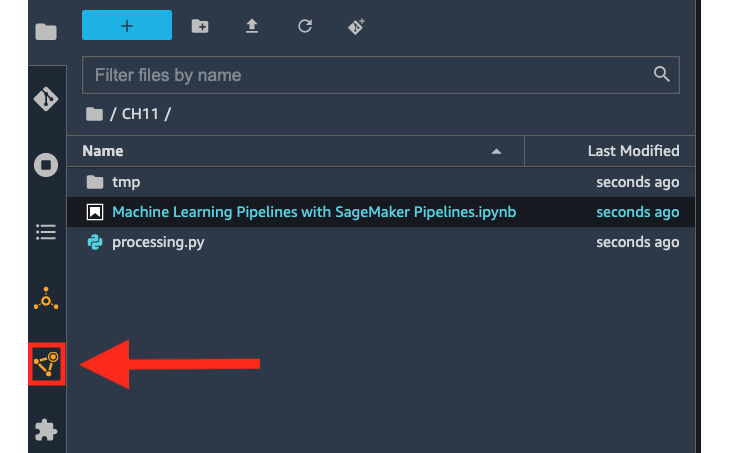
Figure 11.10 – Opening the SageMaker resources pane

This should open the SageMaker resources pane where we can view and inspect a variety of SageMaker resources.

5. Select Pipelines from the list of options available in the drop-down menu in the SageMaker resources pane.
6. After that, double-click on the row that maps to the PARTIAL-PIPELINE pipeline we just created. After that, double-click on the row that maps to the pipeline execution we triggered after calling partial_pipeline.start().
7. Once the execution has finished, you should see a graph that is similar to what is shown in Figure 11.11:

Figure 11.11 – Completed pipeline execution

Feel free to click on the rounded rectangles to check the following details of each of the steps:

• Input – The input files, parameters, and configuration
• Output – The output files and metrics (if any)
• Logs – The generated logs
• Information – Any additional information/metadata

8. Navigate back to the tab corresponding to the Machine Learning Pipelines with SageMaker Pipelines.ipynb notebook.
9. Let’s review the steps executed during the (partial) pipeline run using the list_steps() method:

   execution.list_steps()

This should return a list of dictionaries that map to the executed steps of the pipeline.

We are not yet done! At this point, we have only finished half of our ML pipeline. Make sure that you do not turn off the running apps and instances in SageMaker Studio, as we will be running more blocks of code inside the Machine Learning Pipelines with SageMaker Pipelines.ipynb notebook later to complete our pipeline.

Note

If you need to take a break, you may turn off the running instances and apps (to manage costs), and then run all the cells again in the Machine Learning Pipelines with SageMaker Pipelines.ipynb notebook before working on the Completing the end-to-end ML pipeline section of this chapter.

Creating Lambda functions for deployment

Our second (and more complete pipeline) will require a few additional resources to help us deploy our ML model. In this section, we will create the following Lambda functions:

• check-if-endpoint-exists – This is a Lambda function that accepts the name of the ML inference endpoint as input and returns True if the endpoint exists already.
• deploy-model-to-new-endpoint – This is a Lambda function that accepts the model package ARN as input (along with the role and the endpoint name) and deploys the model into a new inference endpoint
• deploy-model-to-existing-endpoint – This is a Lambda function that accepts the model package ARN as input (along with the role and the endpoint name) and deploys the model into an existing inference endpoint (by updating the deployed model inside the ML instance)

We will use these functions later in the Completing the end-to-end ML pipeline section to deploy the ML model we will register in the SageMaker Model Registry (using ModelStep).

Preparing the Lambda function for deploying a model to a new endpoint

The first AWS Lambda function we will create will be configured and programmed to deploy a model to a new endpoint. To help us visualize how our function will work, let’s quickly check Figure 11.12:

Figure 11.12 – Deploying a model to a new endpoint

This function will accept the following input parameters: an IAM role, the endpoint name, and the model package ARN. After receiving these input parameters, the function will create the corresponding set of resources needed to deploy the model (from the model package) to a new ML inference endpoint.

In the next set of steps, we will create a Lambda function that we will use to deploy an ML model to a new inference endpoint:

1. Navigate to the Lambda Management console by typing lambda in the search bar of the AWS Management Console, and then clicking on the Lambda link from the list of search results.

Note

In this chapter, we will create and manage our resources in the Oregon (us-west-2) region. Make sure that you have set the correct region before proceeding with the next steps.

2. Locate and click on the Create function button (located in the upper-left corner of the Functions page). In the Create function page, select Author from scratch when choosing an option to create our function. Additionally, specify the following configuration under Basic information:
   • Function name: deploy-model-to-new-endpoint
   • Runtime: Python 3.9
   • Permissions > Change default execution role
   • Execution role: Use an existing role
   • Existing role: pipeline-lambda-role
3. Scroll down to the bottom of the page and then click on the Create function button.

Note

You should see the following success notification after clicking on the Create function button: Successfully created the function deploy-model-to-new-endpoint. You can now change its code and configuration. To invoke your function with a test event, choose Test.

4. Navigate to the Configuration tab. Under General configuration, click on the Edit button. This should redirect you to the Edit basic settings page. Specify the following configuration values on the Edit basic settings page:
   • Memory: 1024 MB
   • Timeout: 15 min 0 sec

Afterward, click on the Save button.

5. Open the following link in another browser tab: https://raw.githubusercontent.com/PacktPublishing/Machine-Learning-Engineering-on-AWS/main/chapter11/utils.py. Copy the contents of the page into your clipboard using Ctrl + A and then Ctrl + C (or, alternatively, CMD + A and then CMD + C if you are using a Mac).
6. Back in the browser tab showing the Lambda console, navigate to the Code tab. Under Code source, open the File menu and then select New File. This will open a new tab named Untitled1.
7. In the new tab (containing no code), paste the code copied to the clipboard. Open the File menu and then select Save from the list of options. Specify utils.py as the Filename field value, and then click on Save.
8. Navigate to the tab where we can modify the code inside lambda_function.py. Delete the boilerplate code currently stored inside lambda_function.py before proceeding.

Note

Type (or copy) the code blocks in the succeeding set of steps inside lambda_function.py. You can find a copy of the code for the Lambda function at https://github.com/PacktPublishing/Machine-Learning-Engineering-on-AWS/blob/main/chapter11/deploy-model-to-new-endpoint.py.

9. In the lambda_function.py file, import the functions we will need for deploying a trained ML model to a new ML inference endpoint:

   import json
   from utils import (
       create_model, 
       create_endpoint_config, 
       create_endpoint, 
       random_string,
       block
   )
10. Now, let’s define the lambda_handler() function:

    def lambda_handler(event, context):
        role = event['role']
        endpoint_name = event['endpoint_name']
        package_arn = event['package_arn']
        
        model_name = 'model-' + random_string()
        
        with block('CREATE MODEL'):
            create_model(
                model_name=model_name,
                package_arn=package_arn,
                role=role
            )
        
        with block('CREATE ENDPOINT CONFIG'):
            endpoint_config_name = create_endpoint_config(
                model_name
            )
        
        with block('CREATE ENDPOINT'):
            create_endpoint(
                endpoint_name=endpoint_name, 
                endpoint_config_name=endpoint_config_name
            )
            
        return {
            'statusCode': 200,
            'body': json.dumps(event),
            'model': model_name
        }
11. Click on the Deploy button.
12. Click on the Test button.
13. In the Configure test event pop-up window, specify test under Event name, and then specify the following JSON value under Event JSON:

    {
      "role": "<INSERT SAGEMAKER EXECUTION ROLE ARN>",
      "endpoint_name": "AutoGluonEndpoint",
      "package_arn": "<INSERT MODEL PACKAGE ARN>"
    }

Make sure that you replace the following values:

• <INSERT SAGEMAKER EXECUTION ROLE ARN> – Replace this placeholder value with the Execution Role ARN copied to your text editor in the Preparing the essential prerequisites section of this chapter. The Execution Role ARN should follow a format similar to arn:aws:iam::1234567890:role/service-role/AmazonSageMaker-ExecutionRole-20220000T000000.
• <INSERT MODEL PACKAGE ARN> – Replace this placeholder value with the model package ARN copied to your text editor in the Running our first pipeline with SageMaker Pipelines section of this chapter. The model package ARN should follow a format similar to arn:aws:sagemaker:us-west-2:1234567890:model-package/autogluonmodelgroup/1.

14. Copy this test event JSON value to the text editor on your local machine. We will use this test event JSON again later when testing our deploy-model-to-existing-endpoint Lambda function.
15. Afterward, click on the Save button.
16. With everything ready, let’s click on the Test button. This should open a new tab that should show the execution results after a few minutes.

Note

This step might take 5–15 minutes to complete. Feel free to grab a cup of coffee or tea!

17. While waiting, scroll up and locate the Function overview pane. Copy the Function ARN value to your text editor. We will use this Function ARN value later in the Completing the end-to-end ML pipeline section of this chapter.

Once the deploy-model-to-new-endpoint Lambda function has finished running, we should have our ML model deployed already in an ML inference endpoint. Note that we are just testing the Lambda function, and we will delete the ML inference endpoint (launched by the deploy-model-to-new-endpoint Lambda function) in a later step before running the complete ML pipeline.

Preparing the Lambda function for checking whether an endpoint exists

The second AWS Lambda function we will create will be configured and programmed to check whether an endpoint exists already (given the endpoint name). To help us visualize how our function will work, let’s quickly check Figure 11.13:

Figure 11.13 – Check whether an endpoint exists already

This function will accept one input parameter—the name of the ML inference endpoint. After receiving the input parameter, the function will use the boto3 library to list all running endpoints in the region and check whether the name of one of these endpoints matches the input parameter value.

In the next set of steps, we will create a Lambda function that we will use to check whether an ML inference endpoint exists already:

1. Open a new browser tab and navigate to the Functions page of the Lambda Management console.
2. Locate and click on the Create function button (located in the upper-left corner of the Functions page), and then specify the following configuration values:
   • Author from scratch
   • Function name: check-if-endpoint-exists
   • Runtime: Python 3.9
   • Permissions > Change default execution role
   • Execution role: Use an existing role
   • Existing role: pipeline-lambda-role
3. Scroll down to the bottom of the page, and then click on the Create function button.

Note

Type (or copy) the code blocks into the succeeding set of steps inside lambda_function.py. You can find a copy of the code for the Lambda function here at https://github.com/PacktPublishing/Machine-Learning-Engineering-on-AWS/blob/main/chapter11/check-if-endpoint-exists.py.

4. In the lambda_function.py file, import boto3 and initialize the client for the SageMaker service:

   import boto3
   sm_client = boto3.client('sagemaker')
5. Next, let’s define the endpoint_exists() function:

   def endpoint_exists(endpoint_name):
       response = sm_client.list_endpoints(
           NameContains=endpoint_name
       )
       
       results = list(
           filter(
               lambda x: 
               x['EndpointName'] == endpoint_name, 
               
               response['Endpoints']
           )
       )
       
       return len(results) > 0
6. Now, let’s define the lambda_handler() function that makes use of the endpoint_exists() function to check whether an ML inference endpoint exists or not (given the endpoint name):

   def lambda_handler(event, context):
       endpoint_name = event['endpoint_name']
       
       return {
           'endpoint_exists': endpoint_exists(
               endpoint_name=endpoint_name
           )
       }
7. Click on the Deploy button.
8. Click on the Test button. In the Configure test event pop-up window, specify test under Event name and then specify the following JSON value under Event JSON:

   {
     "endpoint_name": "AutoGluonEndpoint"
   }
9. Afterward, click on the Save button.
10. With everything ready, let’s click on the Test button. This should open a new tab that will show the execution results after a few seconds. We should get the following response value after testing the Lambda function:

    {
      "endpoint_exists": true
    }
11. Finally, scroll up and locate the Function overview pane. Copy the Function ARN value to your text editor. We will use this Function ARN value later in the Completing the end-to-end ML pipeline section of this chapter.

Now that we have finished preparing and testing the check-if-endpoint-exists Lambda function, we can proceed with creating the last Lambda function (deploy-model-to-existing-endpoint).

Preparing the Lambda function for deploying a model to an existing endpoint

The third AWS Lambda function we will create will be configured and programmed to deploy a model to an existing endpoint. To help us visualize how our function will work, let’s quickly check Figure 11.14:

Figure 11.14 – Deploying a model to an existing endpoint

This function will accept three input parameters—an IAM role, the endpoint name, and the model package ARN. After receiving these input parameters, the function will perform the necessary steps to update the model deployed in an existing ML inference endpoint with the model from the model package provided.

In the next set of steps, we will create a Lambda function that we will use to deploy an ML model to an existing inference endpoint:

1. Open a new browser tab and navigate to the Functions page of the Lambda Management console.
2. Locate and click on the Create function button (located in the upper-left corner of the Functions page), and then specify the following configuration values:
   • Author from scratch
   • Function name: deploy-model-to-existing-endpoint
   • Runtime: Python 3.9
   • Permissions > Change default execution role
   • Execution role: Use an existing role
   • Existing role: pipeline-lambda-role
3. Scroll down to the bottom of the page and then click on the Create function button.
4. Navigate to the Configuration tab. Under General configuration, click on the Edit button. This should redirect you to the Edit basic settings page. Specify the following configuration values in the Edit basic settings page:
   • Memory: 1024 MB
   • Timeout: 15 min 0 sec
5. Afterward, click on the Save button.
6. Open the following link in another browser tab: https://raw.githubusercontent.com/PacktPublishing/Machine-Learning-Engineering-on-AWS/main/chapter11/utils.py. Copy the contents of the page into your clipboard using Ctrl + A and then Ctrl + C (or, alternatively, CMD + A and then CMD + C if you are using a Mac).
7. Back in the browser tab showing the Lambda console, navigate to the Code tab. Under Code source, open the File menu and then select New File. This will open a new tab named Untitled1. In the new tab (containing no code), paste the code copied to the clipboard.
8. Open the File menu and then select Save from the list of options. Specify utils.py as the Filename field value and then click on Save.
9. Navigate to the tab where we can modify the code inside lambda_function.py. Delete the boilerplate code currently stored inside lambda_function.py before proceeding.

Note

Type (or copy) the code blocks in the succeeding set of steps inside lambda_function.py. You can find a copy of the code for the Lambda function at https://github.com/PacktPublishing/Machine-Learning-Engineering-on-AWS/blob/main/chapter11/deploy-model-to-existing-endpoint.py.

10. In the lambda_function.py file, import the functions we will need to update the deployed model of an existing endpoint:

    import json
    from utils import (
        create_model, 
        create_endpoint_config, 
        update_endpoint, 
        random_string,
        block
    )
11. Now, let’s define the lambda_handler() function using the following block of code:

    def lambda_handler(event, context):
        role = event['role']
        endpoint_name = event['endpoint_name']
        package_arn = event['package_arn']
        
        model_name = 'model-' + random_string()
        
        with block('CREATE MODEL'):
            create_model(
                model_name=model_name,
                package_arn=package_arn,
                role=role
            )
        
        with block('CREATE ENDPOINT CONFIG'):
            endpoint_config_name = create_endpoint_config(
                model_name
            )
        
        with block('UPDATE ENDPOINT'):
            update_endpoint(
                endpoint_name=endpoint_name, 
                endpoint_config_name=endpoint_config_name
            )
            
        return {
            'statusCode': 200,
            'body': json.dumps(event),
            'model': model_name
        } 
12. Click on the Deploy button.
13. Click on the Test button. In the Configure test event pop-up window, specify test under Event name and then specify the following JSON value under Event JSON:

    {
      "role": "<INSERT SAGEMAKER EXECUTION ROLE ARN>",
      "endpoint_name": "AutoGluonEndpoint",
      "package_arn": "<INSERT MODEL PACKAGE ARN>"
    }

Make sure that you replace the following values:

• <INSERT SAGEMAKER EXECUTION ROLE ARN> – Replace this placeholder value with the Execution Role ARN copied to your text editor in the Preparing the essential prerequisites section of this chapter.
• <INSERT MODEL PACKAGE ARN> – Replace this placeholder value with the model package ARN copied to your text editor in the Running our first pipeline with SageMaker Pipelines section of this chapter.

Additionally, you can use the same test event JSON value that we copied to our text editor while testing our deploy-model-to-new-endpoint Lambda function.

14. Afterward, click on the Save button.
15. With everything ready, let’s click on the Test button. This should open a new tab that should show the execution results after a few minutes.

Note

This step may take 5–15 minutes to complete. Feel free to grab a cup of coffee or tea!

16. While waiting, scroll up and locate the Function overview pane. Copy the Function ARN value to your text editor. We will use this Function ARN value later in the Completing the end-to-end ML pipeline section of this chapter.

With all the Lambda functions ready, we can now proceed with testing our ML inference endpoint (before completing the end-to-end ML pipeline).

Note

At this point, we should have 3 x Function ARN values in our text editor. This includes the ARNs for the check-if-endpoint-exists Lambda function, the deploy-model-to-new-endpoint Lambda function, and the deploy-model-to-existing-endpoint Lambda function. We will use these ARN values later in the Completing the end-to-end ML pipeline section of this chapter.

Testing our ML inference endpoint

Of course, we need to check whether the ML inference endpoint is working! In the next set of steps, we will download and run a Jupyter notebook (named Test Endpoint and then Delete.ipynb) that tests our ML inference endpoint using the test dataset:

1. Let’s begin by opening the following link in another browser tab: https://bit.ly/3xyVAXz
2. Right-click on any part of the page to open a context menu, and then choose Save as... from the list of available options. Save the file as Test Endpoint then Delete.ipynb, and then download it to the Downloads folder (or similar) on your local machine.
3. Navigate back to your SageMaker Studio environment. In the File Tree (located on the left-hand side of the SageMaker Studio environment), make sure that you are in the CH11 folder similar to what we have in Figure 11.15:

Figure 11.15 – Uploading the test endpoint and then the Delete.ipynb file

4. Click on the upload button (as highlighted in Figure 11.15), and then select the Test Endpoint then Delete.ipynb file that we downloaded in an earlier step.

Note

This should upload the Test Endpoint then Delete.ipynb notebook file from your local machine to the SageMaker Studio environment (in the CH11 folder).

5. Double-click on the Test Endpoint then Delete.ipynb file in the File tree to open the notebook in the Main work area (which contains tabs of the open notebooks, files, and terminals).
6. Update the first cell with the name of the S3 bucket used in the Machine Learning Pipelines with SageMaker Pipelines.ipynb notebook:

   s3_bucket = '<INSERT S3 BUCKET HERE>'

Make sure to replace <INSERT S3 BUCKET HERE> with the S3 bucket name we copied to our text editor earlier in the Preparing the essential prerequisites section of this chapter.

7. Open the Run menu and select Run All Cells to execute all the blocks of code in the Test Endpoint then Delete.ipynb notebook.

Note

It should take around 1–2 minutes to run all the cells in the Jupyter notebook. Feel free to grab a cup of coffee or tea while waiting!

8. Once all the cells in the Test Endpoint then Delete.ipynb notebook have been executed, locate the cell containing the following block of code (along with the returned output):

   from sklearn.metrics import accuracy_score
   accuracy_score(actual_list, predicted_list)

Verify that the model got an accuracy score equal to or close to 0.88 (or 88%).

At this point, the ML inference endpoint should be in a deleted state since the Test Endpoint then Delete.ipynb Jupyter notebook also runs the predictor.delete_endpoint() line after computing for the ML model metrics.

Completing the end-to-end ML pipeline

In this section, we will build on top of the (partial) pipeline we prepared in the Running our first pipeline with SageMaker Pipelines section of this chapter. In addition to the steps and resources used to build our partial pipeline, we will also utilize the Lambda functions we created (in the Creating Lambda functions for deployment section) to complete our ML pipeline.

Defining and preparing the complete ML pipeline

The second pipeline we will prepare would be slightly longer than the first pipeline. To help us visualize how our second ML pipeline using SageMaker Pipelines will look like, let’s quickly check Figure 11.16:

Figure 11.16 – Our second ML pipeline using SageMaker Pipelines

Here, we can see that our pipeline accepts two input parameters—the input dataset and the endpoint name. When the pipeline runs, the input dataset is first split into training, validation, and test sets. The training and validation sets are then used to train an ML model, which then gets registered to the SageMaker Model Registry. After that, the pipeline checks whether an ML inference endpoint with the provided endpoint name exists already. If the endpoint does not exist yet, the model is deployed to a new endpoint. Otherwise, the model of an existing endpoint (with the provided endpoint name) is updated using the model trained during the pipeline execution.

In the next set of steps, we will create a new ML pipeline using the steps and resources configured in the Machine Learning Pipelines with SageMaker Pipelines.ipynb notebook:

1. Navigate back to the tab corresponding to the Machine Learning Pipelines with SageMaker Pipelines.ipynb notebook.

Note

We will run the blocks of code in the succeeding set of steps inside the Machine Learning Pipelines with SageMaker Pipelines.ipynb notebook (after the existing set of cells). If you turned off the kernel and/or the SageMaker Studio instance after running the commands in the Running our first pipeline with SageMaker Pipelines section, make sure that you run all the cells again (and wait for the pipeline to finish running) by selecting Run All Cells from the list of options under the Run menu.

2. Let’s initialize the ParameterString object that maps to the Pipeline parameter for the name of the ML inference endpoint (which will be created or updated after the ML pipeline has finished running):

   input_endpoint_name = ParameterString(
       name="EndpointName",
       default_value=f'AutoGluonEndpoint', 
   )
3. Next, let’s import the classes we will need to complete the end-to-end ML pipeline:

   from sagemaker.workflow.lambda_step import (
       LambdaStep, 
       LambdaOutput, 
       LambdaOutputTypeEnum
   )
   from sagemaker.lambda_helper import (
       Lambda
   )
   from sagemaker.workflow.conditions import (
       ConditionEquals
   )
   from sagemaker.workflow.condition_step import (
       ConditionStep, 
       JsonGet
   )
4. Prepare the LambdaOutput object that will map (later) to the output of a LambdaStep object:

   output_endpoint_exists = LambdaOutput(
       output_name="endpoint_exists", 
       output_type=LambdaOutputTypeEnum.Boolean
   )
5. Initialize the LambdaStep object, which maps to the Lambda function that checks whether a specified ML inference endpoint exists already (given the endpoint name):

   package_arn = step_model_create 
       .properties.ModelPackageArn
   endpoint_exists_lambda = LambdaStep(
       name="CheckIfEndpointExists",
       lambda_func=Lambda(
           function_arn="<INSERT FUNCTION ARN>"
       ),
       inputs={
           "endpoint_name": input_endpoint_name,
           "package_arn": package_arn
       },
       outputs=[output_endpoint_exists]
   )

Make sure to replace <INSERT FUNCTION ARN> with the ARN of the check-if-endpoint-exists Lambda function we copied into our text editor. It should have a format that is similar to arn:aws:lambda:us-west-2:<ACCOUNT ID>:function:check-if-endpoint-exists.

6. Next, initialize the LambdaStep object, which maps to the Lambda function that deploys the trained ML model to an existing ML inference endpoint:

   step_lambda_deploy_to_existing_endpoint = LambdaStep(
       name="DeployToExistingEndpoint",
       lambda_func=Lambda(
           function_arn="<INSERT FUNCTION ARN>"
       ),
       inputs={
           "role": role,
           "endpoint_name": input_endpoint_name,
           "package_arn": package_arn
       },
       outputs=[]
   )

Make sure that you replace <INSERT FUNCTION ARN> with the ARN of the deploy-model-to-existing-endpoint Lambda function we copied into our text editor. It should have a format similar to arn:aws:lambda:us-west-2:<ACCOUNT ID>:function: deploy-model-to-existing-endpoint.

7. After that, initialize the LambdaStep object, which maps to the Lambda function that deploys the trained ML model to a new ML inference endpoint:

   step_lambda_deploy_to_new_endpoint = LambdaStep(
       name="DeployToNewEndpoint",
       lambda_func=Lambda(
           function_arn="<INSERT FUNCTION ARN>"
       ),
       inputs={
           "role": role,
           "endpoint_name": input_endpoint_name,
           "package_arn": package_arn
       },
       outputs=[]
   )

Make sure that you replace <INSERT FUNCTION ARN> with the ARN of the deploy-model-to-new-endpoint Lambda function we copied into our text editor. It should have a format that is similar to arn:aws:lambda:us-west-2:<ACCOUNT ID>:function: deploy-model-to-new-endpoint.

8. With the three LambdaStep objects ready, let’s prepare the ConditionStep object, which checks whether an endpoint exists already (using the output of the endpoint_exists_lambda LambdaStep object):

   left = endpoint_exists_lambda 
       .properties               
       .Outputs['endpoint_exists']
   cond_equals = ConditionEquals(
       left=left,
       right=True
   )
   if_steps = [step_lambda_deploy_to_existing_endpoint]
   else_steps = [step_lambda_deploy_to_new_endpoint]
   step_endpoint_exists_condition = ConditionStep(
       name="EndpointExists",
       conditions=[cond_equals],
       if_steps=if_steps,
       else_steps=else_steps
   )

This step tells the ML pipeline to do the following:

• Deploy the model to a new endpoint if the endpoint does not exist yet.
• Deploy the model to an existing endpoint if the endpoint exists already.

To help us visualize how we configured the ConditionStep object, let’s quickly check Figure 11.17:

Figure 11.17 – Configuring and preparing the ConditionStep object

Here, we can see that the ConditionStep object is initialized with several parameters—conditions, if_steps, and else_steps (in addition to name of the endpoint). If EndpointExists LambdaStep returns True, then DeployToExistingEndpoint LambdaStep is executed. Otherwise, DeployToNewEndpoint LambdaStep is executed instead.

9. With all of the steps ready, let’s initialize a new Pipeline object using the different step objects we prepared:

   pipeline_name = f"COMPLETE-PIPELINE"
   complete_pipeline = Pipeline(
       name=pipeline_name,
       parameters=[
           input_data,
           input_endpoint_name
       ],
       steps=[
           step_process, 
           step_train,
           step_model_create,
           endpoint_exists_lambda, 
           step_endpoint_exists_condition
       ],
   )
   complete_pipeline.upsert(role_arn=role)

Note that this pipeline is different and separate from the (partial) pipeline we prepared in the Running our first pipeline with SageMaker Pipelines section of this chapter. We should see that this pipeline has a few more additional steps once we run it in the next section.

Running the complete ML pipeline

With everything ready, we can now run our end-to-end ML pipeline. Compared to the (partial) pipeline we executed in the Running our first pipeline with SageMaker Pipelines section of this chapter, our (complete) pipeline allows us to specify an optional name of the ML inference endpoint (Note: Do not run the following block of code):

execution = complete_pipeline.start(
    parameters=dict(
        EndpointName="<INSERT NEW ENDPOINT NAME>",
    )
)

If the endpoint name is not specified, the pipeline proceeds with using the default endpoint name value (that is, AutoGluonEndpoint) during pipeline execution.

In the next set of steps, we will run our pipeline, wait for it to deploy a trained ML model to a new inference endpoint, and then test the deployed model using the test dataset:

1. Continuing where we left off after running the last block of code in the Machine Learning Pipelines with SageMaker Pipelines.ipynb notebook, let’s run the end-to-end ML pipeline using the following block of code:

   execution = complete_pipeline.start()
   execution.describe()
2. Next, let’s use the wait() method to wait for the entire pipeline to complete:

   execution.wait()

Note

The pipeline execution should take around 15–30 minutes to complete. Feel free to grab a cup of coffee or tea while waiting!

3. While waiting, locate and click on the triangle icon (SageMaker resources) near the bottom of the left-hand sidebar of SageMaker Studio. This should open the SageMaker resources pane where we can view and inspect a variety of SageMaker resources.
4. Select Pipelines from the list of options available in the drop-down menu of the SageMaker resources pane.
5. After that, double-click on the row that maps to the COMPLETE-PIPELINE pipeline we just created. After that double-click on the row that maps to the pipeline execution we triggered. You should see a graph similar to what is shown in Figure 11.18:

Figure 11.18 – The ML pipeline is currently running the TrainModel step

Here, we can see that the PrepareData step has just been completed, and the ML pipeline is currently running the TrainModel step. As you can see, the COMPLETE-PIPELINE pipeline has more steps compared to the PARTIAL-PIPELINE pipeline we executed in the Running our first pipeline with SageMaker Pipelines section of this chapter.

6. After a few minutes, the graph should have more steps completed similar to what we have in Figure 11.19:

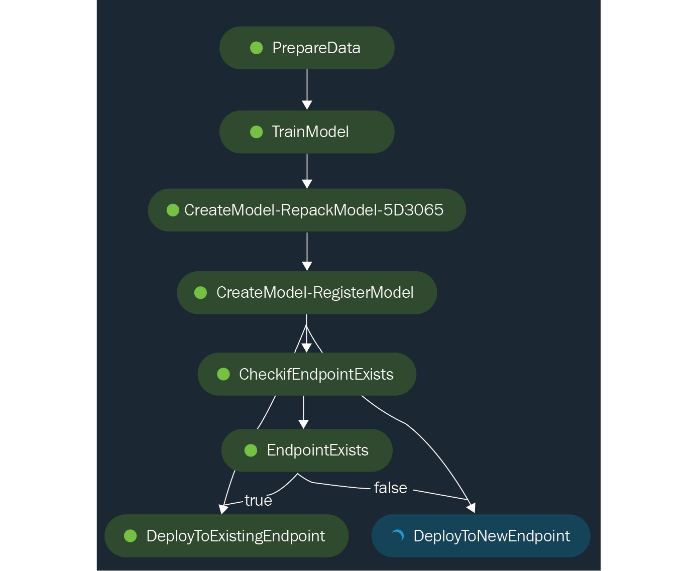
Figure 11.19 – The ML pipeline proceeds with running the DeployToNewEndpoint step

Here, we can see that since the ML endpoint does not exist yet (since we deleted it earlier while running the Test Endpoint then Delete.ipynb notebook), the ML pipeline proceeded with running the DeployToNewEndpoint step. Note that for succeeding runs, if the ML endpoint exists already, the DeployToExistingEndpoint step should run instead.

Important Note

Make sure that the execution role (attached to the SageMaker Domain) has the AWSLambda_FullAccess permission policy attached if you encounter the following error while running the Lambda functions: ClientError: User: <ARN> is not authorized to perform: lambda:InvokeFunction on resource: <arn> because no identity-based policy allows the lambda:InvokeFunction action. Feel free to check the Preparing the essential prerequisites section of this chapter for step-by-step instructions on how to update the permissions of the execution role.

7. Wait for the pipeline execution to finish. Once the pipeline has finished running, our AutoGluon model should be deployed inside an ML inference endpoint (named AutoGluonEndpoint).
8. Navigate back to the tab corresponding to the Test Endpoint then Delete.ipynb notebook. Open the Run menu, and then select Run All Cells to execute all the blocks of code in our Test Endpoint then Delete.ipynb notebook. Note that running all the cells in the notebook would also delete the existing ML inference endpoint (named AutoGluonEndpoint) after all cells have finished running.

Note

It should take 1–2 minutes to run all the cells in the Jupyter notebook. Feel free to grab a cup of coffee or tea while waiting!

9. Once all the cells in the Test Endpoint then Delete.ipynb notebook have been executed, locate the cell containing the following block of code (along with the output returned):

   from sklearn.metrics import accuracy_score
   accuracy_score(actual_list, predicted_list)

Verify that our model obtained an accuracy score equal to or close to 0.88 (or 88%). Note that this should be similar to what we obtained earlier in the Testing our ML inference endpoint section of this chapter.

What can we do with this pipeline? With this pipeline, by specifying different endpoint names for each pipeline run, we would be able to train and deploy a model to multiple endpoints. This should help us handle scenarios where we would need to manage dedicated ML inference endpoints for different environments (such as the production and staging environments). For example, we can have two running ML inference endpoints at the same time—AutoGluonEndpoint-production and AutoGluonEndpoint-staging. If we wish to generate a new model from a new dataset, we can trigger a pipeline run and specify the endpoint name for the staging environment instead of the production environment. This will help us test and verify the quality of the new model deployed in the staging environment and ensure that the production environment is always in a stable state. Once we need to update the production environment, we can simply trigger another pipeline run and specify the endpoint name associated with the production environment when training and deploying the new model.

Note

There are several ways to manage these types of deployments, and this is one of the options available for ML engineers and data scientists.

That’s pretty much it! Congratulations on being able to complete a relatively more complex ML pipeline! We were able to accomplish a lot in this chapter, and we should be ready to design and build our own custom pipelines.

Cleaning up

Now that we have completed working on the hands-on solutions of this chapter, it is time we clean up and turn off the resources we will no longer use. In the next set of steps, we will locate and turn off any remaining running instances in SageMaker Studio:

1. Make sure to check and delete all running inference endpoints under SageMaker resources (if any). To check whether there are running inference endpoints, click on the SageMaker resources icon and then select Endpoints from the list of options in the drop-down menu.
2. Open the File menu and select Shut down from the list of available options. This should turn off all running instances inside SageMaker Studio.

It is important to note that this cleanup operation needs to be performed after using SageMaker Studio. These resources are not turned off automatically by SageMaker even during periods of inactivity. Make sure to review whether all delete operations have succeeded before proceeding to the next section.

Note

Feel free to clean up and delete all the other resources in the AWS account (for example, the Cloud9 environment and the VPCs and Lambda functions we created), too.

Recommended strategies and best practices

Before we end this chapter (and this book), let’s quickly discuss some of the recommended strategies and best practices when using SageMaker Pipelines to prepare automated ML workflows. What improvements can we make to the initial version of our pipeline? Here are some of the possible upgrades we can implement to make our setup more scalable, more secure, and more capable of handling different types of ML and ML engineering requirements:

• Configure and set up autoscaling (automatic scaling) of the ML inference endpoint upon creation to dynamically adjust the number of resources used to handle the incoming traffic (of ML inference requests).
• Allow ML models to also be deployed in serverless and asynchronous endpoints (depending on the value of an additional pipeline input parameter) to help provide additional model deployment options for a variety of use cases.
• Add an additional step (or steps) in the pipeline that automatically evaluates the trained ML model using the test set and rejects the deployment of the model if the target metric value falls below a specified threshold score.
• Add an additional step in the pipeline that uses SageMaker Clarify to check for biases and drifts.
• Trigger a pipeline execution once an event happens through Amazon EventBridge (such as a file being uploaded in an Amazon S3 bucket).
• Cache specific pipeline steps to speed up repeated pipeline executions.
• Utilize Retry policies to automatically retry specific pipeline steps when exceptions and errors occur during pipeline executions.
• Use SageMaker Pipelines with SageMaker Projects for building complete ML workflows, which may involve CI/CD capabilities (using AWS services such as AWS CodeCommit and AWS CodePipeline).
• Update the IAM roles used in this chapter with a more restrictive set of permissions to improve the security of the setup.
• To manage the long-term costs of running SageMaker resources, we can utilize the Machine Learning Savings Plans, which involves reducing the overall cost of running resources after making a long-term commitment (for example, a 1-year or 3-year commitment)

There’s more we can add to this list, but these should do for now! Make sure that you review and check the recommended solutions and strategies shared in Chapter 9, Security, Governance, and Compliance Strategies, too.

Summary

In this chapter, we used SageMaker Pipelines to build end-to-end automated ML pipelines. We started by preparing a relatively simple pipeline with three steps—including the data preparation step, the model training step, and the model registration step. After preparing and defining the pipeline, we proceeded with triggering a pipeline execution that registered a newly trained model to the SageMaker Model Registry after the pipeline execution finished running.

Then, we prepared three AWS Lambda functions that would be used for the model deployment steps of the second ML pipeline. After preparing the Lambda functions, we proceeded with completing the end-to-end ML pipeline by adding a few additional steps to deploy the model to a new or existing ML inference endpoint. Finally, we discussed relevant best practices and strategies to secure, scale, and manage ML pipelines using the technology stack we used in this chapter.

You’ve finally reached the end of this book! Congratulations on completing all the chapters including the hands-on examples and solutions discussed in this book. It has been an amazing journey from start to finish, and it would be great if you can share this journey with others, too.

Further reading

At this point, you might want to dive deeper into the relevant subtopics discussed by checking the references listed in the Further reading section of each of the previous chapters. In addition to these, you can check the following resources, too:

• Amazon SageMaker Model Building Pipelines – Pipeline Steps (https://docs.aws.amazon.com/sagemaker/latest/dg/build-and-manage-steps.html)
• Boto3 – SageMaker Client (https://boto3.amazonaws.com/v1/documentation/api/latest/reference/services/sagemaker.html)
• Amazon SageMaker – AutoGluon-Tabular Algorithm (https://docs.aws.amazon.com/sagemaker/latest/dg/autogluon-tabular.html)
• Automate MLOps with SageMaker Projects (https://docs.aws.amazon.com/sagemaker/latest/dg/sagemaker-projects.html)
• Machine Learning Savings Plans (https://aws.amazon.com/savingsplans/ml-pricing/)
• SageMaker – Amazon EventBridge Integration (https://docs.aws.amazon.com/sagemaker/latest/dg/pipeline-eventbridge.html)