2

Deep Learning AMIs

In the Essential prerequisites section of Chapter 1, Introduction to ML Engineering on AWS, it probably took us about an hour or so to set up our Cloud9 environment. We had to spend a bit of time installing several packages, along with a few dependencies, before we were able to work on the actual machine learning (ML) requirements. On top of this, we had to make sure that we were using the right versions for certain packages to avoid running into a variety of issues. If you think this is error-prone and tedious, imagine being given the assignment of preparing 20 ML environments for a team of data scientists! Let me repeat that… TWENTY! It would have taken us around 15 to 20 hours of doing the same thing over and over again. After a week of using the ML environments you prepared, the data scientists then requested that you also install the deep learning frameworks TensorFlow, PyTorch, and MXNet inside these environments since they’ll be testing different deep learning models using these ML frameworks. At this point, you may already be asking yourself, “Is there a better way to do this?“. The good news is that there are a variety of ways to handle these types of requirements in a more efficient manner. One of the possible solutions is to utilize Amazon Machine Images (AMIs), specifically the AWS Deep Learning AMIs (DLAMIs) to significantly speed up the process of preparing ML environments. When launching new instances, these AMIs would serve as pre-configured templates containing the relevant software and environment configuration.

Before the DLAMIs existed, ML engineers had to spend hours installing and configuring deep learning frameworks inside EC2 instances before they could run ML workloads in the AWS cloud. The process of manually preparing these ML environments from scratch is tedious and error-prone as well. Once the DLAMIs were made available, data scientists and ML engineers were able to run their ML experiments straight away using their preferred deep learning framework.

In this chapter, we will see how convenient it is to set up a GPU instance using a framework-specific Deep Learning AMI. We will then train a deep learning model using TensorFlow and Keras inside this environment. Once the training step is complete, we will evaluate the model using a test dataset. After that, we will perform the cleanup steps and terminate the EC2 instance. Toward the end of this chapter, we will also have a short discussion on how AWS pricing works for EC2 instances. This will help equip you with the knowledge required to manage the overall cost of running ML workloads inside these instances.

That said, we will cover the following topics in this chapter:

• Getting started with Deep Learning AMIs
• Launching an EC2 instance using a Deep Learning AMI
• Downloading the sample dataset
• Training an ML model
• Loading and evaluating the model
• Cleaning up
• Understanding how AWS pricing works for EC2 instances

The hands-on solutions in this chapter will help you migrate any of your existing TensorFlow, PyTorch, and MXNet scripts and models to the AWS cloud. In addition to the cost discussions mentioned earlier, we will also talk about a few security guidelines and best practices to help us ensure that the environments we set up have a good starting security configuration. With these in mind, let’s get started!

Technical requirements

Before we start, we must have a web browser (preferably Chrome or Firefox) and an AWS account to use for the hands-on solutions in this chapter. Make sure that you have access to the AWS account you used in Chapter 1, Introduction to ML Engineering on AWS.

The Jupyter notebooks, source code, and other files used for each chapter are available in this book’s GitHub repository: https://github.com/PacktPublishing/Machine-Learning-Engineering-on-AWS.

Getting started with Deep Learning AMIs

Before we talk about DLAMIs, we must have a good idea of what AMIs are. We can think of an AMI as the “DNA” of an organism. Using this analogy, the organism would correspond and map to one or more EC2 instances:

Figure 2.1 – Launching EC2 instances using Deep Learning AMIs

If we were to launch two EC2 instances using the same AMI (similar to what is shown in Figure 2.1), both instances would have the same set of installed packages, frameworks, tools, and operating systems upon instance launch. Of course, not everything needs to be the same as these instances may have different instance types, different security groups, and other configurable properties.

AMIs allow engineers to easily launch EC2 instances in consistent environments without having to spend hours installing different packages and tools. In addition to the installation steps, these EC2 instances need to be configured and optimized before they can be used for specific workloads. Pre-built AMIs such as DLAMIs have popular deep learning frameworks such as TensorFlow, PyTorch, and MXNet pre-installed already. This means that data scientists, developers, and ML engineers may proceed with performing ML experiments and deployments without having to worry about the installation and setup process.

If we had to prepare 20 ML environments with these deep learning frameworks installed, I’m pretty sure that it would not take us 20 or more hours to do so. If we were to use DLAMIs, probably 2 to 3 hours would be more than enough to get the job done. You don’t believe me? In the next section, we will do just that! Of course, we will only be preparing a single ML environment instead of 20. While working on the hands-on solutions in this chapter, you will notice a significant speed boost when setting up and configuring the prerequisites needed to run the ML experiments.

Note

It is important to note that we have the option to build on top of existing AMIs and prepare our own custom AMIs. Then, we can use these custom AMIs when launching new EC2 instances.

Launching an EC2 instance using a Deep Learning AMI

Launching an EC2 instance from a DLAMI is straightforward. Once we have an idea of which DLAMI to use, the rest of the steps would just be focused on configuring and launching the EC2 instance. The cool thing here is that we are not limited to launching a single instance from an existing image. During the configuration stage, before an instance is launched from an AMI, it is important to note that we can specify the desired value for the number of instances to be launched (for example, 20). This would mean that instead of launching a single instance, we would launch 20 instances all at the same time instead.

Figure 2.2 – Steps to launch an EC2 instance using a DLAMI

We will divide this section into four parts. As shown in the preceding diagram, we’ll start by locating the framework-specific Deep Learning AMI in the AMI Catalog – a repository that contains a variety of AMIs that can be used when launching EC2 instances. We will then launch and configure an EC2 instance using the selected DLAMI and choose a GPU instance type, p3.2xlarge, as the instance type. We’ll then configure the security settings, including the network security settings, to be used by the instance. Finally, we will launch the instance and connect to it from the browser using EC2 Instance Connect.

Locating the framework-specific DLAMI

When looking for an AMI, the first place we should check is the AWS AMI Catalog. In the AMI Catalog, we should find a variety of DLAMIs. These DLAMIs can be categorized into either multi-framework DLAMIs or framework-specific DLAMIs. What’s the difference? Multi-framework DLAMIs include multiple frameworks in a single AMI such as TensorFlow, PyTorch, or MXNet. This allows for easy experimentation and exploration of several frameworks for developers, ML engineers, and data scientists. On the other hand, framework-specific DLAMIs are more optimized for production environments and support only a single framework. In this chapter, we will be working with the framework-specific (TensorFlow) Deep Learning AMI.

In the next set of steps, we will navigate to the AMI Catalog and use the framework-specific (TensorFlow) Deep Learning AMI to launch an instance:

1. Navigate to the AWS Management Console and then type ec2 in the search bar. Select EC2 from the list of results:

Figure 2.3 – Navigating to the EC2 console

We should see a list of matching results such as EC2, EC2 Image Builder, and AWS Compute Optimizer, similar to what is shown in Figure 2.2. From this list, we’ll choose the first one, which should redirect us to the EC2 console.

2. In the sidebar, locate and click AMI Catalog under Images to navigate to the EC2 > AMI Catalog page.
3. Next, type deep learning ami in the search bar within the AMI Catalog page. Make sure that you press Enter to search for relevant AMIs related to the search query:

Figure 2.4 – Searching for the framework-specific Deep Learning AMI

As shown in the preceding screenshot, we should have a couple of matching results under Quickstart AMIs. There should be matching results under AWS Marketplace AMIs and Community AMIs as well. Quickstart AMIs include the commonly used AMIs for key workloads such as the Amazon Linux 2 AMI, the Ubuntu Server 20.04 LTS AMI, the Deep Learning AMI (Amazon Linux 2) AMI, and more. AWS Marketplace AMIs include several AMIs created by AWS, along with AMIs created by trusted third-party sources. These should include AMIs such as the OpenVPN Access Server AMI, the Kali Linux AMI, and the Splunk Enterprise AMI. All publicly available AMIs can be found under Community AMIs.

4. Scroll down the list of Quickstart AMIs and locate the framework-specific Deep Learning AMI, as shown in the following screenshot:

Figure 2.5 – Locating the TensorFlow DLAMI

Here, we are choosing the framework-specific (TensorFlow) Deep Learning AMI for Amazon Linux 2 since we’ll be training an ML model using TensorFlow later in this chapter. Verify the selection by reading the name and description of the AMI. Then, click the Select button.

5. After you have clicked the Select button in the previous step, scroll up to the top of the page and click the Launch Instance with AMI button, as shown in the following screenshot:

Figure 2.6 – Launch Instance with AMI

As we can see, the Launch Instance with AMI button is just beside the Create Template with AMI button.

Important Note

There are no additional costs associated with the usage of AWS Deep Learning AMIs. This means that we only need to consider the costs associated with the infrastructure resources created. However, the usage of other AMIs may not be free. For example, AMIs created by other companies (from the list available under AWS Marketplace AMIs) may have an additional charge per hour of use. That said, it is important to check for any additional charges on top of the infrastructure resources launched using these AMIs.

Clicking the Launch Instance with AMI button should redirect you to the Launch an instance page, as shown in the following screenshot:

Figure 2.7 – The Launch an instance page

Since AWS regularly updates the experience of launching and managing resources in the console, you might see a few differences while you are performing the next set of steps. However, the desired final configuration will be the same, regardless of what the console looks like while you are working on this section.

6. Under Name and tags, specify MLE-CH02-DLAMI in the Name field.

After setting the Name field’s value, the next step involves choosing the desired instance type for our EC2 instance. Before we proceed with selecting the desired instance type, we must have a quick discussion about what instances are available and which types of instances are suitable for large-scale ML workloads.

Choosing the instance type

When performing deep learning experiments, data scientists and ML engineers generally prefer GPU instances over CPU instances. Graphics Processing Units (GPUs) help significantly speed up deep learning experiments since GPUs can be used to process multiple parallel computations at the same time. Since GPU instances are usually more expensive than CPU instances, data scientists and ML engineers use a combination of both types when dealing with ML requirements. For example, ML practitioners may limit the usage of GPU instances just for training deep learning models only. This means that CPU instances would be used instead for inference endpoints where the trained models are deployed. This would be sufficient in most cases, and this would be considered a very practical move once costs are taken into consideration.

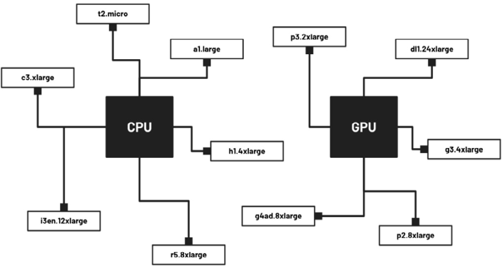
Figure 2.8 – CPU instances versus GPU instances

That said, we need to identify which instances fall under the group of GPU instances and which instances fall under the CPU instances umbrella. The preceding diagram shows some examples of GPU instances, including p3.2xlarge, dl1.24xlarge, g3.4xlarge, p2.8xlarge, and g4ad.8xlarge. There are other examples of GPU instance types not in this list, but you should be able to identify these just by checking the instance family. For example, we are sure that p3.8xlarge is a GPU instance type since it belongs to the same family as the p3.2xlarge instance type.

Now that we have a better idea of what CPU and GPU instances are, let’s proceed with locating and choosing p3.2xlarge from the list of options for our instance type:

1. Continuing where we left off in the Locating the framework-specific DLAMI section, let’s locate and click the Compare instance types link under the Instance type pane. This should redirect you to the Compare instance types page, as shown in the following screenshot:

Figure 2.9 – Compare instance types

Here, we can see the different instance types, along with their corresponding specs and cost per hour.

2. Click the search field (with the Filter instance types placeholder text). This should open a drop-down list of options, as shown in the following screenshot:

Figure 2.10 – Using the Filter instance types search field

Locate and select GPUs from the list of options. This should open the Add filter for GPUs window.

3. In the Add filter for GPUs window, open the dropdown menu and select > from the list of options available. Next, specify a value of 0 in the text field beside it. Click the Confirm button afterward.

Note

The filter we applied should limit the set of results to GPU instances. We should find several accelerated computing instance families such as P3, P2, G5, G4dn, and G3, to name a few.

4. Next, let’s click the Preferences button, as highlighted in the following screenshot:

Figure 2.11 – Opening the Preferences window

This should open the Preferences window. Under Attribute columns, ensure that the GPUs radio button is toggled on, as shown in the following screenshot:

Figure 2.12 – Displaying the GPUs attribute column

Click the Confirm button afterward. This should update the table list display and show us the number of GPUs of each of the instance types in the list, as shown here:

Figure 2.13 – GPUs of each instance type

Here, we should see a pattern that the number of GPUs generally increases as the instance type becomes “larger” within the same instance family.

5. Locate and select the row corresponding to the p3.2xlarge instance type. Take note of the number of GPUs available, along with the cost per hour (on-demand Linux pricing) for the p3.2xlarge instance type.
6. Click the Select instance type button (located at the lower right portion of the screen) afterward.

This should close the Compare instance types window and return you to the Launch an instance page.

Ensuring a default secure configuration

When launching an EC2 instance, we need to manage the security configuration, which will affect how the instance will be accessed. This involves configuring the following:

• Key pair: Files containing credentials used to securely access the instance (for example, using SSH)
• Virtual Private Cloud (VPC): A logically isolated virtual network that dictates how resources are accessed and how resources communicate with each other
• Security group: A virtual firewall that controls traffic going in and out of the EC2 instance using rules that filter the traffic based on the configured protocol and ports

That said, let’s proceed with completing the remaining configuration parameters before we launch the EC2 instance:

1. Continuing where we left off in the Choosing the instance type section, let’s proceed with creating a new key pair. Under Key pair (login), locate and click Create new key pair.
2. In the Create key pair window, specify a unique key pair name (for example, dlami-key) for Key pair name. Ensure that the following configuration holds as well:
   • Key pair type: RSA
   • Private key file format: .pem
3. Click the Create key pair button afterward. This should automatically download the .pem file to your local machine. Note that we won’t need this .pem file for the hands-on solutions in this chapter since we’ll be accessing the instance later using EC2 Instance Connect (through the browser).

Important Note

Never share the downloaded key file since this is used to access the instance via SSH. For production environments, consider hiding non-public instances inside a properly configured VPC as well. There’s a lot to discuss when it comes to securing our ML environments. We will talk about security in detail in Chapter 9, Security, Governance, and Compliance Strategies.

4. Under Network settings, locate and click the Edit button (located at the top right of the pane). Make sure that the following configuration settings are applied:
   • VPC - required: [Select default VPC] vpc-xxxxxxxx (default)
   • Auto-assign public IP: Enable
   • Firewall (security groups): Create security group
5. Under Inbound security group rules of Network settings, specify a set of security group rules, similar to what is configured in the following screenshot:

Figure 2.14 – Inbound security groups rules

As you can see, we will be configuring the new security group with the following rules:

• Type: SSH; Protocol: TCP; Port Range: 22; Source type: Anywhere | Source: 0.0.0.0/0; Description: SSH – allows any “computer” such as your local machine to connect to the EC2 instance via the Secure Shell (SSH) protocol over port 22
• Type: Custom TCP; Protocol: TCP; Port Range: 6006; Source type: Anywhere | Source: 0.0.0.0/0; Description: Tensorboard – allows any “computer” such as your local machine to access port 6006 of the EC2 instance (which may be running an application such as TensorBoard)
• Type: Custom TCP; Protocol: TCP; Port Range: 8888; Source type: Anywhere | Source: 0.0.0.0/0; Description: Jupyter – allows any “computer” such as your local machine to access port 8888 of the EC2 instance (which may be running an application such as the Jupyter Notebook app)

You may proceed with the next step once you have configured the new security group with Security group name – required and Description – required and the relevant set of Inbound security group rules.

Note

Note that this configuration needs to be reviewed and secured further once we need to prepare our setup for production use. For one, Source type for any of these security group rules should not have been set to Anywhere (0.0.0.0/0) since this configuration allows any computer or server to access our instance through the open ports. That said, we could have limited access to only the IP address of our local machine. In the meantime, the configuration we have should do the trick since we will delete the instance immediately once we have completed this chapter.

6. Locate and click the Add new volume button under Configure storage:

Figure 2.15 – Configuring the storage settings

Specify 35 in the text field between 1x and GiB. similar to what we have in the preceding screenshot.

There are a few more options we can configure and tweak (under Advanced Details) but we’ll leave the default values as-is.

Launching the instance and connecting to it using EC2 Instance Connect

There are different ways to connect to an EC2 instance. Earlier, we configured the instance so that it can be accessed via SSH using a key file (for example, from the Terminal of your local machine). Another possible option is to use EC2 Instance Connect to access the instance through the browser. We can also access the instance via SSH using Session Manager. In this section, we’ll use EC2 Instance Connect to access our instance.

Continuing where we left off in the Ensuring a default secure configuration section, let’s proceed with launching the EC2 instance and access it from the browser:

1. Once you have configured the storage settings, locate and click the Launch instance button under the Summary pane (located at the right portion of the screen). Make sure that you terminate this instance within the hour it has been launched as the per-hour rate of these types of instances is a bit higher relative to other instance types. You may check the Cleaning up section of this chapter for more details.

Note

Make sure that the value specified in the Number of instances field is set to 1. Technically, we can launch 20 instances all in one go by setting this value to 20. However, we don’t want to do this as this would be very expensive and wasteful. For now, let’s stick to 1 as this should be more than enough to handle the deep learning experiments in this chapter.

2. You should see a success notification, along with the instance ID of the resource being launched, similar to what is shown in the following screenshot:

Figure 2.16 – Launch success notification

Click the link containing the instance ID (i-xxxxxxxxxxxxxxxxx), as highlighted in the preceding screenshot, to navigate to the Instances page. You may click the refresh button (beside the Connect button) a few times while waiting for the EC2 instance (MLE-CH02-DLAMI) to appear in the list of instances.

Note

Wait for a minute or two before proceeding with the next step. In case you experience an InsufficientInstanceCapacity error while launching the instance, feel free to use a different p3 instance. To troubleshoot this further, you may also refer to https://aws.amazon.com/premiumsupport/knowledge-center/ec2-insufficient-capacity-errors/ for more information.

3. Select the instance by toggling the checkbox highlighted in the following screenshot. Click the Connect button afterward:

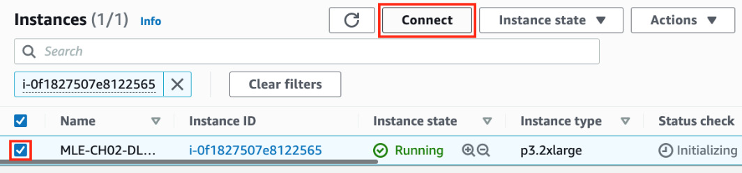
Figure 2.17 – Connecting to the instance directly

Here, we can see that there’s an option to connect directly to the instance using the browser.

4. In the EC2 Instance Connect tab, locate and copy the Public IP address value (AA.BB.CC.DD) to a text editor on your local machine. Note that you will get a different public IP address value. We will use this IP address value later in this chapter when accessing TensorBoard (the visualization toolkit of TensorFlow) and the Jupyter notebook application. Leave the User name value as-is (root) and then click Connect:

Figure 2.18 – EC2 Instance Connect

This should open a new tab that will allow us to run terminal commands directly from the browser. If you are getting a There was a problem connecting to your instance error message, wait for about 2 to 3 minutes before refreshing the page or clicking the Retry button:

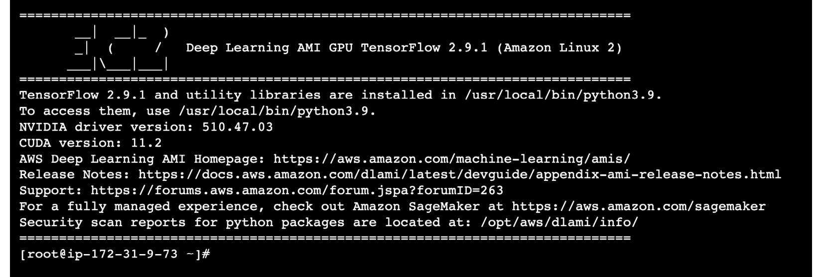
Figure 2.19 – EC2 Instance Connect terminal

As we can see, TensorFlow 2.9.1 and other utility libraries are installed in /usr/local/bin/python3.9. Note that you may get different TensorFlow and Python versions, depending on the version of the DLAMI you use to launch the instance.

Wasn’t that easy? At this point, we should now be able to perform deep learning experiments using TensorFlow without having to install additional tools and libraries inside the EC2 instance.

Note

Note that this process of launching instances from AMIs can be further sped up using Launch Templates, which already specify instance configuration information such as the AMI ID, instance type, key pair, and security groups. We won’t cover the usage of Launch Templates in this book, so feel free to check the following link for more details: https://docs.aws.amazon.com/AWSEC2/latest/UserGuide/ec2-launch-templates.html.

Downloading the sample dataset

In the succeeding sections of this chapter, we will work with a very simple synthetic dataset that contains only two columns – x and y. Here, x may represent an object’s relative position on the X-axis, while y may represent the same object’s position on the Y-axis. The following screenshot shows an example of what the data looks like:

Figure 2.20 – Sample dataset

ML is about finding patterns. With this dataset, we will build a model that tries to predict the value of y given the value of x later in this chapter. Once we’re able to build models with a simple example like this, it will be much easier to deal with more realistic datasets that contain more than two columns, similar to what we worked with in Chapter 1, Introduction to ML Engineering on AWS.

Note

In this book, we won’t limit ourselves to just tabular data and simple datasets. In Chapter 6, SageMaker Training and Debugging Solutions, for example, we’ll work with labeled image data and build two image classification models using several capabilities and features of Amazon SageMaker. In Chapter 7, SageMaker Deployment Solutions, we’ll work with text data and deploy a natural language processing (NLP) model using a variety of deployment options.

That said, let’s continue where we left off in the Launching the instance and connecting to it using EC2 Instance Connect section and proceed with downloading the dataset we will use to train the deep learning model in this chapter:

1. In the EC2 Instance Connect window (or tab), run the following command to create the data directory:

   mkdir -p data
2. Download the training, validation, and test datasets using the wget command:

   wget https://bit.ly/3h1KBx2 -O data/training_data.csv
   wget https://bit.ly/3gXYM6v -O data/validation_data.csv
   wget https://bit.ly/35aKWem -O data/test_data.csv
3. Optionally, we can install the tree utility using the yum package management tool:

   yum install tree

If this is your first time encountering the tree command, it is used to list the directories and files in a tree-like structure.

Note

It is also possible to create a custom AMI from an EC2 instance. If we were to create a custom AMI from the EC2 instance we are using right now, we would be able to launch new EC2 instances from the new custom AMI with the following installed already: (1) installed frameworks, libraries, and tools from the DLAMI, and (2) the tree utility we installed before the custom AMI was created.

4. Use the tree command to see the current set directories and files in the current directory:

   tree

This should yield a tree-like structure, similar to what is shown in the following screenshot:

Figure 2.21 – Results after using the tree command

Here, we can see that we have successfully downloaded the CSV files using the wget command earlier.

5. Now, let’s verify and check the contents of one of the CSV files we have downloaded. Use the head command to see the first few rows of the training_data.csv file:

   head data/training_data.csv

This should give us rows of (x,y) pairs, similar to what is shown in the following screenshot:

Figure 2.22 – The first few rows of the training_data.csv file

You may check the contents of validation_data.csv and test_data.csv using the head command as well.

Note

It is important to note that the first column in this example is the y column. Some ML practitioners follow a convention where the first column is used as the target column (the column containing the values we want to predict using the other columns of the dataset). When using certain algorithms such as the XGBoost and Linear Learner built-in algorithms of SageMaker, the first column is assumed to be the target column. If you are using your own custom scripts to load the data, you can follow any convention you would like since you have the freedom of how the data is loaded and interpreted from a file.

You have probably noticed by now that, so far in this book, we have been using clean and preprocessed datasets. In real ML projects, you’ll be dealing with raw data with a variety of issues such as missing values and duplicate rows. In Chapter 5, Pragmatic Data Processing and Analysis, we’ll be working with a “dirtier” version of the bookings dataset and use a variety of AWS services and capabilities such as AWS Glue DataBrew and Amazon SageMaker Data Wrangler to analyze, clean, and process the data. In this chapter, however, we will work with a “clean” dataset since we need to focus on training a deep learning model using TensorFlow and Keras. That said, let’s proceed with generating a model that accepts x as the input and returns a predicted y value as the output.

Training an ML model

In Chapter 1, Introduction to ML Engineering on AWS, we trained a binary classifier model that aims to predict if a hotel booking will be canceled or not using the available information. In this chapter, we will use the (intentionally simplified) dataset from Downloading the Sample Dataset and train a regression model that will predict the value of y (continuous variable) given the value of x. Instead of relying on ready-made AutoML tools and services, we will be working with a custom script instead:

Figure 2.23 – Model life cycle

When writing a custom training script, we usually follow a sequence similar to what is shown in the preceding diagram. We start by defining and compiling a model. After that, we load the data and use it to train and evaluate the model. Finally, we serialize and save the model into a file.

Note

What happens after the model has been saved? The model file can be used and loaded in an inference endpoint — a web server that uses a trained ML model to perform predictions (for example, predicted y values) given a set of input values (for example, input x values). In the Loading and evaluating the model section of this chapter, we’ll load the generated model file inside a Jupyter Notebook using the load_model() function from tf.keras.models. We’ll then use the predict() method to perform sample predictions using a provided test dataset.

In this chapter, we will work with a script file that uses TensorFlow and Keras to build a neural network model – an interconnected group of nodes that can learn complex patterns between inputs and outputs. As we will be working with neural networks and deep learning concepts in this book, we must have a basic understanding of the following concepts:

• Neurons: These are the building blocks of neural networks that accept and process input values to produce output values. How are the output values computed? Each of the input values passing through the neuron is multiplied by the associated weight values and then a numerical value (also known as the bias) is added afterward. A non-linear function called the activation function is then applied to the resulting value, which would yield the output. This non-linear function helps neural networks learn complex patterns between the input values and the output values. We can see a representation of a neuron in the following diagram:

Figure 2.24 – A representation of a neuron

Here, we can see that we can compute the value of y with a formula involving the x input values, the corresponding weight values, the bias, and the activation function. That said, we can think of a neuron as a “mathematical function” and a neural network as a “bunch of mathematical functions” trying to map input values with output values through the continuous update of weight and bias values.

• Layers: Layers are composed of a group of neurons located at a specific location or depth in a neural network:

Figure 2.25 – An input layer, output layer, and multiple hidden layers

Here, we can see the different layers of a neural network. The input layer is the layer receiving the input values, while the output layer is the layer generating the output values. Between the input layer and the output layer are processing layers called hidden layers, which process and transform the data from the input layer to the output layer. (Neural networks with more than one or two hidden layers are generally called deep neural networks.)

• Forward propagation: This refers to the forward flow of information from the input layer to the hidden layers and then to the output layers to generate the output values.
• Cost function: This function is used to compute how far off the predicted computed value is from the actual value. Given that the goal of training a neural network is to generate a predicted value as close as possible to the actual value, we should be aiming to look for a minimum value of the cost function (which represents the error of the model) using optimization algorithms such as Gradient Descent.
• Backpropagation: This is the process of adjusting the weights in a neural network based on the difference between the predicted values and the actual values (which involves calculating the gradients or making small updates to the weights in each layer):

Figure 2.26 – Backpropagation

Here, we can see that backpropagation involves propagating the computed error backward from the output layer to the input layer (and updating the weights accordingly).

• Learning rate: This influences the amount used to adjust the weights in the network concerning the loss gradient while training the neural network.
• Epoch: This is a training iteration that involves one forward and one backward propagation using the entire training dataset. After each training iteration, the weights of the neural network are updated, and the neural network is expected to perform better in mapping the set of input values into the set of output values.

Note

We won’t dive deep into the details of deep learning and neural networks in this book. If you are interested in learning more about these topics, there are several books available online: https://www.amazon.com/Neural-Network/s?k=Neural+Network.

Now that we have a better idea of what neural networks are, we can proceed with training a neural network model. In the next set of steps, we will use a custom script to train a deep learning model with the data downloaded in the previous section:

1. First, let’s create a directory named logs using the mkdir command:

   mkdir -p logs
2. Next, use the wget command to download the train.py file:

   wget https://bit.ly/33D0iYC -O train.py
3. Use the tree command to quickly check what the file and directory structure looks like:

   tree

This should yield a tree-like structure, similar to what is shown in the following screenshot:

Figure 2.27 – Results after using the tree command

Note that the data and log directories are at the same level as the train.py file.

4. Before running the train.py file, execute the following command:

   for a in /sys/bus/pci/devices/*; do echo 0 | sudo tee -a $a/numa_node; done

This will help us avoid the successful NUMA node read from SysFS had negative value (-1) warning message when listing the GPU devices later in this chapter.

5. Before running the downloaded train.py script, let’s check its contents by opening https://github.com/PacktPublishing/Machine-Learning-Engineering-on-AWS/blob/main/chapter02/train.py in a separate browser tab:

Figure 2.28 – The train.py file

In the preceding screenshot, we can see that our train.py script does the following:

• (1) defines a sample neural network model using the prepare_model() function
• (2) loads the training and validation data using the load_data() function
• (3) prepares the TensorBoard callback object
• (4) performs the training step using the fit() method and passes the TensorBoard callback object as the callback parameter value
• (5) saves the model artifacts using the save() method

Note

It is important to note that the prepare_model() function in our train.py script performs both the define model and compile model steps. The neural network defined in this function is a sample sequential model with five layers. For more information, feel free to check out the implementation of the prepare_model() function at https://github.com/PacktPublishing/Machine-Learning-Engineering-on-AWS/blob/main/chapter02/train.py.

6. Let’s start the training step by running the following in the EC2 Instance Connect terminal:

   python3.9 train.py

This should yield a set of logs, similar to what is shown in the following screenshot:

Figure 2.29 – train.py script logs

Note that the training step may take around 5 minutes to complete. Once the train.py script has finished executing, you may check the new files generated inside the logs and model directories using the tree command.

Note

What’s happening here? Here, the fit() method of the model we defined in train.py is training the model with the number of epochs (iterations) set to 500. For each iteration, we are updating the weights of the neural network to minimize the “error” between the actual values and the predicted values (for example, using cross-validation data).

7. Next, run the following command to run the tensorBoard application, which can help visualize and debug ML experiments:

   tensorboard --logdir=logs --bind_all
8. Open a new browser tab and open TensorBoard by going to http://<IP ADDRESS>:6006. Replace <IP ADDRESS> with the public IP address we copied to our text editor in the Launching an EC2 instance using a Deep Learning AMI section:

Figure 2.30 – TensorBoard

This should load a web application, similar to what is shown in the preceding screenshot. We won’t dive deep into what we can do with TensorBoard, so feel free to check out https://www.tensorflow.org/tensorboard for more information.

Note

How do we interpret these charts? As shown in Figure 2.30, the training and validation loss generally decrease over time. In the first chart (top), the X-axis corresponds to the epoch number, while the Y-axis shows the training and validation loss. It should be noted that in this chart, the train and validation “learning curves” are overlapping and both continue to decrease up to a certain point as the number of epochs or iterations increases. It should be noted that these types of charts help diagnose ML model performance, which would be useful in avoiding issues such as overfitting (where the trained model performs well on the training data but performs poorly on unseen data) and underfitting (where the trained model performs poorly on the training dataset and unseen data). We won’t discuss this in detail, so feel free to check other ML and deep learning resources available.

9. Navigate back to the EC2 Instance Content terminal and stop the running TensorBoard application process with Ctrl + C.

At this point, we should have the artifacts of a trained model inside the model directory. In the next section, we will load and evaluate this model inside a Jupyter Notebook environment.

Loading and evaluating the model

In the previous section, we trained our deep learning model using the terminal. When performing ML experiments, it is generally more convenient to use a web-based interactive environment such as the Jupyter Notebook. We can technically run all the succeeding code blocks in the terminal, but we will use the Jupyter Notebook instead for convenience.

In the next set of steps, we will launch the Jupyter Notebook from the command line. Then, we will run a couple of blocks of code to load and evaluate the ML model we trained in the previous section. Let’s get started:

1. Continuing where we left off in the Training an ML model section, let’s run the following command in the EC2 Instance Connect terminal:

   jupyter notebook --allow-root --port 8888 --ip 0.0.0.0

This should start the Jupyter Notebook and make it accessible through port 8888:

Figure 2.31 – Jupyter Notebook token

Make sure that you copy the generated random token from the logs generated after running the jupyter notebook command. Refer to the preceding screenshot on where to get the generated token.

2. Open a new browser tab and open the Jupyter application by accessing http://<IP ADDRESS>:8888. Replace <IP ADDRESS> with the public IP address we copied to our text editor in the Launching an EC2 instance using a Deep Learning AMI section:

Figure 2.32 – Accessing the Jupyter Notebook

Here, we can see that we are required to input a password or token before we can use the Jupyter Notebook. Simply input the token obtained from the logs generated in the previous step.

Important Note

Note that this setup is not ready for use in production environments. For more information on how to secure the Jupyter Notebook server, check out https://jupyter-notebook.readthedocs.io/en/stable/security.html. We will also discuss a few strategies to improve the security of this setup in Chapter 9, Security, Governance, and Compliance Strategies.

3. Create a new notebook by clicking New and selecting Python 3 (ipykernel) from the list of dropdown options, similar to what is shown in the following screenshot:

Figure 2.33 – Creating a new Jupyter Notebook

This should open a blank notebook where we can run our Python code.

4. Import tensorflow and then use list_physical_devices() to list the visible GPUs in our instance:

   import tensorflow as tf
   tf.config.list_physical_devices('GPU')

This should return a list with a single PhysicalDevice object, similar to [PhysicalDevice(name='/physical_device:GPU:0',device_type='GPU')].

Note

Since we are using a p3.2xlarge instance, the preceding block of code returned a single visible GPU device. If we launched a p3.16xlarge instance, we should get 8 visible GPU devices instead. Note that we can significantly reduce the training time by utilizing multiple GPU devices at the same time through parallelism techniques such as data parallelism (where the same model is used in each GPU but trained with different chunks of the dataset) and model parallelism (where the model is divided into several parts equal to the number of GPUs). Of course, the ML experiment scripts need to be modified to utilize multiple GPUs. For more information on how to use a GPU in TensorFlow, feel free to check the following link for more details: https://www.tensorflow.org/guide/gpu.

5. Load the model using tf.keras.models.load_model(). Inspect the model using model.summary():

   model = tf.keras.models.load_model('model')
   model.summary()

This should yield a model summary, as shown in the following screenshot:

Figure 2.34 – Model summary

This model summary should reflect the properties of the model we prepared and trained in the Training an ML model section.

Important Note

Make sure to load only ML models from trusted sources using the load_model() function (along with other similar functions). Attackers can easily prepare a model (with a malicious payload) that, when loaded, will give the attacker access to the server running the ML scripts (for example, through a reverse shell). For more information on this topic, you may check the author’s talk on how to hack and secure ML environments and systems: https://speakerdeck.com/arvslat/pycon-apac-2022-hacking-and-securing-machine-learning-environments-and-systems?slide=21.

6. Define the load_data() function, which will return the values of a CSV file with the specified file location:

   import numpy as np
   def load_data(training_data_location):
       fo = open(training_data_location, "rb")
       result = np.loadtxt(fo, delimiter=",")
       
       y = result[:, 0]
       x = result[:, 1]
       
       return (x, y)
7. Now, let’s test if the loaded model can perform predictions given as a set of input values. Load the test data using load_data() and perform a few sample predictions using model.predict():

   x, y = load_data("data/test_data.csv")
   predictions = model.predict(x[0:5])
   predictions

This should yield an array of floating-point values, similar to what is shown in the following screenshot:

Figure 2.35 – Prediction results

Here, we have the array of predicted y target values that correspond to each of the five input x values. Note that these predicted y values are different from the actual y values loaded from the test_data.csv file.

8. Evaluate the loaded model using model.evaluate():

   results = model.evaluate(x, y, batch_size=128)
   results

This should give us a value similar to or close to 2.705784797668457. If you are wondering what this number means, this is the numerical value corresponding to how far the predicted values are from the actual values:

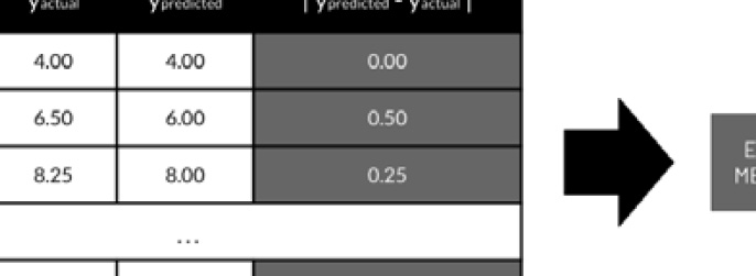
Figure 2.36 – How model evaluation works

Here, we can see an example of how model evaluation works for regression problems. First, evaluation metrics such as Root Mean Square Error (RMSE), Mean Square Error (MSE), and Mean Absolute Error (MAE) compute the differences between the actual and predicted values of y before computing for a single evaluation metric value. This means that a model with a lower RMSE value generally makes fewer mistakes compared to a model with a higher RMSE value.

At this point, you may decide to build a custom backend API utilizing the preceding blocks of code, along with Python web frameworks such as Flask, Pyramid, or Django. However, you may want to check other built-in solutions first, such as TensorFlow Serving (an ML model serving system for TensorFlow models), which is designed for production environments.

If you think about it, we have completed an entire ML experiment in the last couple of sections without having to install any additional libraries, packages, or frameworks (other than the optional tree utility). With that, you have learned how useful and powerful Deep Learning AMIs are! Again, if we had to set up 20 or more ML environments like this, it would take us maybe less than 2 hours to get everything set up and ready.

Cleaning up

Now that we have completed an end-to-end ML experiment, it’s about time we perform the cleanup steps to help us manage costs:

1. Close the browser tab that contains the EC2 Instance Connect terminal session.
2. Navigate to the EC2 instance page of the instance we launched using the Deep Learning AMI. Click Instance state to open the list of dropdown options and then click Terminate instance:

Figure 2.37 – Terminating the instance

As we can see, there are other options available, such as Stop instance and Reboot instance. If you do not want to delete the instance yet, you may want to stop the instance instead and start it at a later date and time. Note that a stopped instance will incur costs since the attached EBS volume is not deleted when an EC2 instance is stopped. That said, it is preferable to terminate the instance and delete any attached EBS volume if there are no critical files stored in the EBS volume.

3. In the Terminate instance? window, click Terminate. This should delete the EC2 instance, along with the volume attached to it.

Unused resources should be turned off, terminated, or deleted when no longer needed to manage and reduce costs. As our ML and ML engineering requirements need more resources, we will have to make use of several cost optimization strategies to manage costs. We will discuss some of these strategies in the next section.

Understanding how AWS pricing works for EC2 instances

Before we end this chapter, we must have a good idea of how AWS pricing works when dealing with EC2 instances. We also need to understand how the architecture and setup affect the overall cost of running ML workloads in the cloud.

Let’s say that we initially have a single p2.xlarge instance running 24/7 for an entire month in the Oregon region. Inside this instance, the data science team regularly runs a script that trains a deep learning model using the preferred ML framework. This training script generally runs for about 3 hours twice every week. Given the unpredictable schedule of the availability of new data, it’s hard to know when the training script will be run to produce a new model. The resulting ML model then gets deployed immediately to a web API server, which serves as the inference endpoint within the same instance. Given this information, how much would the setup cost?

Figure 2.38 – Approximate cost of running a p2.xlarge instance per month

Here, we can see that the total cost for this setup would be around at least $648 per month. How were we able to get this number? We start by looking for the on-demand cost per hour of running a p2.xlarge instance in the Oregon region (using the following link as a reference: https://aws.amazon.com/ec2/pricing/on-demand/). At the time of writing, the on-demand cost per hour of a p2.xlarge instance would be $0.90 per hour in the Oregon (us-west-2) region. Since we will be running this instance 24/7 for an entire month, we’ll have to compute the estimated total number of hours per month. Assuming that we have about 30 days per month, we should approximately have a total of 720 hours in a single month – that is, 24 hours per day x 30 days = 720 hours.

Note that we can also use 730.001 hours as a more accurate value for the total number of hours per month. However, we’ll stick with 720 hours for now to simplify things a bit. The next step is to multiply the cost per hour of running the EC2 instance ($0.90 per hour) and the total number of hours per month (720 hours per month). This would give us the total cost of running the EC2 instance in a single month ($0.90 x 720 = $648).

Note

To simplify the computations in this section, we will only consider the cost per hour of using the EC2 instances. In real life, we’ll need to take into account the costs associated with using other resources such as the EBS volumes, VPC resources (NAT gateway), and more. For a more accurate set of estimates, make sure to use the AWS Pricing Calculator: https://calculator.aws/.

After a while, the data science team decided to train another model inside the same instance where we are already running a training script and a web server (inference endpoint). Worried that they might encounter performance issues and bottlenecks while running the two training scripts at the same time, the team requested for the p2.xlarge instance to be upgraded to a p2.8xlarge instance. Given this information, how much would the new setup cost?

Figure 2.39 – Approximate cost of running a p2.8xlarge instance per month

Here, we can see that the total cost for this setup would be around at least $5,184 per month. How were we able to get this number? We must follow a similar set of steps as with the previous example and look for the on-demand cost per hour of running a p2.8xlarge instance. Here, we can see that the cost of running a p2.8xlarge instance ($7.20 per hour) is eight times the cost of running a p2.xlarge instance ($0.90 per hour). That said, we’re expecting the overall cost to be eight times as well compared to the original setup that we had earlier. After multiplying the cost per hour of running the p2.8xlarge instance ($7.20 per hour) and the total number of hours per month (720 hours per month), we should get the total cost of running the p2.8xlarge instance in a single month ($7.20 x 720 = $5,184).

Using multiple smaller instances to reduce the overall cost of running ML workloads

At this point, you might be wondering if there is a better way to set things up to significantly lower the cost while running the same set of ML workloads. The good news is that there’s a variety of ways to improve what we have so far and reduce the cost from $5,184 per month to a much smaller value such as $86.40 per month! Note that this is also significantly smaller compared to the cost of running the original setup ($648 per month). How do we do this?

The first thing we need to do is utilize multiple “smaller” instances instead of a single p2.8xlarge instance. One possible setup is to use a p2.xlarge instance ($0.90 per hour) for each of the training scripts. Since we are working with two training scripts, we’ll have a total of two p2.xlarge instances. In addition to this, we’ll be using an m6i.large instance ($0.096 per hour) to host the inference endpoint where the model is deployed. Since the training scripts are only expected to run when there’s new data available (approximately twice per week), we can have p2.xlarge instances running only when we need to run the training scripts. This means that if we have around 720 hours per month, a p2.xlarge instance associated with one of the training scripts should only run for about 24 hours per month in total (with the instance turned off the majority of the time).

Note

How did we get this number? Since the training script is expected to run for about 3 hours twice every week, then the formula would be [3 hours per run] x [2 times per week] x [4 weeks], which would yield a value of 24 hours. This means that each of the p2.xlarge instances would cost around $21.60 per month if these would only run for a total of about 24 hours in a single month.

Even if these p2.xlarge instances are turned off most of the time, our ML inference endpoint would still be running 24/7 in its dedicated m6i.large instance. The cost of running the m6i.large instance for an entire month would be around $69.12 per month (using the [$0.096 per hour] x [720 hours per month] formula):

Figure 2.40 – Using multiple smaller instances to reduce the overall cost

That said, we should be able to reduce the overall cost to around $112.32 per month, similar to what is shown in the preceding diagram. How were we able to get this number? We simply added the expected costs of running each instance in a month: $21.60 + $21.60 + $69.12 = $112.32.

Using spot instances to reduce the cost of running training jobs

It is important to note that we can further decrease this cost by utilizing spot instances instead of on-demand instances for the p2.xlarge instances used to run the training scripts. With spot instances, we can reduce the cost of using a specific EC2 instance type by around 60% to 90% by utilizing the spare compute capacity available in AWS. This means that instead of paying $0.90 per hour when running p2.xlarge instances, we may only pay $0.36 per hour, assuming that we’ll have around 60% savings using spot instances. What’s the catch when using spot instances? When using spot instances, there’s a chance for the applications running inside these instances to be interrupted! This means that we should only run tasks (such as ML training jobs) that can be resumed after an unexpected interruption.

Note

How did we get this number? 60% savings is equivalent to multiplying the on-demand cost per hour ($0.90 per hour) by 0.40. This would give us [$0.90 per hour] x [0.40] = [$0.36 per hour].

Since interruptions are possible when using spot instances, it is not recommended that you use them for the 24/7 m6i.large instance where the web server (inference endpoint) is running:

Figure 2.41 – Using spot instances to reduce the cost of running training jobs

Once we’ve utilized spot instances for the p2.xlarge instances, we’ll be able to reduce the overall cost to around $86.40 per month, similar to what we have in the preceding diagram. Again, this final value excludes the other costs to simplify the computations a bit. However, as you can see, this value is significantly smaller than the cost of running a single p2.8xlarge instance ($5,184 per month).

Wasn’t that amazing?! We just changed the architecture a bit and we were able to reduce the cost from $5,184 per month to $86.40 per month! Note that there are other ways to optimize the overall costs of running ML workloads in the cloud (for example, utilizing Compute Savings Plans). What you learned in this section should be enough for now as we’ll continue with these types of discussions over the next few chapters of this book.

Summary

In this chapter, we were able to launch an EC2 instance using a Deep Learning AMI. This allowed us to immediately have an environment where we can perform our ML experiments without worrying about the installation and setup steps. We then proceeded with using TensorFlow to train and evaluate our deep learning model to solve a regression problem. We wrapped up this chapter by having a short discussion on how AWS pricing works for EC2 instances.

In the next chapter, we will focus on how AWS Deep Learning Containers help significantly speed up the ML experimentation and deployment process.

Further reading

We are only scratching the surface of what we can do with Deep Learning AMIs. In addition to the convenience of having preinstalled frameworks, DLAMIs make it easy for ML engineers to utilize other optimization solutions such as AWS Inferentia, AWS Neuron, distributed training, and Elastic Fabric Adapter. For more information, feel free to check out the following resources:

• What is the AWS Deep Learning AMI? (https://docs.aws.amazon.com/dlami/latest/devguide/what-is-dlami.html)
• How AWS Pricing Works (https://docs.aws.amazon.com/whitepapers/latest/how-aws-pricing-works/how-aws-pricing-works.pdf)
• Elastic Fabric Adapter (https://docs.aws.amazon.com/dlami/latest/devguide/tutorial-efa.html)