6

Batch Model Serving

The batch model serving pattern is more common than real-time serving in today’s world of large-scale data. With batch model serving, newly arrived data will not be immediately available in the model. Depending on the batching criteria, the impact of new data may become apparent after a certain period of time, ranging from an hour to a year. Batch model serving uses a large amount of data to build a model. This gives us a more robust and accurate model. On the other hand, as the batch model does not use live data, it cannot provide up-to-date information during prediction. For example, let’s consider a product recommendation model that recommends shirts, and the model is retrained at the end of every month. You will get a very accurate shirt recommendation based on the available shirts up to the last month, but if you are interested in shirts that have recently appeared on the market, this model will frustrate you, as it doesn’t have information about the most recent products. Therefore, we see that during batch serving, selecting the ideal batching criteria is a research topic that can be adjusted based on customer feedback.

In this chapter, we will discuss batch model serving. After completing this chapter, you will know what batch model serving is, and you will have seen some example scenarios of batch serving. The topics that will be covered in this chapter are listed here:

• Introducing batch model serving
• Different types of batch model serving
• Example scenarios of batch model serving
• Techniques in batch model serving

Technical requirements

In this chapter, we will discuss batch model serving, along with some example code. To run the code, please go to the Chapter 6 folder in the GitHub repository for the book and try to follow along: https://github.com/PacktPublishing/Machine-Learning-Model-Serving-Patterns-and-Best-Practices/tree/main/Chapter%206.

We shall be using cron expressions to schedule batch jobs in this chapter. The cron commands that will be run in this chapter need a Unix or Mac operating system (OS). If you are using Windows, you can use a virtual machine to run a Unix OS inside the virtual machine. Use this link to learn about some virtual machines for Windows: https://www.altaro.com/hyper-v/best-vm-windows-10/.

Introducing batch model serving

In this section, we will introduce the batch model serving pattern and give you a high-level overview of what batch serving is and why it is beneficial. We will also discuss some example cases that illustrate when batch serving is needed.

What is batch model serving?

Batch model serving is the mechanism of serving a machine learning model in which the model is retrained periodically using the saved data from the last period, and inferences are made offline and saved for quick access later on.

We do not retrain the model immediately when the data changes or new data arrives. This does not follow the CI/CD trend in web application serving. In web application serving, every change in the code or feature triggers a new deployment through the CI/CD pipeline. This kind of continuous deployment is not possible in batch model serving. Rather, the incoming data is batched and stored in persistent storage. After a certain amount of time, we add the newly collected data to the training data for the next update of the model.

This is also known as offline model serving, as the model does not represent recent data and the training and inference are usually done offline. By offline, here, we mean that the training and inference are done before the predictions are made available to the client. This time gap between training and using the inference is higher than the acceptable latency requirements for online serving, as clients can’t wait this long for a response after the request is made.

To understand batch model serving, first, let’s discuss two metrics that are crucial to serving and also to the monitoring of the health of serving. These metrics are as follows:

• Latency
• Throughput

Latency

Latency is the difference between the time a user makes a request and the time the user gets the response. The lower the latency, the better the client satisfaction.

For example, let’s say a user makes an API call at time T1 and gets the response at time T2.

Then, the latency is T2 – T1.

If the latency is high, then the application cannot be served online because there is a maximum timeout limit for an HTTP connection. By default, the value is set to 30 seconds and the maximum value is 5 minutes. However, in an ideal situation, we expect the response to be within milliseconds. AWS API Gateway sets a hard limit of 29 seconds before you encounter an error:

{
Message: "Endpoint request timed out"
}

Therefore, high latency discourages serving applications to the users.

Because of this latency constraint, we can understand why batch inference can’t serve the most recent large volumes of data. The modeling (training and evaluation) and inference will take a lot of time, and completing everything before this HTTP timeout period expires is not possible if the data volume is high and the inference needs heavy computation. That’s why in batch serving, we need to sacrifice latency and get our inference after a certain period.

Throughput

Throughput is the number of requests served per unit of time. For example, let’s say 10 requests are successfully served in 2 seconds by a server. The throughput in this case is 10/2 = 5 requests per second. Therefore, we want high throughput from the served application. To achieve this, we can scale horizontally by adding more servers and using the high computation power in the servers.

From our discussion of latency and throughput, you may have noticed that during serving, the goal should be to minimize latency and maximize throughput. By minimizing latency, we ensure customers get the response quickly. If the response does not come quickly, the users will lose interest in using the application. By maximizing throughput, we ensure that more customers can be served at the same time. If throughput is low, customers will keep getting a "Too many requests" exception.

In batch model serving, we want to maximize the throughput so that large numbers of clients can get predictions. For example, let’s say one million customers are using an e-commerce site. All of them need to get their product recommendations at the same time.

During batch serving, we give priority to throughput. We want all the clients to get their predictions at the same time to ensure the fairness of service. However, we get the inference result a certain amount of time after the inference request is sent.

Main components of batch model serving

Batch model serving has three main components:

• Storing batch data in a persistent store: During batch model serving, we cannot use live data to update the model. We have to wait for a certain amount of time and retrain the model using the data. For that reason, we need to store the data in a persistent store and use the data from the persistent store to train the model. Sometimes, we might want to use the data only from a certain recent period of time. The database we choose depends on the amount of data we’re going to work with. It may be the case that it is sufficient to store the data in CSV files; it may also be necessary to move it to specialized databases for big data, such as Hadoop or Spark. We can organize the files or tables and separate them. For example, we can keep a separate table for each month, or we can keep a file for each genre in a movie or book recommendation model data.
• Trigger for retraining the model: We need to decide when the model will be retrained. This can be done manually through manual observations, it can be done automatically with scheduling, or the model can be retrained using the evaluation metric by using continuous evaluation, as discussed in Chapter 4, Continuous Model Evaluation.
• Releasing the latest inference to the server: After the model is trained and the inference is completed, we can then write the inference result to the database. However, we need to let the servers know that the update to the model is complete. Usually, we can follow a notification strategy to publish a notification with the information that the update is completed.

In this section, we have introduced batch serving to you. In the next section, we will see when to use different types of batch model serving based on different criteria. We will also introduce cron expressions for scheduling periodic batch jobs during batch model serving.

Different types of batch model serving

Batch model serving can be divided into a few categories with different parameters and settings. The characteristics that can create differences in batch model serving are as follows:

• Trigger mechanisms
• Batch data usage strategy
• Based on the inference strategy

We can classify batch model serving into three categories based on the trigger mechanism:

• Manual triggers
• Automatic periodic triggers
• Triggers based on continuous evaluation

Let’s look at each of them.

Manual triggers

With a manual trigger, the developer manually starts the retraining of the model and only then does the model start retraining using the most recent saved data. The developer team can keep monitoring the performance of the model to find out when the model needs retraining. The retraining decision can also come from the business users of the model. They can request the developer team for retraining and then the developer can retrain the model.

The manual trigger has the following advantages:

• Unnecessary computation can be avoided. As computation is not free, we can save a lot of money by avoiding periodic retraining unless the clients need the latest update.
• By deploying manually, the developers can observe and fix any problems arising during the training.

However, this approach has the following disadvantages:

• There is an added burden on the developer team to monitor the model’s performance and decide when retraining is needed
• Manual observation may be erroneous or biased

Let’s see how to monitor this in practice.

Monitoring for manual triggers

For manual observation, the developer team might need to conduct surveys to understand whether the clients are satisfied and are getting the desired predictions. The survey questions can be designed based on the model’s business goals. For example, for a product recommendation site, we can set up a survey where users rate how happy they are with their recommendations. We can then check the average rating and see that it is dropping every time. If the average rating approaches a certain threshold, the developers can retrain the model.

To see a code example of this, let’s say the developer sends surveys to five users every week and the survey responses are as follows:

Figure 6.1 – Rating submitted by five users over different weeks

In the table in Figure 6.1, the users’ ratings are collected over 5 different weeks. The users submit a rating out of five based on how satisfied the users are with their product recommendations. The developers can use this result to decide when they should start retraining the model. The deciding criteria can be whatever you want. For example, the following criteria may be used:

• When the average rating is <= 4.0, start retraining. In this case, the developers will start retraining in week 3.
• When the first rating of <= 3 comes in, start retraining. In that case, the developers will retrain in week 4.
• When the median rating is <= 3, then do the retraining. In that case, the developers will start retraining in week 5.

These criteria are dependent on the team. However, we can see from the criteria mentioned here that the training can happen in Week 3, Week 4, or Week 5.

We can use these conditions listed previously as flags that can indicate whether retraining should be done or not. We can compute the previously listed mentioned triggers in the following way:

import numpy as np
users = ["A", "B", "C", "D", "E"]
w1 = np.array([5, 5, 5, 5, 5])
w2 = np.array([5, 4, 4, 5, 5])
w3 = np.array([4, 4, 4, 4, 4])
w4 = np.array([3, 3, 4, 4, 4])
w5 = np.array([3, 3, 3, 3, 3])
def check_any_less_than_3(rating):
    mappedArray = rating <= 3
    return mappedArray.any()
print("Checking when first rating <= 3 appears")
print(check_any_less_than_3(w1))
print(check_any_less_than_3(w2))
print(check_any_less_than_3(w3))
print(check_any_less_than_3(w4))
print(check_any_less_than_3(w5))
def check_average(rating):
    mean = np.mean(rating)
    return mean <= 4.0
print("Checking when average rating becomes <= 4.0")
print(check_average(w1))
print(check_average(w2))
print(check_average(w3))
print(check_average(w4))
print(check_average(w5))
def check_median(rating):
    median = np.median(rating)
    return median <= 3.0
print("Checking when the median becomes <= 3.0")
print(check_median(w1))
print(check_median(w2))
print(check_median(w3))
print(check_median(w4))
print(check_median(w5))

From this code snippet, we get the following response:

Checking when first rating <= 3 appears
False
False
False
True
True
Checking when average rating becomes <= 4.0
False
False
True
True
True
Checking when the median becomes <= 3.0
False
False
False
False
True

In the response, we have highlighted when the trigger responds with True. We can see that True is returned in different weeks for different criteria, so if the business case is sensitive, the developers can choose the criterion that allows them to train the model as early as possible to ensure greater customer satisfaction. In that case, the developers can monitor both criteria and work on whichever comes first. If the business case does not require such tight accuracy, then the developers can use the criterion that gives them less pressure in terms of redeployment and reduce their computation costs.

Another approach to monitoring may be to keep a light model in parallel with the big model in production. The light model will be trained regularly for a limited number of randomly selected users. Then, we can monitor the inference of the model for those users in the production server and compare it with the inference made by the light model in the development server. For example, let’s consider the product recommendations for a user from a batch model and from a light model, which are shown in the table in Figure 6.2.

Figure 6.2 – Recommendations from the batch and light online model

We can now compute the Precision@k metric for the user from the two recommendations. For simplicity, let’s assume the current relevant items for the user are [Product 10, Product 9, Product 1, Product 2, Product 3]. However, the model in production shows three of these relevant items and two non-relevant items – so, in this case, P(k=5) = 3/5 = 60%. The developer will look at the value of this metric and identify that the model performance has degraded. Therefore, based on the result of a recommendation from the production server and the lightweight model in the development server, the developer can manually decide to trigger retraining.

Precision@k

Precision@k is the ratio of the total relevant results to the total recommended results in the top k recommended items. For example, let’s say a recommender system has made these recommendations: [R1, R2, R3, R4, R5]. However, among these recommendations, only R1, R3, and R4 are relevant to the user. In that case, Precision@5 is P(k=5) = 3/5. Here, we are considering the top 5 recommended products, so the value of k is 5.

Automatic periodic triggers

We can also periodically trigger the retraining using some periodic scheduler tools. For example, we can use cron expressions to set up cron jobs periodically.

Cron jobs

In Unix, cron is used to schedule periodic jobs using cron expressions. The job can run periodically at a fixed time, date, or interval. A cron expression that is used to schedule cron jobs can have five fields, as shown by the five asterisks in Figure 6.3.

Figure 6.3 – Cron expressions and their meanings (code screenshot captured from Wikipedia at https://en.wikipedia.org/wiki/Cron)

The fields are the following:

• minute: The first field is the minute field, which indicates the minute at which the job will run. If we keep the default value, *, then it will keep running every minute. We can replace * with a number, n, to denote that the job will run every n minutes. We can also have multiple minutes separated by commas. For example, if the minute field is n1, n2, n3, it means the job will be scheduled to run every n1, n2, and n3 minutes. We can also set a range using a hyphen (-) between the two numbers. For example, n1-n2 means the job will run every minute between n1 and n2.
• hour: The second field denotes the hour at which the job will run. If we keep the default value, *, then the job will run every hour. As with minutes, we can specify a number, comma-separated values of multiple numbers, or a range of numbers.
• day of the month: This specifies the day of the month on which the cron job will run. We can specify a single day, a comma-separated list of multiple days, or a range.
• month: This field specifies the month the cron job will run. We can specify a month, a list of months using commas, or a range of months.
• day of the week: This last field specifies the weekday on which a job will run. We can specify a particular weekday, a list of weekdays by separating the numbers with commas, or a range of weekdays.

Now, we can do some exercises to get some practice with cron expressions. You can learn more about cron expressions by visiting https://crontab.cronhub.io/.

Let’s try some small exercises.

Exercise 6.1

Write a cron expression that can be used to schedule a job that will run at 6.00 AM every Saturday.

Solution: The job will run every Saturday, so we have to set the weekday to 6; the job will run at 6 AM, so we have to set the hour field to 6; and the job will run at 0 minutes, so we have to set the minute field to 0. The expression will be 0 6 * * 6. We can verify this by going to https://crontab.cronhub.io/ and pasting the expression, and we will see the output shown in Figure 6.4.

Figure 6.4 – The semantic meaning of the cron expression 0 6 * * 6 from https://crontab.cronhub.io/

Exercise 6.2

Write a cron expression that can be used to schedule a job to run at 10.30 AM on day 1 of the months of March, June, September, and December.

Solution: The minute field will be 30 and the hour field will be 10 to run at 10.30 AM. The job should run only on day 1 of the month, so we have to set the third field to 1. The job will only run in the months of March (3), June (6), September (9), and December (12), so we need a comma-separated list of the months in the month field. The cron expression for this will be 30 10 1 3,6,9,12 *. We can verify this at https://crontab.cronhub.io/ as shown in Figure 6.5.

Figure 6.5 – The semantic meaning of the cron expression 30 10 1 3,6,9,12 * from https://crontab.cronhub.io/

To schedule a cron job, you can manually set the job from your terminal using the crontab –e command. Then, you can enter your command along with the cron expression.

You can see the list of your cron expressions using the crontab –l command in the terminal. The command and the response are as follows:

$ crontab -l
* * * * * echo Hello World! | wall

This command runs a job that prints the message “Hello World!” in the terminal every minute. The message is printed as follows:

Broadcast Message from [email protected]
        (no tty) at 22:32 CDT...
Hello World!

To schedule cron jobs with Python, you can use a library called python-crontab. You need to install the library using the pip3 install python-crontab command. To schedule the same job as before, we can now use this library:

from crontab import CronTab
cron = CronTab(user=True)
job = cron.new(command='echo Hello World! | wall')
job.minute.every(1)
# cron.remove_all() ## Command to remove all the scheduled jobs
cron.write() # Write the cron to crontab

In this code, we set a job to echo a message in the terminal every minute. The job.minute.every(1) statement translates to a cron expression of * * * * *. The cron.remove_all() command is used to remove all the cron jobs. To learn more about the python-crontab library, please visit https://pypi.org/project/python-crontab.

In this way, we can schedule periodic training during batch model serving. The advantages of this approach are the following:

• Training is triggered at a certain interval automatically, so no manual effort is needed and the developer team does not have to deal with the headache of observing the model
• An automatic trigger can be created easily using a simple cron expression
• We can tell the business users or the clients when the model will have new updates with certainty

The disadvantages of this automatic trigger are the following:

• The update may occur even though it is not needed yet, causing unnecessary use of resources.
• It might stay unnoticed if the cron job has failed and it may be hard to debug. However, looking into the saved logs for the given cron job can provide some hints for debugging. You can read about the reasons for the failures of cron jobs here: https://blog.cronitor.io/4-common-reasons-cron-jobs-fail-ce067948432b.

Using continuous model evaluation to retrain

We can also trigger the update of the model using the continuous evaluation pattern that we discussed in Chapter 4, Continuous Model Evaluation. We can set up a continuous evaluation component and trigger the batch update if the metric under evaluation goes below a certain threshold. For example, let’s say the continuous model evaluation is set up to monitor a recommendation system. The metric being monitored is Precision(k=5). The continuous evaluator will store the recommendation for some random customers, collect a survey for those users, and keep monitoring the decrease in Precision(k=5) performance in a dashboard. If the score is below a pre-selected threshold, then the training will be triggered as one of the actions taken by the continuous evaluator.

This trigger can happen at different times without following a fixed periodic pattern. The advantages of this approach are as follows:

• The batch update of the model takes place only when needed. In this way, we can save some computational overhead.
• The end-to-end process of updating the model is automated using a continuous monitoring system. This reduces manual effort on our part.

The disadvantage of this approach is that we need to integrate a separate continuous monitoring block, but in batch processing, since we do not expect the model to update frequently, continuous monitoring may require a lot of manual effort to collect user feedback continuously.

Based on the batch data usage strategy, batch serving can be divided into the following categories:

• Use the full data available at the time of update: In this case, we use all the data available up to this point to retrain the model. We consider all the data to be valuable, and with more and more data, the model becomes more robust.
• Use a partial amount of data: In this case, we do not use the full amount of data. We might use data from a certain time window, such as the last 2 months. Old data gets stale most of the time and does not reflect the recent situation. For example, the price of houses may become stale after a certain period.

Based on the inference strategy used, the batch serving can be divided into two different categories:

• Serving for offline inference
• Serving for on-demand inference

Let’s see them both.

Serving for offline inference

During the training time for offline inference, we made inferences for different customers and stored them in a database, so whenever the inference is used, the client gets the inferences from the database instead of from the model directly. Usually, this is done in the following cases:

• Product recommendations: Recommendations for all customers are made during training for batch serving and stored in the database. The application that uses this recommendation makes API calls to get the records from the database. The client application does not directly interact with the model. In this case, the model even doesn’t have to expose any endpoints to the clients.
• Computing the sentiment score: We compute the sentiment score of different articles offline. Then, the scores for those articles are stored in a database to be fetched later by client applications.

Serving for on-demand inference

In this case, although we update the model with new data periodically, we only make inferences when they are needed. For example, let’s say we’re predicting the weather. We might use new data to update the model to make it more intelligent, but we might be predicting on demand. Whenever a customer asks for a prediction, we send the feature to the model to get the prediction. In this case, the model needs to expose APIs to the clients.

In this section, we have discussed different categories of batch serving based on scheduling, data usage, and inference strategy. We have also introduced cron expressions to schedule batch jobs.

Example scenarios of batch model serving

So far, we have had a look at different categories of batch serving. In this section, we will discuss some examples of scenarios where batch serving is needed. These scenarios cannot be satisfied by online serving for the following reasons:

• The data is too large to update the model online
• The number of clients that need the inference from the model at the same time is large

For these main reasons, we will fail to satisfy both the latency and throughput requirements for the customers. Therefore, we have to do batch serving. Two example scenarios are described here.

Case 1 – recommendation

Product recommendations for clients, advertisement recommendations for users, movie recommendations, and so on are examples of where batch serving is needed. In these cases, inferences are made offline periodically and the inference scores are stored in a persistent database. The recommendations are provided to the clients from this database whenever they are needed. For example, imagine we have an e-commerce application making product recommendations to its users. The application will pull the recommendations for each of the users from a database and the recommendations in the database will be updated periodically. The model collects information about the users’ purchase histories and the products’ features, and at the time of the periodic updates, the model is updated and the recommendation scores for the users are computed offline. If we want to compute this recommendation online, we will fail, because there are millions of products and millions of users, which means we cannot provide the recommendations within the small latency requirement.

Case 2 – sentiment analysis

When we conduct sentiment analysis on a topic, we have to do the analysis offline, as the quantity of data may be very large. The quantity of textual data is growing very quickly due to the wide use of social media, blogs, websites, and so on. Therefore, we have to collect this data and store it to train the model periodically. The sentiment analysis response can be stored in a database and then can be retrieved by the client application quickly.

Now that we have discussed some cases where batch serving is needed, we will discuss the techniques and steps in batch model serving along with an end-to-end example.

Techniques in batch model serving

In batch serving, the main steps are as follows:

1. Set up a periodic batch update of the model.
2. Store the predictions in a persistent store.
3. The web server will pull the predictions from the database.

In this section, we will go through a batch update model serving example. We will have a file, model.py, that will write some random scores for five dummy products for a hypothetical customer to a CSV file. We will set up a cron job that will run this model.py file every minute and we will fetch the customer’s data from a web server created using Flask.

Setting up a periodic batch update

We have already discussed that we can set up a periodic job using cron expressions. Usually, within a cron expression, we will run a script that will fetch the data from a database, then train a model, and then after doing the inference, will write the inference to a database:

1. As a demo of scheduling a batch job using cron expressions, let’s create a Python script with the following code:

   import pandas as pd

   import random

   random_scores = []

   for I in range(0, 5):

       x = round(random.random(), 2)

       random_scores.append(x)

   df = pd.DataFrame(

       {

          ""product"": ""Product "",""Product "",""Product "",""Product "",""Product ""],

          ""score"": random_scores

       }

   )

   df.to_csv""predictions/predictions.cs"")

This program prints some random scores for a customer for five dummy products to a CSV file. In this program, we are creating pandas DataFrame with random scores for the following products: ["Product A", "Product B", "Product C", "Product D", "Product E"]. The DataFrame is written to a CSV file in the df.to_csv""predictions/predictions.cs"") line. The program’s directory structure is shown in Figure 6.6. The CSV file is present inside the predictions folder:

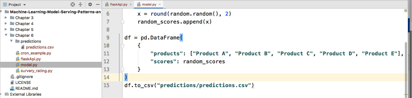
Figure 6.6 – Directory structure of model.py

2. Now, we have to run this model periodically. In order to observe change quickly, we want to run the file every minute. As we have learned, to run a job every minute, the cron expression will be * * * * *. To enter the cron expression, we need to go to the terminal and then type in the crontab –e command, as shown in Figure 6.7.

Figure 6.7 – To edit crontab, the crontab –e command needs to be used

3. After the command, we will see an editor window in which we can enter our command. Enter the command as shown in Figure 6.8.

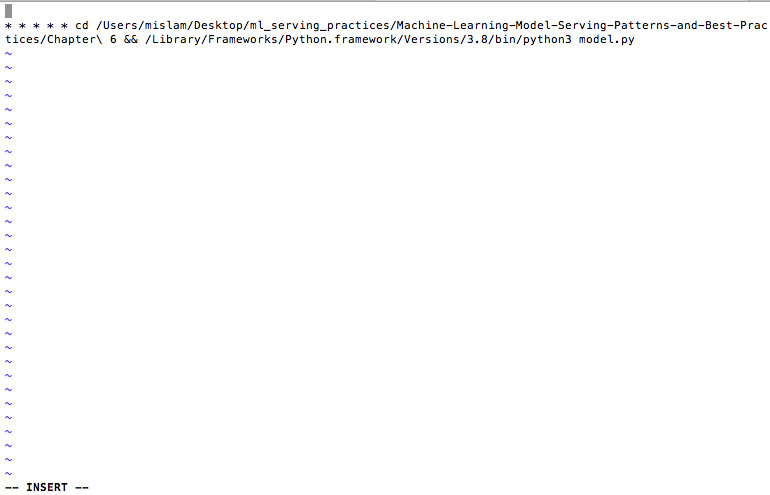
Figure 6.8 – The cron expression added to the crontab for running model.py

The expression is as follows:

* * * * * cd /Users/mislam/Desktop/ml_serving_practices/Machine-Learning-Model-Serving-Patterns-and-Best-Practices/Chapter 6 && /Library/Frameworks/Python.framework/Versions/3.8/bin/python3 model.py

Here, the * * * * * part indicates that the following command will run every minute. Here, we are using two commands. The first command, cd /Users/mislam/Desktop/ml_serving_practices/Machine-Learning-Model-Serving-Patterns-and-Best-Practices/Chapter 6, is used for moving to the Chapter 6 folder, where my Python file is present. The second command, /Library/Frameworks/Python.framework/Versions/3.8/bin/python3 model.py, is used to run the model.py file. Notice that we are using the full path of the python3 binary to run the Python file. You can find the full path to the python3 binary using the which python3 command.

Now, we have scheduled our periodic batch job using a cron expression. Our dummy job will run every minute, but you may schedule jobs with a larger periodic interval.

Storing the predictions in a persistent store

In our model.py program, we are storing the dummy predictions inside a CSV file. If we have a large number of customers, it is ideal to store the predictions in the database.

Let’s check whether our predictions are being written to the CSV file at the expected interval scheduled using the cron job.

If we go inside the predictions folder, we will notice that a CSV file called predictions.csv is being written to every minute.

Figure 6.9 – The CSV file being written to periodically by the batch job

The file and directory structure of the file are shown in Figure 6.9.

Pulling predictions by the server application

When serving the application that uses inferences to the client, the server gets the inferences from the persistence store. The server does not make inference requests directly to the model:

1. To show the server application fetching recommendations from the database, let’s create a basic server using the Flask API as follows:

   import pandas as pd

   from flask import Flask, jsonify

   app = Flask(__name__)

   @app.route""/predict_batc"", methods=''POS''])

   def predict_loading_params():

       df = pd.read_csv""predictions/predictions.cs"")

       predictions = []

       for index, row in df.iterrows():

           product = row''product'']

           score = row''score'']

           predictions.append((product, score))

       predictions.sort(key = lambda a : a[1])

       return jsonify(predictions)

   app.run()

You can see that the server application has one endpoint, "/predict_batch". Once an application hits this endpoint, the server opens a connection to the persistent store. In our case, we open the CSV file to which we are writing predictions in batches.

If we run this application by running the Python program that contains the app.run() code snippet, we will see the following output in the terminal:

* Serving Flask app "flaskApi" (lazy loading)
* Environment: production
   WARNING: This is a development server. Do not use it in a production deployment.
   Use a production WSGI server instead.
* Debug mode: off
* Running on http://127.0.0.1:5000/ (Press CTRL+C to quit)
127.0.0.1 - - [23/Jun/2022 21:41:52] "POST /predict_batch HTTP/1.1" 200 -

2. Now, we can go to Postman to test the endpoint. The Postman interface, after calling this endpoint, will look like Figure 6.10.

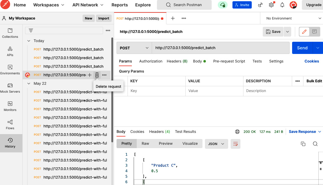
Figure 6.10 – Using Postman to call the http://127.0.0.1:5000/predict_batch API

We have scheduled the batch job to update the CSV file every minute with random scores. The output we get in the first run is the following:

[
["Product C", 0.5 ],
["Product E",0.82],
["Product A",0.89],
["Product B",0.94],
["Product D",0.97]
]

The responses are sorted in increasing order of score.

3. If we make the call again after some time, we will get new predictions. After 2 minutes, we make another call and get the following result:

   [

   ["Product B",0.06],

   ["Product E",0.15],

   ["Product D",0.39],

   ["Product C",0.58],

   ["Product A",0.7]

   ]

The scores and the ranking of the recommendations have also changed.

4. Ideally, the scores will be sorted in reverse order and the recommendation with the highest score will be at the top. To do that, you can add reverse = True to model.py, as follows:

   predictions.sort(key = lambda a : a[1], reverse = True)

The output will now be printed in reverse order. The product with the highest score will come at the beginning of the list as follows:

[
["Product A",0.7],
["Product C",0.58],
["Product D",0.39],
["Product E",0.15],
["Product B",0.06]
]

In this section, we have talked about the techniques in batch model serving by showing an end-to-end dummy example. In this next section, we will discuss some limitations of the batch model serving.

Limitations of batch serving

Batch serving is essential in today’s world of big data. However, it has the following limitations:

• Scheduling the jobs is hard: Scheduling periodic batch jobs is sometimes complicated. As we have seen, during scheduling, the paths expected by the cron expression need to be given carefully. Mostly, cron expressions expect absolute paths. The scheduled jobs may also introduce a single point of failure. If somehow it fails to run on schedule, we might not have the latest inferences, causing a bad customer experience.
• Growth of data will make training slow: If the data grows, the training may gradually take more time. For example, the time needed to train a model with 10 MB of data will not be the same as the time needed to train a model with 10 GB of data. Therefore, we need to take care of this scenario. In most cases, we can discard old data, as it will become stale. Then, the question arises, how old is the data when we consider it stale? We need to identify the answer through empirical evaluation. In some cases, we can say that 1-month-old data is stale and should not be used; in other cases, it can be multiple years.
• Cold start problem: When a new client starts using an application, the user will not have any history that can be used to make recommendations for the user. For example, a new user starts using an e-commerce site. The site will not be able to provide recommendations for the user, as there is no history available for the user and the model will not update until the next scheduled time of training comes. To solve this problem, there are some approaches to provide an initial recommendation. For example, we can look at the user’s age group and other information provided during sign-up to make recommendations from other users with similar personal information.
• Need to maintain a separate database for predictions: We have to store the inference in a separate table or database during batch predictions. This creates additional maintenance overhead. Furthermore, to distinguish between separate batches of inferences, we need to use another column in the prediction table, indicating the batch. Sometimes, we might need to maintain separate tables for storing separate batches of predictions. All these can give rise to technical challenges and technical debts if not handled carefully.
• Monitoring: Monitoring batch serving is also a challenge. As the process runs for a long time, the window of failure is longer. It is also a technical challenge to separate the run between triggered and scheduled batch jobs.

In this section, we have seen some limitations of batch model serving. In the next section, we will draw the summary of the chapter and conclude.

Summary

In this chapter, we have talked about the batch model serving pattern. This is the first pattern that we have categorized based on the serving approaches we discussed in Chapter 2, Introducing Model Serving Patterns. We introduced what batch serving is and looked at the different batch serving patterns based on the batch job triggering strategy and the inference strategy. We explained, with examples, how cron expressions can be used to schedule batch jobs. We discussed some examples where batch serving is essential. Then, we looked at an end-to-end example of batch serving using a dummy model, persistence store, and server.

In the next chapter, we will discuss online serving, which updates the models immediately with new data.

Further reading

We can use the following reading materials to further enhance our understanding:

• To find out more about different metrics in recommender systems, visit https://neptune.ai/blog/recommender-systems-metrics
• To learn more about cron expressions and scheduling cron jobs, visit https://ostechnix.com/a-beginners-guide-to-cron-jobs/