3

Stateless Model Serving

In this chapter, we will talk about stateless model serving, the first pattern-based on serving philosophies. We will first talk about stateless and stateful functions to give you an introduction to these concepts. We will see that stateful functions depend on states within the model and also on the states from the previous calls. Due to these strongly coupled dependencies on states, it is difficult to scale the serving.

When serving is desired, the model is served in a stateless manner so that the model does not depend on previous calls, can be scaled easily, and the output is consistent. However, some machine learning models are by default stateful, and we can attempt to reduce the variance of the server model by using some tricks such as specifying random seeds and using hyperparameters that reduce the variance of the model due to states.

This chapter will give an overview of stateful and stateless functions along with examples. Then we will discuss different kinds of states in machine learning models and how those states are not congenial to scalable and resilient serving. We will also introduce some ideas for reducing the impact of those states.

In this chapter, we will discuss the following topics:

• Understanding stateful and stateless functions
• States in machine learning models

Technical requirements

In this chapter, we will go through some programming examples. To run these programming examples, you need to have a Python IDE setup. You can use Anaconda, PyCharm, or any other IDE you prefer:

• Anaconda download link: https://www.anaconda.com/products/distribution
• PyCharm download link: https://www.jetbrains.com/pycharm/download/

You can see the example code from this chapter and write it manually by yourself, or you can directly clone it from GitHub: https://github.com/PacktPublishing/Machine-Learning-Model-Serving-Patterns-and-Best-Practices.

This GitHub repository contains all the code organized by chapters. The code for Chapter 3 is present here: https://github.com/PacktPublishing/Machine-Learning-Model-Serving-Patterns-and-Best-Practices/tree/main/Chapter%203.

Understanding stateful and stateless functions

Before discussing states in machine learning, we should first understand what stateful functions are and how stateful functions can involve difficulties in serving the function to clients. Therefore, let’s begin by developing a clear understanding of stateful and stateless functions and the differences between them in this section.

Stateless functions

A stateless function does not have any state within the function that can impact the behavior of the function. The output of the function will be the same if the same input is provided. It will also be independent of the platform where the function is stored.

Stateless functions can behave as pure functions. A pure function has the following properties:

• A pure function’s output is identical with identical input. So, y = f(x) is always true. For the same input x, the output is always y. No internal states or variables impact the output and the output is deterministic.
• A pure function will not have any side effects. It will not modify any local variable or state once it is invoked.

For example, consider the following function:

def fun(x):
     return x * x
if __name__ == "__main__":
     print(fun(5)) # Always returns 25

This function is stateless as its output is always the same if the same input is passed. The output from this function neither depends on the states from the function nor makes any modification to any local states. If we look at the advantages of this function, then we will see that the stateless function has the following benefits:

• The output is consistent. So, in a particular instance, all the clients calling the function will get the same result.
• The function can be served through multiple servers to provide consistent service to millions of customers. As this function does not depend on any local state, it can be easily copied to multiple servers and a load balancer can distribute the traffic to different servers. Traffic pointed to different servers has the same consistent results.

We see stateless functions are very convenient from the perspective of serving. However, sometimes we also need to serve stateful functions. In the following section, we will learn about stateful functions, and how can we extract states and convert stateful functions to stateless functions.

Stateful functions

Stateful functions are functions where the output of the function is not solely defined by the input. Stateful functions have some states hidden within the function that have an impact on the output. So, the output is state-dependent and can vary based on the state.

The output of a stateful function depends on the states inside the function and the output will no longer be identical. On the other hand, an invocation of the function can also make modifications to local states. For example, let’s consider the following function:

def fun(x):
     import random
     y = round(10*random.random())
     return x + y
if __name__ == "__main__":
     print(fun(5)) # fun can return any number from 5 to 15 for the same input 5

The preceding function is an example of a stateful function where the internal random state, y, impacts the output of the function.

Why is this problematic?

• The function provides different outputs for the same input. The result does not depend solely on client-passed parameters. So, this function can be a cause of frustration as the clients expect consistent output when they provide the same input unless the business logic of the program expects randomized output, as in some games.
• A function with states cannot be scaled very easily. It might not be very clear from this random state why scaling is a challenge with the states of the model. Think about a system that predicts the temperature and uses one mutable internal state that gets mutated by a caller temperature. This service will be hard to scale to a lot of clients and other client requests will be blocked until the current request is finished. However, there are use cases where stateful serving is good. For example, when enhancing models for language translation, we need previous state data.

Now let’s look at a function where the result of the current function invocation depends on the previous call, such that the current call of the function uses some states from the last call for producing output.

For example, let’s look at the following counter function:

class Counter:
     count = 0
     def __init__(self):
           pass
     def current_count(self):
           Counter.count += 1
           return Counter.count
if __name__=="__main__":
     counter = Counter()
     print(counter.current_count()) # This call prints 1
     print(counter.current_count()) # This call prints 2

In this case, every call to the function depends on the previous call in providing the output.

This dependency causes the following problems:

• Different results based on the order of the calls to the function
• The function cannot be easily served through multiple servers, reducing the scalability options, because the state also needs to be deployed to each server, the servers will easily go out of sync, and the users will keep getting different results from different servers

Extracting states from stateful functions

We have seen two cases where states can cause our program to show inconsistent results and fail to scale easily. The first example has a state within the server that is common to all the functions. The second example shows a scenario where states from previous calls are needed by the current calls.

Now that we know why the preceding functions can be problematic in serving, we need to somehow extract those states or at least reduce the impact of those states.

We can remove the internal state y from the first function and pass the value y from the client side.

The example is shown here:

def fun2(x, y):
     return x + y
if __name__ == "__main__":
     import random
     y = round(10*random.random())
     print(fun2(5, y)) # fun2 will return same output for 5 and same value of y

We see the function has been modified from stateful to stateless by extracting the state y and taking the responsibility of passing the state from the client. This kind of conversion adds an extra burden on the client. Now, we notice fun2 adds the following advantages:

• The output is now consistent. If the client passes the same input data, it will always return the same output data
• The function can be parallelly deployed to many servers and can serve billions of clients without dropping performance

However, with fun2, the client has to take responsibility for managing states and passing them to the function.

In web API calls, the client needs to pass all the necessary states with every call. The server does not store anything, indicating each of the calls is independent of one another. That is why these APIs are called Representational State Transfer (REST) APIs. So, any function that needs to be scaled and resilient needs to be stateless as much as can be.

Similarly, for the second function, we can pass the state count with every call. So, a particular client will always get the same response based on the input the client passes:

def current_count(prev_count):
     return prev_count + 1
if __name__=="__main__":
     counter = Counter()
     print(counter.current_count(1)) 

The call to current_count() now takes the previous state as shown in the preceding code and removes the dependency on the previous call. So, this call now returns the same output based on the identical input. This can now be scaled easily. The servers will not go out of sync and the users will also get consistent output based on the input they provide.

The preceding examples show some simple stateful functions and how they can be converted to stateless, but when might it be useful to have stateful functions?

Using stateful functions

Stateful does not always mean bad. Sometimes, you need to have some states preserved by the function. For instance, you may be familiar with the singleton pattern, which is a famous pattern used widely in software and serving applications. Note that a singleton is a global variable and needs to be used carefully to avoid side effects. For example, privileges for database connectivity for different kinds of users might be different, but if the connection object does not update for different kinds of users, that might cause serious problems. The singleton pattern creates and stores the instance of an object internally as a state and returns the same object in subsequent calls. If the object is already initialized, then it does not re-create the object and returns the already available object. To understand this in practice, let’s look at the following code example of the singleton pattern:

class DbConnection(object):
     def __new__(cls):
           if not hasattr(cls, 'instance'):
                 print("Creating database connection")
                 cls.instance = super(DbConnection, cls).__new__(cls)
                 return cls.instance
           else:
                 print("Connection is already established!")
                 return cls.instance
if __name__=="__main__":
     con1 = DbConnection() 
     con2 = DbConnection()
     con3 = DbConnection()

This code shows the following output in the console:

Creating database connection
Connection is already established!
Connection is already established!

From the output, we see that the connection instance is created only once and, based on the state of the connection that is tracked by the function as the internal state, we get a different output. Though, in this case, we get only two different outputs, multiple desirable outputs may be seen based on the state of the function.

Stateful functions can be used in many cases. Some of those use cases may be the following:

• In distributed computing, when we need to keep track of different nodes in the cluster, and to join the results correctly as in MapReduce, we need to store the states identifying the nodes and targets during joining.
• In a database, we need to store the indices of the table as states so that we can quickly fetch the data by using the indices.
• During online shopping, the server needs to store the shopping cart information for the user.
• Recommendation engines need to store the customer’s previous activities to recommend effective suggestions.

Therefore, stateful functions are not always bad. However, these states must be managed carefully to reduce the side effects of scalable serving. For example, a big data cluster will keep the metadata about all the nodes in some central or master nodes so that other child nodes can scale well. Similarly, we need to be careful in serving stateful applications and need to reduce the impact of serving states as much as possible.

In some models, such as sequence models, stateful serving is the option to choose. These models usually take multiple sequential requests and the inference of one request depends on the previous inference. In this way, keeping the state of the previous stage is required. To learn more about different stateful models, please follow this link: https://github.com/triton-inference-server/server/blob/main/docs/user_guide/architecture.md#stateful-models.

In this section, we have discussed stateful functions, and the challenges involved with stateful functions in model serving. We have also seen simple examples of how a stateful function can be converted to stateless. In the next section, we will see some of the common sources of states in machine learning.

States in machine learning models

A machine learning model, at a high level, can be seen as a mathematical function, y = f(x). We provide the input data and train the model. However, the model can perform differently based on the following things:

• Input data: The quality of input data, features extracted from the input data, volume of the input data, and so on
• Hyperparameters: Learning rate, randomness to avoid bias and overfitting, cost functions, and many more

As these things impact the performance of the model, if they are used as states during serving, scaling can be a challenge, as well as consistency in response to customers.

Now we will look at some cases of how a machine learning model can have states.

Using input data as states

A machine learning algorithm can be designed in such a way that the data used during training is used as states for the model. This can be done in the following two ways:

• Some artificial data is generated to enhance the performance of the model. It is done within the serving of the application and this data can be used for training whenever a retrain action is triggered.
• Input data is used in combination with the features in the feature store (a feature store is a database where we keep the pre-computed features)  to update the model in later iterations for online serving. In that case, input from one request is used to alter the model’s performance. So, each request is important to the overall model performance.

In both of these cases, the model is dependent on the local states. If we try to scale the model to a second server, we will face difficulty, as these local states need to have consistent values in all the servers. This is almost impossible. We would violate the CAP principle.

The CAP principle is a well-known principle in computer science where C stands for consistency, A stands for availability, and P stands for partition tolerance. This principle states that in a distributed system we can guarantee only two of these three properties. To know more about this principle please follow the link here, https://en.wikipedia.org/wiki/CAP_theorem.

We can clearly see that if we try to create a replica of the model on multiple servers, we will have obvious issues with consistency. One aspect of the consistency principle is that all the servers should return the same response at the same time from the same request.

However, in this case, we will violate the consistency principle in the following ways:

• Generated data usually involves a stochastic process. So, the data in different nodes will be different, causing the problem of having different models.
• Let’s assume a hypothetical scenario, where there is a separate copy of training data in all the nodes that is used to update the models in respective servers. So, there are multiple sources of truth. If the data in one node is modified for some reason, then that node will have a different ground truth for training the model.
• If the data is being read from a streaming source, then the data reading latency in different nodes may be different. So, the data in different nodes will very often fall out of sync. This violates the consistency principle.
• The training convergence in different nodes may take different lengths of time, causing the nodes to go out of sync. This violates the consistency principle.

There can be many other problems if we use the training data as states in a serving model. We might try to solve some of the problems by storing the data files in a central node. This is a good start to resolve some challenges. However, still we are burdened with the following problems:

• The latency of the data being read from that central node by the serving nodes might be different, violating consistency and availability.
• The data communication overhead is high. Packets may be lost, leading to different data at different nodes. If the data is big, then it becomes more challenging. One solution might be to fetch a single batch of data in each call. However, we can clearly see the problem. Thousands of network communication calls are going on with a high payload, incurring costs on our end. Also, as the communications will have different latencies and could also be lost, we are still not solving the fundamental violations of consistency and availability.

We see that using training parameters as state can turn into a big headache during model serving. Other than the problems mentioned previously, there can be many other problems and side effects. Obviously, the business impact of serving a model with these states will be negative; nobody wants unhappy clients. We should get rid of these states before serving the model.

In this section, we have seen how using training data as states can badly impact serving. In the next section, we will look at random states in a machine learning model.

Random states in model training

Machine learning models are stochastic in nature. So, during the training of the model with the same data, we can have different models with different times giving different predictions.

For example, let’s consider the following RandomForestRegressor model:

from sklearn.datasets import make_regression
X, y = make_regression(n_features=2, random_state=0, shuffle=False, n_samples=100)
model = RandomForestRegressor(max_depth=2)
model.fit(X, y)
print(model.predict([[0, 0]]))

The output of the model for five runs is the following:

[35.67162367]
[31.09473468]
[32.65963333]
[32.29529916]
[28.72626675]

We see that the outputs are different at different times even though the same data is being used for training. The output ranges from [28.72626675] to [35.67162367] in just five different runs.

If we look at the tree of the model that is trained in two different runs, we will understand how complex the model is. There are 100 different trees learning in the preceding model.

We can see that number with the following code:

print("Total estimators", len(model.estimators_))

It will give the following output:

Total estimators 100

Note

We can also specify the number of estimators during training. We have just used the default parameters to avoid complexity and show how the model can behave differently by selecting the parameters themselves.

To understand how different models can vary, let’s visualize only the first tree of the random forest algorithm in two different runs.

Figure 3.1 shows the visualization of the first tree in the first run.

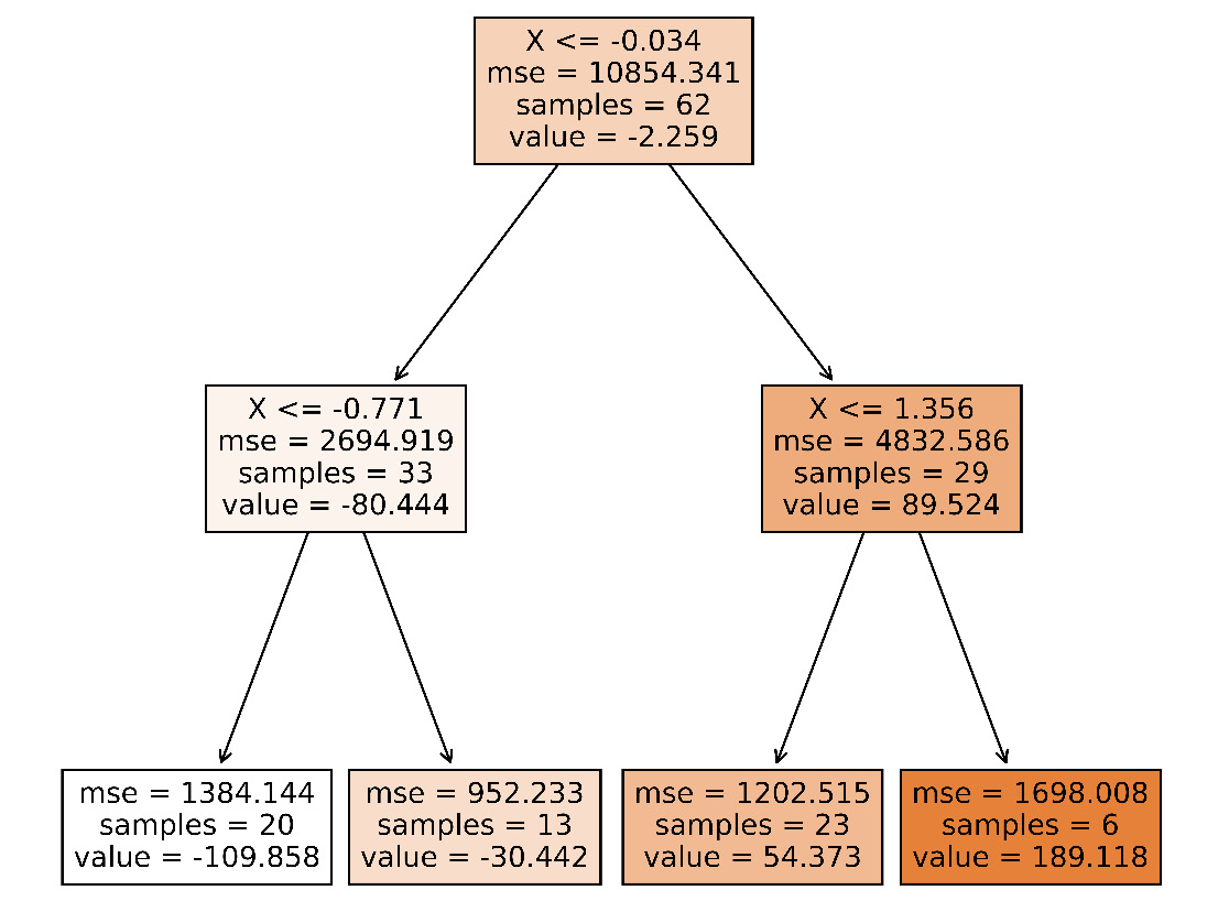
Figure 3.1 – The first decision tree of the random forest learnt in the first run

Note

Mean Square Error (MSE), shown in Figure 3.1, is the average of squares of the differences between predicted and actual values.

For example, let’s say for five instances, x1, x2, x3, x4, x5, the actual labels are y1, y2, y3, y4, y5 and the predicted values from the model are y’1, y’2, y’3, y’4, y’5.

Therefore, the MSE in this case is [(y1 - y’1)^2 + (y2 - y’2)^2 + (y3 - y’3)^2 + (y4 - y’4)^2 + (y5 - y’5)^2]/5.

To read more about MSE, please follow the link: https://statisticsbyjim.com/regression/mean-squared-error-mse/.

Figure 3.2 shows the visualization of the first tree in the second run.

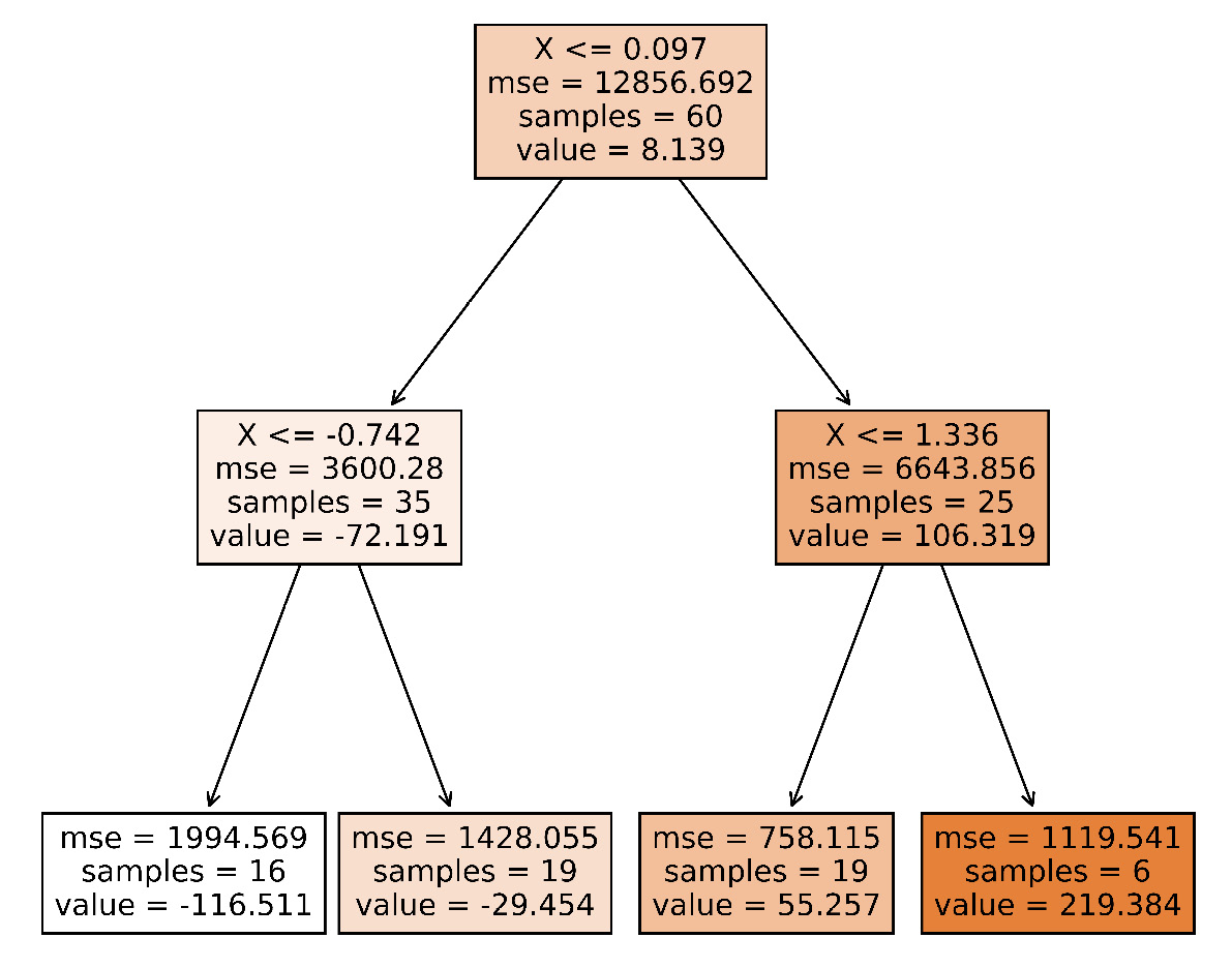
Figure 3.2 – The first decision tree of the random forest in the second run

We have used 100 samples to generate our trained model. If we just look at the root node of both the decision trees in Figure 3.1 and Figure 3.2, we will see many clear differences. The first node in Figure 3.1 got 62 samples out of 100 after training. The other 38 went to other decision trees that we have not shown. And we see these 62 got further split into two nodes with 33 and 29 samples. The node with 33 samples got further split into two different nodes with 20 and 13 samples. These leaf nodes are also called decision nodes, which return the decision.

Let’s see the difference in the two decision trees in the following table only for the first node:

Figure 3.3 – Differences between metrics on the first decision tree of the random forests trained with the same data

From the table in Figure 3.3, we see the differences are significant. The same data point might have a totally different decision path only in the first decision tree.

The decision path is the path followed by the input sample to reach the decision node. For example, if we wanted to predict the output for the input data Xi = 1.0 using the decision tree in Figure 3.2, we would follow this path:

1. Start at the node with condition X <= 0.097.
2. Move to the right children node with the condition X <= 1.336.
3. As Xi = 1.0 satisfies the condition X <= 1.336, move to the left child with the value = 55.257.

Decision paths

To learn more about decision paths, you can follow this link: https://scikit-learn.org/stable/auto_examples/tree/plot_unveil_tree_structure.html#decision-path.

And if we look at the textual representation of the first decision, at a particular node, we will understand how many states the model is storing just for a single node:

DecisionTreeRegressor(ccp_alpha=0.0, criterion='mse', max_depth=2,max_features='auto', max_leaf_nodes=None, min_impurity_decrease=0.0, min_impurity_split=None, min_samples_leaf=1, min_samples_split=2, min_weight_fraction_leaf=0.0, presort='deprecated',random_state=554039182, splitter='best')

All these states can have more or less of an impact on the behavior of the model. If we use some kind of parameter selection algorithm, then the selected parameters and their values might also be different in different runs.

In this section, we have seen that random states within a model can yield inconsistency in responses, causing a bad customer experience. The prediction path might also be different at different times for the same data with the presence of these random states within the model.

In the next section, we will look at the weights and bias states of models, especially deep learning models.

Using model weights as model states

Deep learning models usually have a lot of weights and biases across different layers.

A deep learning model has three kinds of layers: an input layer, hidden layers, and an output layer. There can be one or more hidden layers. Based on the number of hidden layers, a neural network is sometimes referred to as a shallow neural network or a deep neural network.

To understand the weights and biases in neural networks, we will use the example shown on the official TensorFlow website: https://www.tensorflow.org/datasets/keras_example.

We can make some minor changes to the model, as follows:

model = tf.keras.models.Sequential([
  tf.keras.layers.Flatten(input_shape=(28, 28)),
  tf.keras.layers.Dense(8, activation='relu'),
  tf.keras.layers.Dropout(0.5),
  tf.keras.layers.Dense(10, activation='softmax')
])

The modified code can be found in the GitHub repository for this book, under the folder for Chapter 3. We have changed the hidden layer dimension from 128 to 8 to make it easier to read the states.

Note

Our goal is not to build an efficient machine learning model in any of the chapters. Our goal, rather, is to educate in serving the model, which is the next step after building the model. For further understanding of the importance of the model serving step in the machine learning development life cycle, please refer to Chapter 1. Sometimes, we will use some parameters just to ensure better visibility and readability of the states.

We have also changed the epochs from 6 to 3 and added an additional layer, tf.keras.layers.Dropout(0.5), to see the impact of states on different runs. This is an important layer in deep learning models for regularizing and avoiding overfitting.

If we print the model summary after training, using the code model.summary(), we will be able to see a summary of the number of parameters or states at different layers. For the example, we extracted data from the official TensorFlow website and modified it a little to see the following output:

_________________________________________________________________
Layer (type)                        Output Shape                    Param #   
=================================================================
flatten (Flatten)                 (None, 784)                     0            
_________________________________________________________________
dense (Dense)                       (None, 8)                        6280        
_________________________________________________________________
dropout (Dropout)                 (None, 8)                        0            
_________________________________________________________________
dense_1 (Dense)                    (None, 10)                       90           
=================================================================
Total params: 6,370
Trainable params: 6,370
Non-trainable params: 0

We see there are 4 layers and in total there are 6,370 parameters. The model we used is very simple and we have also reduced the model size to ensure we can observe the parameters better. Out of those layers, there are parameters only on the two dense layers. The Flatten and the Dropout layers do not have any parameters or states.

Now we can do some mathematics to understand how the number of parameters in the first dense layer is 6,280 and in the second dense layer is 90.

Each of the mnist images we are using is of size (28, 28). So, if we vectorize this (28, 28) matrix, we get a vector of size 28*28 = 784.

Now, each of these 784 pixels will densely connect with the following dense layer, forming connections of size (784, 8) as the dense layer has a dimension of 8. So, in total, there are 784*8=6,278 connections from the input layer to the dense layer. And the first dense layer has 8 nodes. Each node has a bias value adding 8 more parameters for 8 nodes in this dense layer. So, in total, there are 6,278 + 8 = 6,280 parameters for the first dense layer.

In the second dense layer, there are 90 parameters. Let’s compute where these 90 parameters come from.

The first dense layer connects to the second dense layer, the output layer. Each of the 8 nodes from the first dense layer connects with each of the 10 nodes in the second dense layer. So, we get a total of 8*10 = 80 connections. Each of these 80 connections has a weight. And each of the 10 nodes in the output dense layer has a bias. So, in total 80+10 = 90 parameters for the last dense layer.

Let’s try to see the value of these states. We add the following code after training the model to see the weights and bias of the dense layers after training:

W = model.variables
print(len(W))
print("Weights for input Layer to hidden layer")
print(W[0])
print("Shape of weights for input layer to hidden layer", W[0].shape)
print("Bias of the Hidden Layer")
print(W[1])
print("Shape of the bias of the hidden layer", W[1].shape)
print("Weights of the hidden to output layer")
print(W[2])
print("Shape of the weights of the hidden to output layer", W[2].shape)
print("Bias of the output layer")
print(W[3])
print("Shape of the bias of the output layer", W[3].shape)

We will be able to see the weights and biases, like the following:

Weights from the input layer to the hidden layer

Let’s look at the output from the following code snippet:

print(W[0])
print("Shape of weights for input layer to hidden layer", W[0].shape) 

We will see the weights from the input layer to the hidden layer, as follows, along with the information on the dimension of the weights:

<tf.Variable 'dense/kernel:0' shape=(784, 8) dtype=float32, numpy= array([[-0.03122425,  0.08399606,  0.05510005, ...,  0.03683829, -0.08382633,  0.03250936],

Here is the truncated output:

[-0.08059934,  0.07114483, -0.05455323, ..., -0.01873366,  -0.08493239, -0.06046978]], dtype=float32)>

The shape of the weights from the input layer to the hidden layer is (784, 8).

We see that the size of the matrix of weights in between the input layer and the hidden layer is (784, 8). So, in total, there are at least 784*8 different states that impact the data that proceed from the input layer to the hidden layer during prediction. I am saying at least because there are some other states that also impact the manipulation of data, such as bias.

Bias of the hidden layer

We can now observe the output from this part of the above code snippet:

print(W[1])
print("Shape of the bias of the hidden layer", W[1].shape)

We will print the biases and the shape of the biases of the hidden layer, as follows:

<tf.Variable 'dense/bias:0' shape=(8,) dtype=float32, numpy=
array([-0.04289399, -0.14067535,  0.28432855,  0.17275624,  0.16765627, 0.15334193,  0.14531633, -0.17754607], dtype=float32)>

The shape of the bias of the hidden layer is (8,).

For each of the nodes in the hidden layer, there is a bias term. This bias term impacts the data that flows from a node. For example, if the bias value for a particular node is —1 and the data that comes from the input layer to this node is 1, then the data that will flow out from this node is –1 + 1 = 0. That means this node will not have any contribution in the following layer.

Weights from the hidden to the output layer

To get the weights from the hidden layer to the output layer, we use the following code snippet:

print(W[2])
print("Shape of the weights of the hidden to output layer", W[2].shape)

This produces the weights and the shape as follows:

<tf.Variable 'dense_1/kernel:0' shape=(8, 10) dtype=float32, numpy=
array([[-0.5102042 , -0.29024327,  0.73903835,  0.06289692, -0.2546525 ,

Here’s the truncated output:

0.462961, -0.7462656 , -1.1991613, 0.40228426,0.14731914]], dtype=float32)>

The shape of the weights matrix from the hidden layer to the output layer is (8,10). Therefore, there are 8*10 = 80 state values that impact the data that will flow to the output layer.

Bias of the output layer

We can get the biases and the shape of the biases of the output layer with the following code snippet:

print(W[3])
print("Shape of the bias of the output layer", W[3].shape)

The output we get is the following:

<tf.Variable 'dense_1/bias:0' shape=(10,) dtype=float32, numpy= array([ 0.02194504,  0.48662037, -0.3252962 ,       -0.07106664, -0.03191056, 0.29797274, -0.08240528,         -0.35948208,  0.4130473 , -0.41163027],dtype=float32)>

The shape of the bias of the output layer is (10,).

For each of the 10 output nodes, we have a bias node.

From the states in the preceding code, we can see that in a deep learning model, there can be numerous states that impact the inference from the model. If these states are not carefully managed, they can create an impediment to scalable and resilient serving. To understand why states can cause an impediment to serving, let’s look at the following example.

The weights and bias are updated via training. We will see that these outputs and biases are different if we run the training again with the same data. For example, let’s look at the bias output of the dense_1 layer in a different run to see the difference:

array([ 0.0370706 , -0.35546538, -0.4211915 ,  0.49760145, -0.12625118, 0.21710081, -0.28547847,  0.3222543 ,         -0.26602563,  0.27582088], dtype=float32)>

The shape of the bias of the output layer is (10,).

We see each of the bias values for the 10 nodes is different for the two consecutive runs with the same data.

Figure 3.4 – Differences of biases in the last dense layer in two consecutive runs

From the table in Figure 3.4, we see that the value of weights and bias weights vary a lot in two consecutive runs. While training deep neural networks random initialization of the weights and biases is needed for the successful convergence of the model. However, this creates an additional burden for us while serving the model. These states have an impact on the model output. So, the model that is trained does not behave as a pure function and can have different values, depending on the values of these states.

We can save the model to a directory called saved_model using the following command:

model.save('saved_model')

After the model is saved, we will see a structure like the following:

saved_model
     -> assets
     -> variables
-> variables.data-00000-of-00001
-> variables.index
     -> saved_model.pb

We notice the model structure is located in the saved_model.pb file and all other states are stored in the assets and variables folder. We can also save the model as JSON by converting the model to JSON using the following command:

 json = model.to_json()

We can then view the model structure as follows in Figure 3.5:

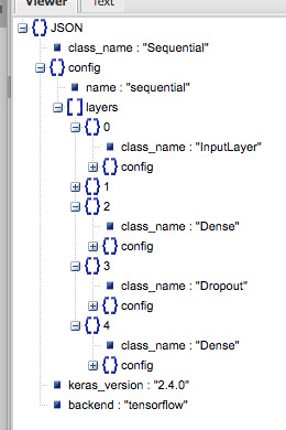
Figure 3.5 – JSON view of the JSON representation of the model

This view is generated from the public tool at http://jsonviewer.stack.hu/. You need to paste the JSON there and it will create a view like the one in Figure 3.5.

With all these states, this model is heavily dependent on the local environment.

This stateful nature of the model due to the states from weights and biases will create the following problems in model serving:

• If we serve a different copy of the model using a different pipeline, then the response from the models will be different even though the models are following the same algorithm and the same input data distribution. So, a client making a call to the prediction API might get two different responses at two different times due to a load balancer forwarding the requests at different times based on traffic loads.
• Scaling the serving is difficult as the models might go out of sync for reasons related to retraining, transfer learning, online learning, and many other reasons.
• For continuous evaluation, the models on different servers will need to update at different times and will quickly go out of sync. For example, let’s say we monitor the performance of three copies of the same model on three servers: S1, S2, and S3. We use the same metric that we used during training to evaluate the performance of the models. Let’s say the performance of the model on S1 falls below the threshold value of the accepted error rate (which depends on the problem and business goal) at time T1. In this case, we need to do some hard work. We have to retrain the model and copy the reatried model to all the single servers before the responses from all the servers can be in sync. If we just retrain the model on server S1, then the model will be out of sync with the other ones.
• During online training, it is hard to train the models continuously, as whenever new data comes in, we need to retrain and the models on all the servers will become out of sync very quickly.

In this section, we have seen how we can compute the number of parameters in a basic densely connected neural network. In the following section, we will see the number of parameters in a Recurrent Neural Network (RNN).

States in the RNN model

To demonstrate the weights and parameters in the RNN model, let’s use the example from the official TensorFlow site: https://www.tensorflow.org/guide/keras/rnn.

The example code is also present in the GitHub repository of this book, under the Chapter 3 folder.

Let’s first build the model using the layers shown here:

model = Sequential()
model.add(Embedding(input_dim=1000, output_dim=64))
model.add(LSTM(128))
model.add(Dense(10))

We will be able to see the number of parameters in different layers using model.summary(). We will get the following model summary after running the model.summary() statement:

Model: "sequential"
_________________________________________________________________
Layer (type)                        Output Shape                    Param #   
=================================================================
embedding (Embedding)           (None, None, 64)              64000      
_________________________________________________________________
lstm (LSTM)                          (None, 128)                     98816      
_________________________________________________________________
dense (Dense)                       (None, 10)                       1290        
=================================================================
Total params: 164,106
Trainable params: 164,106
Non-trainable params: 0

Now, let’s try to understand the states in each of the layers. The number of parameters in the Embedding layer is found by multiplying the input dimension by the output dimension. That means each of the input edge weights connects to each of the output edge weights in a cross-multiplication manner. So, we get the total parameters in this layer as 1000*64 = 64000.

In the LSTM layer, the number of parameters is 98,816. To compute the number of parameters in the LSTM layer, we need to take the following states:

1. Compute the number of edges going from the input to different units for each of the gates and the number of bias terms for each of the units in the LSTM gate. In LSTM, there are four gates. So, for four gates, we get 4*(input_dim*units+ units) = 4*(64*128+128) = 33,280.
2. Compute the number of weights that are coming from feedback edges for each output node of the output layer. We know the output dimensions at time T are fed back to each of the units in time T + 1 for recurrency. So, the number of parameters for this recurrency for all four gates is 4*units*units = 4*128*128 = 65, 536.
3. Add the numbers from step 1 and step 2 to get the total number of parameters in the LSTM layer. So, the parameter total for this model is 33, 280 + 65, 536 = 98, 816.

We have already shown how to compute the number of parameters in the Dense layer in the previous section. Using the same approach in this Dense layer, the number of parameters is = 128*10 + 10 = 1,290.

In the last two sections, we have seen that a deep learning model can have millions of parameters as states within the saved model. These states make the model a non-pure function and the response is heavily dependent on the states, which violates a number of fundamental principles in serving, carrying the risk of an unhappy client experience. In the next section, we will look at the parameters or states in a regression model and understand their impact on serving.

States in a regression model

States in a regression model mainly come from the regression parameters. The regression model has two main kinds of parameters. The structure of a regression equation is y = ax + b. Here, the two parameters are a and b:

• Intercept: Parameter b in the previous equation is called the intercept. To understand what it implies, let’s say x = 0. So, we get y = b. This is a line parallel to the x axis and intercepts the y axis at point (0, b).
• Slope: The a parameter is known as the slope. It can be defined as the rate of change of y or the amount of change of y if x changes by 1. Sometimes this is also known as the coefficient. For each of the input features, there will be a separate coefficient in a simple linear regression model.

To demo the parameters in a simple linear regression model, let us take the following code snippet from https://scikit-learn.org/stable/modules/generated/sklearn.linear_model.LinearRegression.html:

import numpy as np
from sklearn.linear_model import LinearRegression
X = np.array([[1, 1], [1, 2], [2, 2], [2, 3]])
y = np.dot(X, np.array([1, 2])) + 3
reg = LinearRegression().fit(X, y)
reg.score(X, y)
print(reg.coef_)
print(reg.intercept_)
print(reg.predict(np.array([[3, 5]])))

Here, the output we get from the three print statements is as follows:

[1. 2.]
3.0000000000000018
[16.]

We can see there are two slopes/coefficients, 1 and 2, for 2 input features, x1 and x2, in input data X. For example, in the first input instance in X, the value of x1 = 1 and the value of x2 = 1. And here, the intercept is 3.0000000000000018~ 3.0.

So, we can write the regression equation as follows:

In the third print statement, print (reg.preditc(np.array([3, 5]))), we are doing a prediction for [3, 5] and we have seen the output of 16 as shown in the preceding output, [16.].

Now, let’s compute the prediction using the regression formula:

We got the same result. From this, we understand these states have a direct impact on the result that we get. Therefore, these states can cause difficulties during serving if not managed properly. For example, if we serve a regression model in different nodes in different regions, those servers can go out of sync if the training data is not updated simultaneously on all servers. This will create difficulties in maintenance and the serving or deployment pipeline can become unstable due to the heavy maintenance overhead.

States in a decision tree model

To understand the states in a decision tree model, let’s consider the following code snippet:

from sklearn import tree
import matplotlib.pyplot as plt
X = [[0, 0, 2], [1, 1, 3], [3, 1, 3]]
Y = [0, 1, 2]
clf = tree.DecisionTreeClassifier()
clf = clf.fit(X, Y)
print(clf.predict([[3, 1, 6]]))
print(clf.predict([[1, 1, 6]]))
print(clf.decision_path([[3, 1, 6], [1, 1, 6]]))
tree.plot_tree(clf)
plt.show()

This is a very basic model to show the states that can affect decision-making. We can see the output tree in Figure 3.6.

Figure 3.6 – Graphical representation of the decision tree

Gini

In Figure 3.6, we can see a metric called gini. It is known as the gini index or the gini coefficient. Gini impurity is the default criteria used by a decision tree in scikit-learn to measure the quality of the split of data points to children. If the gini index value is 0, then the samples are assumed to have perfect equality and no further splitting is needed.

That’s why we see in all the child nodes in Figure 3.6 that the gini index is 0. A gini index of 1.0 indicates maximum impurity.

Therefore, as the decision tree evolves from the root node, the gini index decreases, indicating the samples are getting more and more homogeneous.

To read more about the gini index and the formula used to compute the gini index, you can follow this link: https://en.wikipedia.org/wiki/Gini_coefficient.

Now let’s try to understand how states impact making decisions. During decision-making, the states that will be used are the following:

• Conditional states in each of the non-leaf nodes, such as X[0] <= 0.5
• The value state in the leaf nodes or decision nodes

The state value represents the target label for this node. For example, a leaf node with the value [0, 1, 0] means any instance that comes to this node will be labeled as Y[1] as position 1 is set in the value. Please note that the value has only three elements as our input used during training is of size 3. Now let’s try to understand how we can predict X1= [3, 1, 6] using the decision tree shown in Figure 3.6:

1. At the root node, we check X[0] <= 0.5. In other words, 3 <= 0.5. As this condition is false, we go to the right child node.
2. At the right child node, the condition is X[0] <= 2.0, or 3 <= 2.0. This condition is false. So, we reach the rightmost leaf node from here. Here, we see the value is [0, 0, 1].
3. We return the prediction as Y[2] = 2.

We notice that we get the same output from the statement print(clf.predict([[3, 1, 6]])).

If we follow the same steps for the input X2 = [1, 1, 6], we will end up at the leaf node with the value [0, 1, 0], yielding the prediction Y[1] = 1. This is the same result we get from the statement print(clf.predict([[1, 1, 6]])).

We can path followed by the input in the decision tree to make a decision using the decision paths from the statement print(clf.decision_path([[3, 1, 6], [1, 1, 6]])). The output of this statement is the following:

  (0, 0)  1
  (0, 2)  1
  (0, 4)  1
  (1, 0)  1
  (1, 2)  1
  (1, 3)  1

We see a sequence of tuples (i, j) where i is the sample number in the data passed to the function decision_path(X). For example, in our input [[3, 1, 6], [1, 1, 6]], we have two samples. The sample at index 0 is [3, 1, 6] and the sample at index 1 is [1, 1, 6]. And the term j indicates the node number in the array representation of the tree. During the array representation of a binary tree, the root node is placed at index 0, the left child is placed at index 2*0 + 1 = 1, and the right child is placed at index 2*0 + 2=2. This process continues recursively. The general formula is the left child of a node at index n is placed at index 2*n + 1 and the right child is placed at index 2*n+2.

Other than these two states, conditional expression and value, other states will have an impact on the training time. If those states are different, the models will be different.

In this section, we have seen the states that impact the inference in a decision tree. If we rerun the code shown previously, we will get a different decision tree from Figure 3.6. Therefore, these models are very sensitive to states.

Serving this model will encounter similar problems to those listed in earlier sections.

In the last few sections, we have explored states in some basic DNN models, RNN models, ensemble models (the random forest regression model), the linear regression model, and decision tree models. We can use the same strategy to understand different states in other models and to understand how the states impact inference and serving. This understanding of states is a critical step before we can decouple states to ensure scalability and resiliency in model serving.

In the next section, we will discuss how can we remove or reduce the impact of these states during serving.

Mitigating the impact of states from the ML model

We learned about states in some ML models in the last section and have seen how serving can be inefficient in the presence of these states. In this section, we will look at some ideas we can use to minimize the impact of states and ensure resilient serving.

Using a fixed random seed during training

Some models use random seeds during training that are used to initialize the values for some of the states:

1. As an example, let us take the random forest model shown before and add a fixed random state, random_state=0, to the model as follows:

   model = RandomForestRegressor(max_depth=2, n_estimators=10, random_state=0)

Now, the model will give the same result for the prediction print(model.predict([[0, 0]])).

2. We run the model five times and we get the same output every time:

   [38.23613716]

   [38.23613716]

   [38.23613716]

   [38.23613716]

   [38.23613716]

If we use the same data for training, then we will have the same model each time we train unless we don’t change the value of random_state.

However, if we change the data, then the models will be different.

Moving the states to a separate location

After training the model, we can move the states to a separate location. All the models, before making a prediction, will fetch the states from that location. That separate location can be a master node in the distributed cluster or content store. Now the inference flow will look something like what’s shown in Figure 3.7.

Figure 3.7 – Inference steps with states stored in a separate location

Once the model receives a prediction request, it will fetch the required model states from the state store. The states will then be applied to the model and predictions can be made from the model.

This approach has the following drawbacks:

• The additional calls to the state storage will add latency. We have to then consider the trade-off of updating the model states from the state storage periodically instead of for every client call.
• The size of the parameters can be big. So, we need to identify which parameters are safe to stay in the model without causing any side effects and decouple only the parameters that are most important and mutable.

This state storage will be common to all servers and the server can stay in sync by getting the parameters from the state storage from time to time.

If at a time instance, t, the state is updated, all the servers will be notified and they will take the new states from the state storage. We can avoid copying the model to the servers unless the model structure is changed and load the states only from the central store location.

To demonstrate this, let’s take a very simple example using the decision tree we had before, and perform basic serving using the Flask API:

1. First of all, let’s save the model and the model params separately using the following code:

   from sklearn import tree

   import pickle

   X = [[0, 0, 2], [1, 1, 3], [3, 1, 3]]

   Y = [0, 1, 2]

   model = tree.DecisionTreeClassifier()

   model.fit(X, Y)

   with open("models/dt.pkl", "wb") as file:

        pickle.dump(model, file)

   print(model.predict([[1, 1, 6]]))

   params = model.__dict__

   with open("state_store/dt_params.pkl", "wb") as param_file:

        pickle.dump( params, param_file )
2. Next, we store the model in the models folder in a file called dt.pkl. We separately store the model parameters in the state_store folder in the dt_params.pkl file. We are training here with the same data as before:

   X = [[0, 0, 2], [1, 1, 3], [3, 1, 3]]

   Y = [0, 1, 2]

And we get the output of [1] from the line print(model.predict([[1, 1, 6]])).

Now let’s serve this model using the Flask API.

3. We will use the following code snippet to create serving endpoints using Flask. In this code sample, we create two REST API endpoints using flask for serving the model. One endpoint loads the model and parameters separately and the other endpoint loads the full model with parameters embedded as states of the model. We load the model using the pickle library and get the prediction of the data passed by the user. We explicitly indicate the type of the model after loading in the snippet model: tree.DecisionTreeClassifier as, by default, at the static compile time, the type is not resolved and we will not get autosuggestions for methods and attributes of the model during development. For predicting, we need to convert the JSON data to a numpy array using json.loads(request.data) as the predict method accepts numpy ndarray and returns numpy ndarray as a response. To encode numpy ndarray as JSON during the response, we create a custom encoder, NumpyEncoder. Without this, we will get an error as JSON, by default, does not know how to encode numpy ndarray as JSON:

   import json

   import pickle

   from sklearn import tree

   import numpy as np

   from flask import Flask, jsonify, request

   class NumpyEncoder(json.JSONEncoder):

        def default(self, obj):

              if isinstance(obj, np.ndarray):

                    return obj.tolist()

              return json.JSONEncoder.default(self, obj)

   app = Flask(__name__)

   @app.route("/predict-with-params", methods=['POST'])

   def predict_loading_params():

        with open("dt.pkl", "rb") as file:

              model: tree.DecisionTreeClassifier = pickle.load(file)

              # Loading params from param store

              param_file = open("../state_store/dt_params.pkl", "rb")

              params = pickle.load(param_file)

              print(params)

              model.__dict__ = params

              X = json.loads(request.data)

              print(X)

              response = model.predict(X)

              return json.dumps(response, cls=NumpyEncoder)

   @app.route("/predict-with-full-model", methods=['POST'])

   def predict_with_full_model():

        with open("dt.pkl", "rb") as file:

              model: tree.DecisionTreeClassifier = pickle.load(file)

              X = json.loads(request.data)

              print(X)

              response = model.predict(X)

              return json.dumps(response, cls=NumpyEncoder)

   app.run()

We load the model every time in the preceding dummy example. In reality, we might use a singleton service to return the model to avoid expensive I/O operations for each call. After running the application, we will see output like the following:

* Serving Flask app "flaskApi" (lazy loading)
* Environment: production
   WARNING: This is a development server. Do not use it in a production deployment.
   Use a production WSGI server instead.
* Debug mode: off
* Running on http://127.0.0.1:5000/ (Press CTRL+C to quit)

Please note the URL http://127.0.0.1:5000/ as we will be using it in Postman. Postman is a REST API client.  

We have two endpoints: /predict-with-full-model, which will do the prediction using the full model, and the other endpoint is /predict-with-params, which will not use the static model – it will fetch the parameters from the param store and fill the model with new parameters. We have moved the dt.pkl file to the serving folder. Now let’s look at the following two cases:

• Serving does not load the params from the param store
• Serving loads the params from the param store

Serving without params from the param store

In this case, the application loads the full model from the dt.pklfile and makes a prediction. The drawback is every time the model updates, we need to replace the model in every server. In our example scenario, we are using only one server, but in reality, if we needed to serve the model for millions of users, we would need to use multiple servers:

1. Let’s try to call the endpoint from Postman, as shown in Figure 3.8.

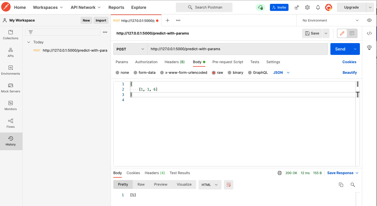
Figure 3.8 – Calling the endpoint predict-with-params from Postman

We see from Figure 3.8, that we got the response [1]. We will get the same result from both endpoints, as we copied the model from the first training to the model server and the params to the param store.

2. Now let’s try to retrain the model with different data. The training code now looks like the following:

   X = [[8, 4, 2], [5, 1, 3], [5, 1, 3]]

   Y = [2, 1, 0]

   model = tree.DecisionTreeClassifier()

   model.fit(X, Y)

Now we get the response [0] from the line print(model.predict([[1, 1, 6]])).

3. Now let’s invoke both endpoints from Postman.

First, let’s call the endpoint "/predict-with-full-model". This model loads the full model along with the parameters from the model server. As we have not copied the updated model to the model server, we still get the output [1] for the input [[1, 1, 6]], as shown in Figure 3.9.

Figure 3.9 – Calling the endpoint “/predict-with-full-model” does not reflect the second training

4. Now let’s call the other endpoint, which loads the params from the param store. The response is shown in Figure 3.10. Here, we get the response [0] from the served model. This is exactly the same as we got during testing after the second training was done.

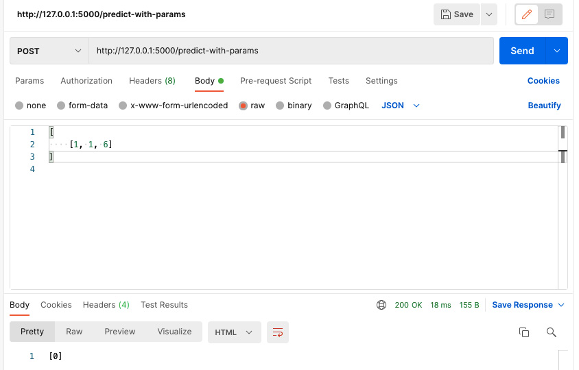
Figure 3.10 – Calling the endpoint “/predict-with-params” reflects the updates due to the second training

We notice that the parameter decoupling helps to add consistency to the response.

Parameter decoupling can be more useful in neural networks. In neural networks, weights and biases are used as states and impact predictions. We can move these states to a state store.

5. For example, let’s take the DNN model we saw earlier and save the model using the following code snippet:

   model.save('saved_model')

This will save the model in a folder named saved_model, as shown in Figure 3.11.

Figure 3.11 – Saved Keras DNN model in the local workspace

We notice in Figure 3.11 that the saved_model folder contains a file called saved_model.pb, which stores the structure of the model. The variables folder contains the weights and biases of the model.

6. When we want to load the model, we can use the following command:

   model: tf.keras.models.Sequential = tf.keras.models.load_model('saved_model')

It will load the model structure from the saved_mode.pb file and load the weights from the variables folder.

7. We can just save the weights separately, using the following command:

   model.save_weights('mnist_weights')

This will save the weights and create two files in the same directory:

• mnist_weights.data*
• Mnitst_weights.index

8. If we want to replace the weights with weights from these two files, we need to use the following command:

   model.load_weights("mnist_weights")

The whole code snippet for loading the model and weights is as follows:

import tensorflow as tf
import tensorflow_datasets as tfds
(ds_train, ds_test), ds_info = tfds.load(
     'mnist',
     split=['train', 'test'],
     shuffle_files=True,
     as_supervised=True,
     with_info=True,
)
def normalize_img(image, label):
  """Normalizes images: `uint8` -> `float32`."""
  return tf.cast(image, tf.float32) / 255., label
ds_train = ds_train.map(
     normalize_img, num_parallel_calls=tf.data.AUTOTUNE)
ds_train = ds_train.cache()
print(ds_info.splits['train'].num_examples)
ds_train = ds_train.shuffle(ds_info.splits['train'].num_examples)
ds_train = ds_train.batch(128)
ds_train = ds_train.prefetch(tf.data.AUTOTUNE)
ds_test = ds_test.map(normalize_img)
ds_test = ds_test.batch(128)
model: tf.keras.models.Sequential = tf.keras.models.load_model('saved_model')
model.summary()
preds = model.predict(ds_test)
print(preds[0]) # prediction without loading weights separately
model.load_weights("mnist_weights")
preds = model.predict(ds_test)
print(preds[0]) # prediction with loading weights separately

We see that there are two print(pred[0]) statements. Before the last print statement, we load the weights of the model from the latest training. The outputs of the two print statements do not match. The output from the first print statement is shown here:

[2.1817669e-02 2.6139291e-04 6.7319870e-01 1.5672690e-01 2.3953454e-04
1.8283235e-02 2.0535434e-02 9.9055481e-04 1.0748719e-01 4.5936121e-04]

The output from the second print statement is different than the previous one:

[1.2448521e-03 4.2022881e-03 7.5482649e-01 2.8224552e-02 2.5956056e-04
5.9235198e-03 1.8221477e-01 4.1858567e-04 2.2648767e-02 3.6615722e-05]

These outputs may be different when you run your program. The point here is during the second prediction, we load the model weights from a separate decoupled location. This location could be a content server or web server. Before making predictions, the model will load the weights from this location and all the servers will stay in sync as this state store will be common to all the servers.

Summary

In this chapter, we have learned about stateful and stateless functions in more detail. We have seen how stateful serving can be problematic, causing impediments to scalable and resilient serving. Stateful serving can also violate fundamental computer science principles by causing servers to be out of sync. The response from servers will not be consistent once they are out of sync, violating the consistency principle.

We have discussed different kinds of states in machine learning models and how they impact inference. We also discussed that these models, with all these states, can be a big barrier to resilient and scalable serving.

We have seen some techniques to decouple states from ML models and have tried some demos using some dummy models by serving using the Flask API server.

In the next chapter, we will learn about continued model evaluation. We will discuss what the continuous model evaluation pattern is and why it is necessary, along with examples.