
Chapter 9: Natural Language Processing
In the previous chapter, we discussed using deep learning to not only address structured data in the form of tables but also sequence-based data where the order of the elements matters. In this chapter, we will be discussing another form of sequence-based data – text, within a field known as Natural Language Processing (NLP). We can define NLP as a subset of artificial intelligence that overlaps with both the realms of machine learning and deep learning, specifically when it comes to interactions between the areas of linguistics and computer science.
There are many well-known and well-documented applications and success stories of using NLP for various tasks. Products ranging from spam detectors all the way to document analyzers involve NLP to some extent. Throughout this chapter, we will explore several different areas and applications involving NLP.
As we have observed with many other areas of data science we have explored thus far, the field of NLP is just as vast and sparse, with endless tools and applications that a single book would never be able to fully cover. Throughout this chapter, we will aim to highlight as many of the most common and useful applications you will likely encounter as we can.
Throughout this chapter, we will explore many of the popular areas relating to NLP from the perspective of both structured and unstructured data. We will explore several topics, such as entity recognition, sentence analysis, topic modeling, sentiment analysis, and natural language search engines.
In this chapter, we will cover the following topics:
- Introduction to NLP
- Getting started with NLP using NLTK and SciPy
- Working with structured data
- Tutorial – abstract clustering and topic modeling
- Working with unstructured data
- Tutorial – developing a scientific data search engine using transformers
With these objectives in mind, let's go ahead and get started.
Introduction to NLP
Within the scope of biotechnology, we often turn to NLP for numerous reasons, which generally involve the need to organize data and develop models to find answers to scientific questions. As opposed to the many other areas we have investigated so far, NLP is unique in the sense that we focus on one type of data at hand: text data. When we think of text data within the realm of NLP, we can divide things into two general categories: structured data and unstructured data. We can think of structured data as text fields living within tables and databases in which items are organized, labeled, and linked together for easier retrieval, such as a SQL or DynamoDB database. On the other hand, we have what is known as unstructured data such as documents, PDFs, and images, which can contain static content that is neither searchable nor easily accessible. An example of this can be seen in the following diagram:
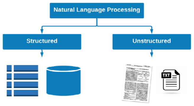
Figure 9.1 – Structured and unstructured data in NLP
Often, we wish to use documents or text-based data for various purposes, such as the following:
- Generating insights: Looking for trends, keywords, or key phrases
- Classification: Automatically labeling documents for various purposes
- Clustering: Grouping documents together based on features and characteristics
- Searching: Quickly finding important knowledge in historical documents
In each of these examples, we would need to take our data from unstructured data and move it toward a structured state to implement these tasks. In this chapter, we will look at some of the most important and useful concepts and tools you should know about concerning the NLP space.
Getting started with NLP using NLTK and SciPy
There are many different NLP libraries available in the Python language that allow users to accomplish a variety of different tasks for analyzing data, generating insights, or preparing predictive models. To begin our journey in the realm of NLP, we will take advantage of two popular libraries known as NLTK and SciPy. We will begin by importing these two libraries:
import nltk
import scipy
Often, we will want to parse and analyze raw pieces of text for particular purposes. Take, for example, the following paragraph regarding the field of biotechnology:
paragraph = """Biotechnology is a broad area of biology, involving the use of living systems and organisms to develop or make products. Depending on the tools and applications, it often overlaps with related scientific fields. In the late 20th and early 21st centuries, biotechnology has expanded to include new and diverse sciences, such as genomics, recombinant gene techniques, applied immunology, and development of pharmaceutical therapies and diagnostic tests. The term biotechnology was first used by Karl Ereky in 1919, meaning the production of products from raw materials with the aid of living organisms."""
Here, there is a single string that's been assigned to the paragraph variable. Paragraphs can be separated into sentences using the sent_tokenize() function, as follows:
from nltk.tokenize import sent_tokenize
nltk.download('popular')
sentences = sent_tokenize(paragraph)
print(sentences)
Upon printing these sentences, we will get the following output:

Figure 9.2 – A sample list of sentences that were split from the initial paragraph
Similarly, we can use the word_tokenize() function to separate the paragraph into individual words:
from nltk.tokenize import word_tokenize
words = word_tokenize(sentences[0])
print(words)
Upon printing the results, you will get a list similar to the one shown in the following screenshot:
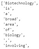
Figure 9.3 – A sample list of words that were split from the first sentence
Often, we will want to know the part of speech for a given word in a sentence. We can use the pos_tag() function on a given string to do this – in this case, the first sentence of the paragraph:
tokens = word_tokenize(sentences[0])
tags = nltk.pos_tag(tokens)
print(tags)
Upon printing the tags, we get a list of sets where the word or token is listed on the left and the associated part of speech is on the right. For example, Biotechnology and biology were tagged as proper nouns, whereas involving and develop were tagged as verbs. We can see an example of these results in the following screenshot:
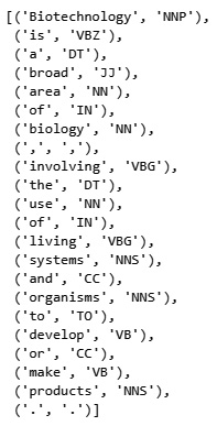
Figure 9.4 – Results of the part-of-speech tagging method
In addition to understanding the parts of speech, we often want to know the frequency of the given words in a particular string of text. For this, we could either tokenize the paragraph into words, group by word, count the instances and plot them, or use NLTK's built-in functionality:
freqdist = nltk.FreqDist(word_tokenize(paragraph))
import matplotlib.pyplot as plt
import seaborn as sns
plt.figure(figsize=(10,3))
plt.xlabel("Samples", fontsize=20)
plt.xticks(fontsize=14)
plt.ylabel("Counts", fontsize=20)
plt.yticks(fontsize=14)
sns.set_style("darkgrid")
freqdist.plot(30,cumulative=False)
By doing this, you will receive the following output:
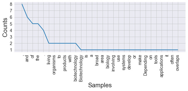
Figure 9.5 – Results of calculating the frequency (with stop words)
Here, we can see that the most common elements are commas, periods, and other irrelevant words. Words that are irrelevant to any given analysis are known as stop words and are generally removed as part of the preprocessing step. Punctuation, on the other hand, can be handled with regex. Let's go ahead and prepare a function to clean our text:
from nltk.corpus import stopwords
from nltk.tokenize import word_tokenize
nltk.download('punkt')
nltk.download('stopwords')
import re
STOP_WORDS = stopwords.words()
def cleaner(text):
text = text.lower() #Convert to lower case
text = re.sub("[^a-zA-Z]+", ' ', text) # Only keep text, remove punctuation and numbers
text_tokens = word_tokenize(text) #Tokenize the words
tokens_without_sw = [word for word in text_tokens if not word in STOP_WORDS] #Remove the stop words
filtered_sentence = (" ").join(tokens_without_sw) # Join all the words or tokens back to a single string
return filtered_sentence
There are four main steps within this function. First, we convert the text into lowercase for consistency; then, we use regex to remove all punctuation and numbers. After, we split the string into individual tokens and remove the words if they are in our list of stop words, before finally joining the words back together into a single string.
Important note
Please note that text cleaning scripts are often specific to the use case in the sense that not all use cases require the same steps.
Now, we can apply the cleaner function to our paragraph:
clean_paragraph = cleaner(paragraph)
clean_paragraph
We can see the output of this function in the following screenshot:
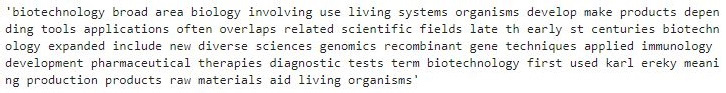
Figure 9.6 – Output of the text cleaning function
Upon recalculating the frequencies with the clean text, we can replot the data and view the results:
import matplotlib.pyplot as plt
import seaborn as sns
plt.figure(figsize=(10,3))
plt.xlabel("Samples", fontsize=20)
plt.xticks(fontsize=14)
plt.ylabel("Counts", fontsize=20)
plt.yticks(fontsize=14)
sns.set_style("darkgrid")
freqdist.plot(30,cumulative=False)
The output of this code can be seen in the following screenshot:
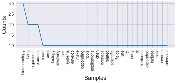
Figure 9.7 – Results of calculating the frequency (without stop words)
As we begin to dive deeper into our text, we will often want to tag items not only by their parts of speech, but also by their entities, allowing us to parse dates, names, and many others in a process known as Named Entity Recognition (NER). To accomplish this, we can make use of the spacy library:
import spacy
spacy_paragraph = nlp(paragraph)
spacy_paragraph = nlp(paragraph)
print([(X.text, X.label_) for X in spacy_paragraph.ents])
Upon printing the results, we obtain a list of items and their associated entity tags. Notice that the model not only picked up the year 1919 as a DATE entity but also picked up descriptions such as 21st centuries as DATE entities:
Figure 9.8 – Results of the NER model showing the text and its subsequent tag
We can also display the tags from a visual perspective within Jupyter Notebook using the render function:
from spacy import displacy
displacy.render(nlp(str(sentences)), jupyter=True, style='ent')
Upon executing this code, we will receive the original paragraph, which has been color-coded based on the identified entity tags, allowing us to view the results visually:
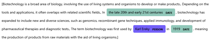
Figure 9.9 – Results of the NER model when rendered in Jupyter Notebook
We can also use SciPy to implement a visual understanding of our text when it comes to parts of speech using the same render() function:
displacy.render(nlp(str(sentences[0])), style='dep', jupyter = True, options = {'distance': 120})
We can see the output of this command in the following diagram:
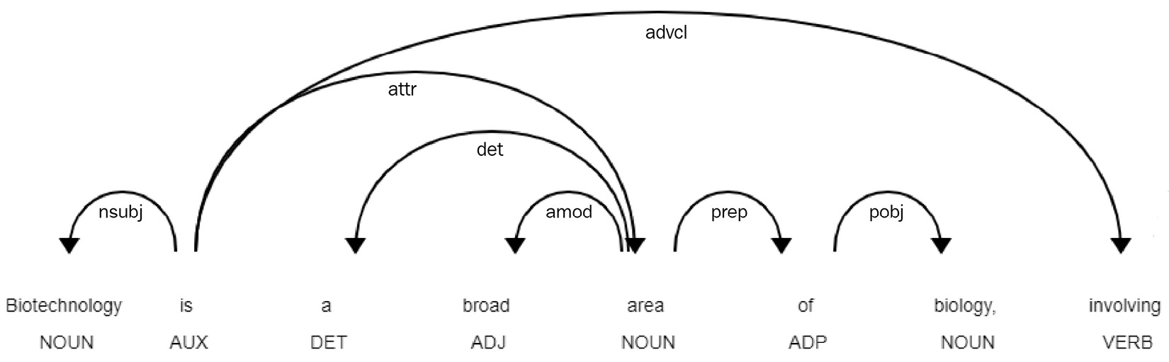
Figure 9.10 – Results of the POS model when rendered in Jupyter Notebook
This gives us a great way to understand and visualize the structure of a sentence before implementing any NLP models. With some of the basic analysis out of the way, let's go ahead and explore some applications of NLP using structured data.
Working with structured data
Now that we have explored some of the basics of NLP, let's dive into some more complex and common use cases that are often observed in the biotech and life sciences fields. When working with text-based data, it is much more common to work with larger datasets rather than single strings. More often than not, we generally want these datasets to involve scientific data regarding specific areas of interest relating to a particular research topic. Let's go ahead and learn how to retrieve scientific data using Python.
Searching for scientific articles
To programmatically retrieve scientific publication data using Python, we can make use of the pymed library from PubMed (https://pubmed.ncbi.nlm.nih.gov/). Let's go ahead and build a sample dataset:
- First, let's import our libraries and instantiate a new PubMed object:
from pymed import PubMed
pubmed = PubMed()
- Next, we will need to define and run our query. Let's go ahead and search for all the items related to monoclonal antibodies and retrieve 100 results:
query = "monoclonal antibody"
results = pubmed.query(query, max_results=100)
- With the results found, we can iterate over our results to retrieve all the available fields for each of the given articles:
articleList = []
for article in results:
articleDict = article.toDict()
articleList.append(articleDict)
- Finally, we can go ahead and convert our list into a DataFrame for ease of use:
df = pd.DataFrame(articleList)
df.head()
The following is the output:

Figure 9.11 – A DataFrame showing the results of the PubMed search
With the final step complete, we have a dataset full of scientific abstracts and their associated metadata. In the next section, we will explore this data in more depth and develop a few visuals to represent it.
Exploring our datasets
Now that we have some data to work with, let's go ahead and explore it. If you recall from many of the previous chapters, we often explore our numerical datasets in various ways. We can group columns, explore trends, and find correlations – tasks we cannot necessarily do when working with text. Let's implement a few NLP methods to explore data in a slightly different way.
Checking string lengths
Since we have our dataset structured within a pandas DataFrame, one of the first items we generally want to explore is the distribution of string lengths for our text-based data. In the current dataset, the two main columns containing text are title and abstract – let's go ahead and plot the distribution of lengths:
sns.displot(df.abstract.str.len(), bins=25)
sns.displot(df.title.str.len(), bins=25)
The following is the output:
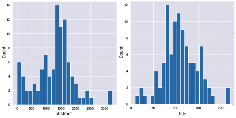
Figure 9.12 – Frequency distributions of the average length of abstracts (left) and titles (right)
Here, we can see that the average length of most abstracts is around 1,500 characters, whereas titles are around 100. Since the titles may contain important keywords or identifiers for a given article, similar to that of the abstracts, it would be wise to combine the two into a single column to analyze them together. We can simply combine them using the + operator:
df["text"] = df["title"] + " " + df["abstract"]
df[["title", "abstract", "text"]]
We can see this new column in the following screenshot:
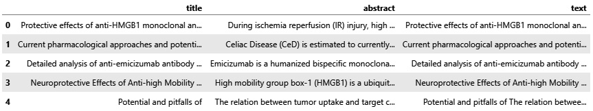
Figure 9.13 – A sample DataFrame showing the title, abstract, and text columns
Using the mean() function on each of the columns, we can see that the titles have, on average, 108 characters, the abstracts have 1,277 characters, and the combined text column has 1,388 characters.
Similar to other datasets, we can use the value_counts() function to get a quick sense of the most common words:
df.text.str.split(expand=True).stack().value_counts()
Immediately, we notice that our dataset is flooded with stop words:

Figure 9.14 – A sample of the most frequent words in the dataset
We can implement the same cleaner function as we did previously to remove these stop words and any other undesirable values. Note that some of the cells within the DataFrame may be empty, depending on the query made and the results returned. We'll take a closer look at this in the next section.
Cleaning text data
We can add a quick check at the top of the function by checking the type of the value to ensure that no errors are encountered:
from nltk.corpus import stopwords
STOP_WORDS = stopwords.words()
def cleaner(text):
if type(text) == str:
text = text.lower()
text = re.sub("[^a-zA-Z]+", ' ', text)
text_tokens = word_tokenize(text)
tokens_without_sw = [word for word in text_tokens if not word in STOP_WORDS]
filtered_sentence = (" ").join(tokens_without_sw)
return filtered_sentence
We can quickly test this out on a sample string to test the functionality:
cleaner("Biotech in 2021 is a wonderful field to work and study in!")
The output of this function can be seen in the following screenshot:
Figure 9.15 – Results of the cleaning function
With the function working, we can go ahead and apply this to the text column within the DataFrame and create a new column consisting of the cleaned text using the apply() function, which allows us to apply a given function iteratively down through all rows of a DataFrame:
df["clean_text"] = df["text"].apply(lambda x: cleaner(x))
We can check the performance of our function by checking the columns of interest:
df[["text", "clean_text"]].head()
We can see these two columns in the following screenshot:

Figure 9.16 – A DataFrame showing the original and cleaned texts
If we go ahead and check value_counts()of the clean_text column, as we did previously, you will notice that the stop words were removed and that more useful keywords are now populated at the top.
Creating word clouds
Another popular and useful method to get a quick sense of the content for a given text-based dataset is by using word clouds. Word clouds are images that are populated with the content of a dataset in which words are rendered in larger fonts when they are more frequent, and smaller fonts when they are less frequent. To accomplish this, we can make use of the wordclouds library:
- First, we need to import the function and then create a wordcloud object that we will specify a number of parameters in. We can adjust the dimensions of the image, colors, and the data as follows:
from wordcloud import WordCloud, STOPWORDS
plt.figure(figsize=(20,10))
# Drop nans
df2 = df[["clean_text"]].dropna()
# Create word cloud
wordcloud = WordCloud(width = 5000,
height = 3000,
random_state=1,
background_color='white',
colormap='Blues',
collocations=False,
stopwords = STOPWORDS).generate(' '.join(df2['clean_text']))
- Now, we can use the imshow() function from matplotlib to render the image:
plt.figure( figsize=(15,10) )
plt.imshow(wordcloud)
The following is the output:
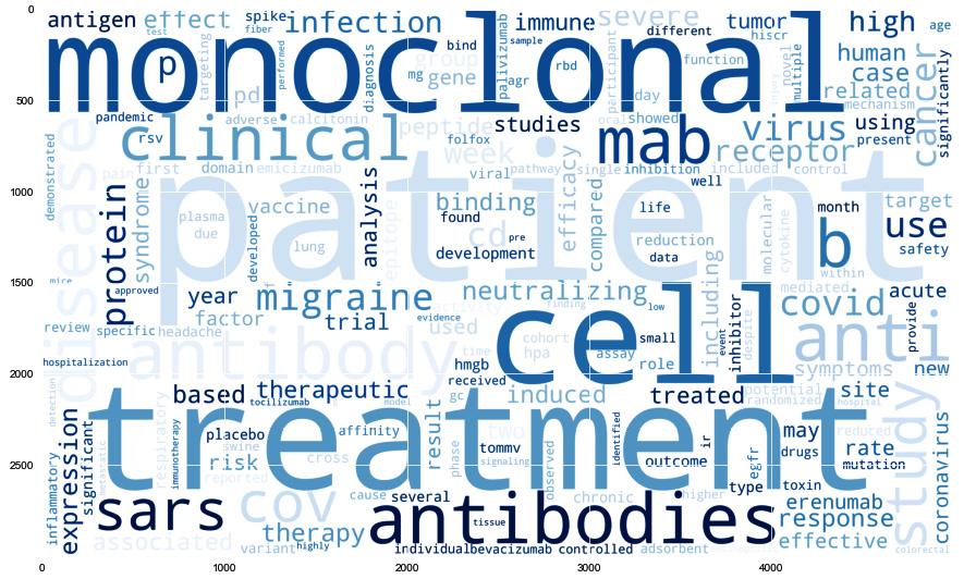
Figure 9.17 – A word cloud representing the frequency of words in the dataset
In this section, we investigated a few of the most popular methods for quickly analyzing text-based data as a preliminary step before performing any type of rigorous analysis or model development process. In the next section, we will train a model using this dataset to investigate topics.
Tutorial – clustering and topic modeling
Similar to some of the previous examples we have seen so far, much of our data can either be classified in a supervised setting or clustered in an unsupervised one. In most cases, text-based data is generally made available to us in the form of real-world data in the sense that it is in a raw and unlabeled form.
Let's look at an example where we can make sense of our data and label it from an unsupervised perspective. Our main objective here will be to preprocess our raw text, cluster the data into five clusters, and then determine the main topics for each of those clusters. If you are following along using the provided code and documentation, please note that your results may vary as the dataset is dynamic, and its contents change as new data is populated into the PubMed database. I would urge you to customize the queries to topics that interest you. With that in mind, let's go ahead and begin.
We will begin by querying some data using the pymed library and retrieving a few hundred abstracts and titles to work with:
def dataset_generator(query, num_results, ):
results = pubmed.query(query, max_results=num_results)
articleList = []
for article in results:
articleDict = article.toDict()
articleList.append(articleDict)
print(f"Found {len(articleList)} results for the query '{query}'.")
return pd.DataFrame(articleList)
Instead of making a single query, let's make a few and combine the results into a single DataFrame:
df1 = dataset_generator("monoclonal antibodies", 600)
df2 = dataset_generator("machine learning", 600)
df3 = dataset_generator("covid-19", 600)
df4 = dataset_generator("particle physics", 600)
df = pd.concat([df1, df2, df3, df4])
Taking a look at the data, we can see that some of the cells have missing (nan) values. Given that our objective concerns the text-based fields only (titles and abstracts), let's limit the scope of any cleaning methods to those columns alone:
df = df[["title", "abstract"]]
Given that we are concerned with the contents of each article as a whole, we can combine the titles and abstracts together into a new column called text:
df["text"] = df["title"] + " " + df["abstract"]
df = df.dropna()
print(df.shape)
Taking a look at the dataset, we can see that we have 560 rows and 3 columns. Scientific articles can be very descriptive, encompassing many stop words. Given that our objective here is to detect topics that are represented by keywords, let's remove any punctuation, numerical values, and stopwords from our text:
def cleaner(text):
if type(text) == str:
text = text.lower()
text = re.sub("[^a-zA-Z]+", ' ', text)
text_tokens = word_tokenize(text)
tokens_without_sw = [word for word in text_tokens if not word in STOP_WORDS]
filtered_sentence = (" ").join(tokens_without_sw)
return filtered_sentence
df["text"] = df["text"].apply(lambda x: cleaner(x))
We can check the average number of words per article before and after implementing the script to ensure that the data was cleaned. In our case, we can see that we started with an average of 190 words and ended up with an average of 123.
With the data now clean, we can go ahead and extract our features. We will use a relatively simple and common method known as TFIDF – a measure of originality of words in which each word is compared to the number of times it appears in an article, relative to the number of articles the same word appears in. We can think of TFIDF as two separate items – Term Frequency (TF) and Inverse Document Frequency (IDF) – which we can represent as follows:

In the preceding equation, t is the term or keyword, while d is the document or – in our case – the article. The main idea here is to capture important keywords that would be descriptive as main topics but ignore those that appear in almost every article. We will begin by importing TfidfVectorizer from sklearn:
from sklearn.feature_extraction.text import TfidfVectorizer
Next, we will convert our text-based data into numerical features by fitting our dataset and transforming the values:
vectors = TfidfVectorizer(stop_words="english", max_features=5500)
vectors.fit(df.text.values)
features = vectors.transform(df.text.values)
We can check the shape of the features variable to confirm that we have 560 rows, just as we did before applying TFIDF, and 5,500 columns worth of features to go with it. Next, we can go ahead and cluster our documents using one of the many clustering methods we have explored so far.
Let's implement MiniBatchKMeans and specify 4 as the number of clusters we want to retrieve:
from sklearn.cluster import MiniBatchKMeans
cls = MiniBatchKMeans(n_clusters=4)
cls.fit(features)
When working with larger datasets, especially in production, it is generally advisable to avoid using pandas DataFrames as there are more efficient methods available, depending on the processes you need to implement. Given that we are only working with 560 rows of data, and our objective is to cluster our data and retrieve topics, we will once again make use of DataFrames to manage our data. Let's go ahead and add our predicted clusters to our DataFrame:
df["cluster"] = cls.predict(features)
df[["text", "cluster"]].head()
We can see the output of this command in the following screenshot:

Figure 9.18 – A DataFrame showing the cleaned texts and their associated clusters
With the data clustered, let's plot this data in a 2D scatterplot. Given that we have several thousand features, we can make use of the PCA algorithm to reduce these down to only two features for our visualization:
from sklearn.decomposition import PCA
pca = PCA(n_components=2)
pca_features_2d = pca.fit_transform(features.toarray())
pca_features_2d_centers = pca.transform(cls.cluster_centers_)
Let's go ahead and add these two principal components to our DataFrame:
df["pc1"], df["pc2"] = pca_features_2d[:,0], pca_features_2d[:,1]
df[["text", "cluster", "pc1", "pc2"]].head()
We can see the output of this command in the following screenshot:
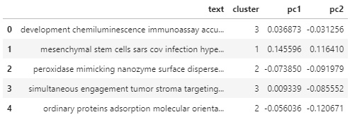
Figure 9.19 – A DataFrame showing the texts, clusters, and principal components
Here, we can see that each row of text now has a cluster, as well as a set of coordinates, in the form of principal components. Next, we will plot our data and color by cluster:
plt.figure(figsize=(15,8))
new_cmap = matplotlib.colors.LinearSegmentedColormap.from_list("mycmap", colors)
plt.scatter(df["pc1"], df["pc2"], c=df["cluster"], cmap=new_cmap)
plt.scatter(pca_features_2d_centers[:, 0], pca_features_2d_centers[:,1], marker='*', s=500, c='r')
plt.xlabel("PC1", fontsize=20)
plt.ylabel("PC2", fontsize=20)
Upon executing this code, we will get the following output:
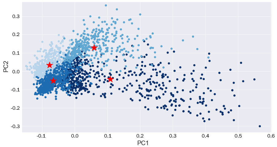
Figure 9.20 – A scatterplot of the principal components colored by cluster, with stars representing the cluster centers
Here, we can see that there seems to be some adequate separation between clusters! The two clusters on the far left seem to have smaller variance in their distributions, whereas the other two are much more spread out. Given that we reduced a considerable number of features down to only two principal components, it makes sense that there is a certain degree of overlap between them, especially given the fact that all the articles were scientific.
Now, let's go ahead and calculate some of the most prominent topics that were found in our dataset:
- First, we will begin by implementing TFIDF:
from sklearn.feature_extraction.text import CountVectorizer, TfidfVectorizer
vectors = TfidfVectorizer(max_features=5500, stop_words="english")
nmf_features = vectors.fit_transform(df.text)
- Next, we will reduce the dimensionality. However, this time, we will use Non-Negative Matrix Factorization (NMF) to reduce our data instead of PCA. We will need to specify the number of topics we are interested in:
from sklearn.decomposition import NMF
n_topics = 10
cls = NMF(n_components=n_topics)
cls.fit(features)
- Now, we can specify the number of keywords to retrieve per topic. After that, we will iterate over the components and retrieve the keywords of interest:
num_topic_words = 3
feature_names = vectors.get_feature_names()
for i, j in enumerate(cls.components_):
print(i, end=' ')
for k in j.argsort()[-1:-num_topic_words-1:-1]:
print(feature_names[k], end=' ')
Upon executing this loop, we retrieve the following as output:

Figure 9.21 – Top 10 topics of the dataset, each represented by three keywords
We can use these topic modeling methods to extract insights and trends from the dataset, allowing users to have high-level interpretations without the need to dive into the datasets as a whole. Throughout this tutorial, we examined one of the classical methods for clustering and topic modeling: using TFIDF and NMF. However, many other methods exist that use language models, such as BERT and BioBERT and libraries such as Gensim and LDA. If this is an area you find interesting, I highly urge you to explore these libraries for more information.
Often, you will not have your data already existing in a usable format. In this tutorial, we had our dataset structured within a DataFrame, ready for use to slice and dice. However, in many cases, our data of interest will be unstructured, such as in PDFs. We will explore how to handle situations such as these in the next section.
Working with unstructured data
In the previous section, we explored some of the most common tasks and processes that are conducted when handing text-based data. More often than not, you will find that the data you work with is generally not of a structured nature, or perhaps not of a digital nature. Take, for example, a company that has decided to move all printed documents to a digital state. Or perhaps a company that maintains a large repository of documents, none of which are structured or organized. For tasks such as these, we can rely on several AWS products to come to our rescue. We will explore two of the most useful NLP tools in the next few sections.
OCR using AWS Textract
In my opinion, one of the most useful tools available within AWS is an Optical Character Recognition (OCR) tool known as AWS Textract. The main idea behind this tool is to enable users to extract text, tables, and other useful items from images or static PDF documents using pre-built machine learning models implemented within Textract.
For example, users can upload images or scanned PDF documents to Textract that are otherwise unsearchable and extract all the text-based content from them, as shown in the following diagram:

Figure 9.22 – A schematic showing structuring raw PDFs into organized digital text
In addition to extracting text, users can extract key-value pairs such as those found in both printed and handwritten forms:
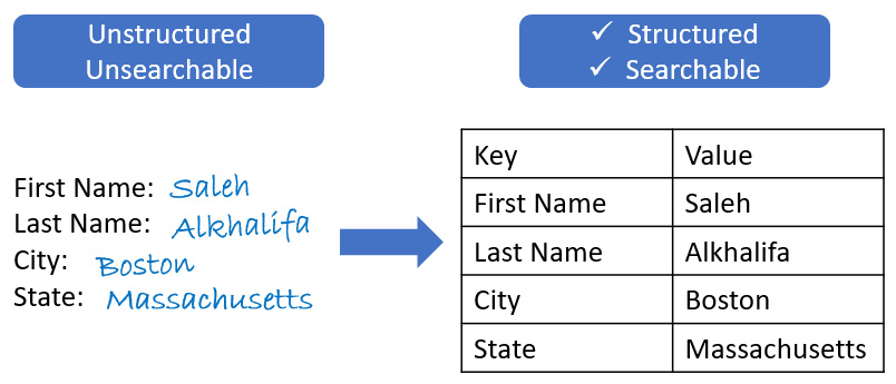
Figure 9.23 – A schematic showing the structuring of handwritten data to organized tables
To use Textract in Python, we will need to use an AWS Python library known as boto3. We can install Boto3 using pip. When using Boto3 within SageMaker, you will not be required to use any access keys to utilize the service. However, if you are using a local implementation of Jupyter Notebook, you will need to be able to authenticate using access keys. Access keys can easily be created in a few simple steps:
- Navigate to the AWS console and select IAM from the Services menu.
- Under the Access Management tab on the left, click on Users, then Add Users.
- Go ahead and give your user a name, such as ml-biotech-user, and enable the Programmatic access option:
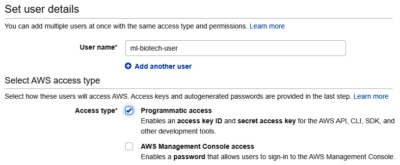
Figure 9.24 – Setting the username for AWS IAM roles
- Next, select the Attach existing policies directly option at the top and add the policies of interest. Go ahead and add Textract, Comprehend, and S3 as we will require all three for the role:
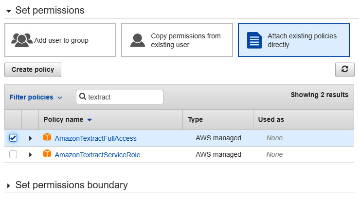
Figure 9.25 – Setting the policies for AWS IAM roles
- After labeling your new user with some descriptive tags, you will gain access to two items: your access key ID and AWS secret access k. Be sure to copy those two items to a safe space. For security, you will not be able to retrieve them from AWS after leaving this page.
Now that we have our access keys, let's go ahead and start implementing Textract on a document of interest. We can complete this in a few steps.
- First, we will need to upload our data to our S3 bucket. We can recycle the same S3 bucket we used earlier in this book. We will need to specify our keys, and then connect to AWS using the Boto3 client:
AWS_ACCESS_KEY_ID = "add-access-key-here"
AWS_SECRET_ACCESS_KEY = "add-secret-access-key-here"
AWS_REGION = "us-east-2"
s3_client = boto3.client('s3', aws_access_key_id=AWS_ACCESS_KEY_ID, aws_secret_access_key=AWS_SECRET_ACCESS_KEY, region_name=AWS_REGION)
- With our connection set up, we can go ahead and upload a sample PDF file. Note that you can submit PDFs as well as image files (PNG). Let's go ahead and upload our PDF file using the upload_fileobj() function:
with open("Monoclonal Production Article.pdf", "rb") as f:
s3_client.upload_fileobj(f, "biotech-machine-learning", "pdfs/Monoclonal Production Article.pdf")
- With our PDF now uploaded, we can use Textract. First, we will need to connect using the Boto3 client. Note that we changed the desired resource from 's3' to 'textract' since we are using a different service now:
textract_client = boto3.client('textract', aws_access_key_id=AWS_ACCESS_KEY_ID, aws_secret_access_key=AWS_SECRET_ACCESS_KEY, region_name=AWS_REGION)
- Next, we can send our file to Textract using the start_document_text_detection() method, where we specify the name of the bucket and the name of the document:
response = textract_client.start_document_text_detection(
DocumentLocation={'S3Object': {'Bucket': "biotech-machine-learning", 'Name': "pdfs/Monoclonal Production Article.pdf"} })
- We can confirm that the task was started successfully by checking the status code in the response variable. After a few moments (depending on the duration of the job), we retrieve the results by specifying JobId:
results = textract_client.get_document_text_detection(JobId=response["JobId"])
Immediately, we will notice that the results variable is simply one large JSON that we can parse and iterate over. Notice that the structure of the JSON is quite complex and detailed.
- Finally, we can gather all the text by iterating over Blocks and collecting all the texts for blocks of the LINE type:
documentText = ""
for item in results["Blocks"]:
if item["BlockType"] == "LINE":
documentText = documentText + item["Text"]
If you print the documentText variable, you will see all of the text that was successfully collected from that document! Textract can be an extremely useful tool for moving documents from an unstructured and unsearchable state to a more structured and searchable state. Often, most text-based data will exist in an unstructured format, and you will find Textract to be one of the most useful resources for these types of applications. Textract is generally coupled with other AWS resources to maximize the utility of the tool, such as DynamoDB for storage or Comprehend for analysis. We will explore Comprehend in the next section.
Entity recognition using AWS Comprehend
Earlier in this chapter, we implemented a NER model using the SciPy library to detect entities in a given section of text. Now, let's explore a more powerful implementation of NER known as AWS Comprehend. Comprehend is an NLP service that's designed to discover insights in unstructured text data, allowing users to extract key phrases, calculate sentiment, identify entities, and much more. Let's go ahead and explore this tool.
Similar to other AWS resources, we will need to connect using the boto3 client:
comprehend_client = boto3.client('comprehend', aws_access_key_id=AWS_ACCESS_KEY_ID, aws_secret_access_key=AWS_SECRET_ACCESS_KEY, region_name=AWS_REGION)
Next, we can go ahead and use the detect_entities() function to identify entities in our text. We can use the documentText string we generated using Textract earlier:
response = comprehend_client.detect_entities(
Text=documentText[:5000],
LanguageCode='en',
)
print(response["Entities"])
Upon printing the response, we will see the results for each of the entities that were detected in our block of text. In addition, we can organize the results in a DataFrame:
pd.DataFrame(response["Entities"]).sort_values(by='Score', ascending=False).head()
Upon sorting the values by score, we can see our results listed in a structured manner:
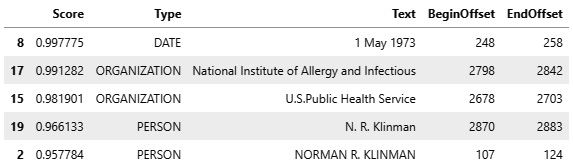
Figure 9.26 – A sample DataFrame showing the results of the AWS Comprehend entities API
In addition to entities, Comprehend can also detect key phrases within text:
response = comprehend_client.detect_key_phrases(
Text=documentText[:5000],
LanguageCode='en',
)
response["KeyPhrases"][0]
Upon printing the first item in the list, we can see the score, phrase, and position in the string:
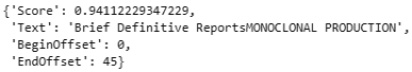
Figure 9.27 – Results of the AWS Comprehend key phrases API
In addition, we can also detect the sentiment using the detect_sentiment() function:
response = comprehend_client.detect_sentiment(
Text=documentText[:5000],
LanguageCode='en',
)
print(response)
We can print the response variable to get the results of the string. We can see that the sentiment was noted as neutral, which makes sense for a statement concerning scientific data that is generally not written with a positive or negative tone:

Figure 9.28 – Results of the AWS Comprehend sentiment API
Lastly, Comprehend can also detect dominant languages within text using the detect_dominant_language() function:
response = comprehend_client.detect_dominant_language(
Text=documentText[:5000],
)
response
Here, we can see that, upon printing the response, we get a sense of the language, as well as the associated score or probability from the model:
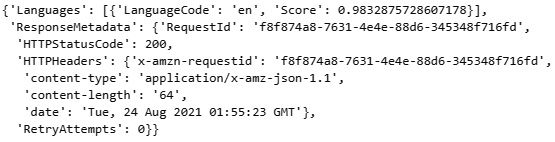
Figure 9.29 – Results of the AWS Comprehend language detection API
AWS Textract and AWS Comprehend are two of the top NLP tools available today and have been instrumental in structuring and analyzing vast amounts of unstructured text documents. Most NLP-based applications today generally use at least one, if not both, of these types of technologies. For more information about Textract and Comprehend, I highly recommend that you visit the AWS website (https://aws.amazon.com/).
So far, we have learned how to analyze and transform text-based data, especially when it comes to moving data from an unstructured state to a more structured state. Now that the documents are more organized, the next step is to be able to use them in one way or another, such as through a search engine. We will learn how to create a semantic search engine using transformers in the next section.
Tutorial – developing a scientific data search engine using transformers
So far, we have looked at text from a word-by-word perspective in the sense that we kept our text as is, without the need to convert or embed it in any way. In some cases, converting words into numerical values or embeddings can open many new doors and unlock many new possibilities, especially when it comes to deep learning. Our main objective within this tutorial will be to develop a search engine to find and retrieve scientific data. We will do so by implementing an important and useful deep learning NLP architecture known as a transformer. The main benefit here is that we will be designing a powerful semantic search engine in the sense that we can now search for ideas or semantic meaning rather than only keywords.
We can think of transformers as deep learning models designed to solve sequence-based tasks using a mechanism known as self-attention. We can think of self-attention as a method to help relate different portions of text within a sentence or embedding in an attempt to create a representation. Simply put, the model attempts to view sentences as ideas, rather than a collection of single words.
Before we begin to work with transformers, let's talk a little more about the idea of embeddings. We can think of embeddings as low-dimensional numerical values or vectors of continuous numbers representing an item, which in our case would be a word or sentence. We commonly convert words and sentences into embeddings to allow models to carry out machine learning tasks more easily when working with larger datasets. Within the context of NLP and neural networks, there are three main reasons embeddings are used:
- To reduce the dimensionality of large segments of text data
- To compute the similarity between two different texts
- To visualize relationships between portions of text
Now that we have gained a better sense of embeddings and the role they play in NLP, let's go ahead and get started with a real-world example of a scientific search engine. We will begin by importing a few libraries that we will need:
import scipy
import torch
import pandas as pd
from sentence_transformers import SentenceTransformer, util
To create our embeddings, we will need a model. We have the option to create a customized model concerning our dataset. The benefit here is that our results would likely improve, given that the model was trained on text about our domain. Alternatively, we could use other pre-trained models available from the SentenceTransformer website (https://www.sbert.net/). Let's download one of these pre-trained models:
model = SentenceTransformer('msmarco-distilbert-base-v4')
Next, we can create a testing database and populate it with a few sentences:
database = df["abstract"].values
Next, we can call the encode() function to convert our list of strings into a list of embeddings:
database_embeddings = model.encode(database)
If we check the length of the database and the length of database_embeddings using the len() function, we will find that they both contain the same number of elements since there should be one embedding for every piece of text. If we print the contents of the first element of the embeddings database, we will find that the content is now simply a list of vectors:

Figure 9.30 – A view of an embedded piece of text
With each of our documents now embedded, the idea would be that a user would want to search for or query a particular phrase. We can take a user's query and encode it as we did with the others, but assign that value to a new variable that we will call query_embedding:
query = "One of the best discoveries were monoclonal antibodies"
query_embedding = model.encode(query)
With the query and sentences embedded, we can compute the distance between the items. The idea here is that documents that were more similar to the user's query would have shorter distances, and those that were less similar would have longer ones. Notice that we are using cosine here as a measure of distance, and therefore, similarity. We can use other methods as well, such as the euclidean distance:
import scipy
cos_scores = util.pytorch_cos_sim(query_embedding,
database_embeddings)[0]
Let's go ahead and prepare a single runSearch function that incorporates the query, the encoder, as well as a method to display our results. The process begins with a few print statements, and then encodes the new query into a variable called query_embedding. The distances are then calculated, and the results are sorted according to their distance. Finally, the results are iterated over and the scores, titles, and abstracts for each are printed:
def askQuestion(query, top_k):
print(f"#########################################")
print(f"#### {query} ####")
print(f"#########################################")
query_embedding = model.encode(query, convert_to_tensor=True)
cos_scores = util.pytorch_cos_sim(query_embedding,
database_embeddings)[0]
top_results = torch.topk(cos_scores, k=top_k)
for score, idx in zip(top_results[0], top_results[1]):
print("#### Score: {:.4f}".format(score))
print("#### Title: ", df.loc[float(idx)].title)
print("#### Abstract: ", df.loc[float(idx)].abstract)
print("#################################")
Now that we have prepared our function, we can call it with our query of interest:
query = ' What is known about the removal of harmful cyanobacteria?
askQuestion(query, 5)
Upon calling the function, we retrieve several results printed similarly. We can see one of the results in the following screenshot, showing us the score, title, and abstract properties of the article:
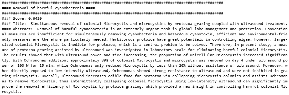
Figure 9.31 – Results of the semantic searching model for scientific text
With that, we have managed to successfully develop a semantic searching model capable of searching through scientific literature. Notice that the query itself is not a direct string match to the top result the model returned. Again, the idea here is not to match keywords but to calculate the distance between embeddings, which is representative of similarities.
Summary
In this chapter, we made an adventurous attempt to cover a wide range of NLP topics. We explored a range of introductory topics such as NER, tokenization, and parts of speech using the NLTK and spaCy libraries. We then explored NLP through the lens of structured datasets, in which we utilized the pymed library as a source for scientific literature and proceeded to analyze and clean the data in our preprocessing steps. Next, we developed a word cloud to visualize the frequency of words in a given dataset. Finally, we developed a clustering model to group our abstracts and a topic modeling model to identify prominent topics.
We then explored NLP through the lens of unstructured data in which we explored two common AWS NLP products. We used Textract to convert PDFs and images into searchable and structured text and Comprehend to analyze and provide insights. Finally, we learned how to develop a semantic search engine using deep learning transformers to find pertinent information.
What was particularly unique about this chapter is that we learned that text is a sequence-based type of data, which makes its uses and applications drastically different from many of the other datasets we had previously worked with. As companies across the world begin to migrate legacy documents into the digital space, the ability to search for documents and identify insights will be of great value. In the next chapter, we will examine another type of sequence-based data known as time series.