Chapter 3: Getting Started with SQL and Relational Databases

According to a recent article published in the Journal of Big Data Analytics and Its Applications, every 60 seconds on the internet, the following happens:

• 700,000 status updates are made.
• 11 million messages are sent.
• 170 million emails are received.
• 1,820 terabytes (TB) of new data is created.

It would be an understatement to claim that data within the business landscape is growing rapidly at an unprecedented rate. With this major explosion of information, companies around the globe are investing a great deal of capital in an effort to effectively capture, analyze, and deliver benefits from this data for the company. One of the main methods by which data can be managed and subsequently retrieved to provide actionable insights is through Structured Query Language (SQL).

Similar to how we used the Terminal command line to create directories, or Python to run calculations, you can use SQL to create and manage databases either locally on your computer or remotely in the cloud. SQL comes in many forms and flavors depending on the platform you choose to use, each of which contains a slightly different syntax. However, SQL generally consists of four main types of language statements, and these are outlined here:

• Data Manipulation Language (DML): Querying and editing data
• Data Definition Language (DDL): Querying and editing database tables
• Data Control Language (DCL): Creating roles and adding permissions
• Transaction Control Language (TCL): Managing database transactions

Most companies around the globe have their own separate best practices when it comes to DDL, DCL, and TCL and how databases are integrated into their enterprise systems. However, DML is generally the same and is often the main focus of any given data scientist. For these purposes, we will focus this chapter on applications relating to DML. By the end of this chapter, you will have gained a strong introduction to some of the most important database concepts, fully installed MySQL Workbench on your local machine, and deployed a full Amazon Web Services Relational Database Service (AWS RDS) server to host and serve your data. Note that all of these capabilities can later be recycled for your own endeavors. Let's get started!

We will cover the following topics in this chapter:

• Exploring relational databases
• Tutorial: Getting started with MySQL

Technical requirements

In this chapter, we will explore some of the main concepts behind relational databases, their benefits, and their applications. We will focus on one specific flavor of a relational database known as MySQL. We will use MySQL through its common User Interface (UI), known as MySQL Workbench. Whether you are using a Mac or a PC, the installation process for MySQL Workbench will be very similar, and we will walk through this together later in this chapter. This interface will allow you to interact with a database that can either be hosted on your local machine or far away in the cloud. Within this chapter, we will deploy and host our database server in the AWS cloud, and you will therefore need to have an AWS account. You can create an account by visiting the AWS website (https://aws.amazon.com/) and signing up as a new user.

Exploring relational databases

There are numerous types of databases—such as Object-Oriented (OO) databases, graph databases, and relational databases—each of which offers a particular capability.

OO databases are best used in conjunction with OO data. Data within these databases tends to consist of objects that contain members such as fields, functions, and properties; however, relations between objects are not well captured.

On the other hand, graph databases, as the name suggests, are best used with data consisting of nodes and edges. One of the most common applications for graph databases in the biotechnology sector is in small-molecule drug design. Molecules consist of nodes and edges that connect together in one form or another—these relations are best captured in graph databases. However, the relationships between molecules are not well captured here either.

Finally, relational databases, as the name suggests, are best used for databases in which relations are of major importance. One of the most important applications of relational databases in the biotechnology and healthcare sectors surrounds patient data. Relational databases are used with patient data due to its complex nature. Patients will have many different fields, such as name, address, location, age, and gender. A patient will be prescribed a number of medications, each medication containing its own sub-fields, such as a lot of numbers, quantities, and expiration dates. Each lot will have a manufacturing location, manufacturing date, and its associated ingredients, and each ingredient will have its own respective parameters, and so on. The complex nature of this data and its associated relations is best captured in a relational database.

Relational databases are standard digital databases that host tables in the form of columns and rows containing relations to one another. The relationship between two tables exists in the form of a Unique Identifier (UID) or Primary Key (PK). This key acts as a unique value for each of the rows within a single table, allowing users to match rows of one table to their respective rows in another table. The tables are not technically connected in any way; they are simply referenced or related to one another. Let's take a look at a simple example when it comes to patient data.

If we were to create a table of patient data containing patients' names, contact information, their pharmacies, and prescribing physicians, we would likely come up with a table similar to this:

Figure 3.1 – Table showing an example patient dataset

From an initial perspective, this table makes perfect sense. We have the patient's information listed nicely on the left, showing their name, address, and phone number. We also have the patient's respective Primary Care Physician (PCP), showing their associated names, addresses, and phone numbers. Finally, we also have the patient's respective pharmacy and their associated contact information. If we were trying to generate a dataset on all of our patients and their respective PCPs and pharmacies, this would be the perfect table to use. However, storing this data in a database would be a different story.

Notice that some of the PCP names and their contact information are repeated. Similarly, one of the pharmacies appears more than once in the sense that we have listed the name, address, and phone number twice in the same table. From the perspective of a three-row table, the repetition is negligible. However, as we scale this table from 3 patients to 30,000 patients, the repetition can be very costly from both a database perspective (to host the data) and a computational perspective (to retrieve the data).

Instead of having one single table host all our data, we can have multiple tables that when joined together temporarily for a particular purpose (such as generating a dataset) would be significantly less costly in the long run. This idea of splitting or normalizing data into smaller tables is the essence of relational databases. The main purpose of a relational database is to provide a convenient and efficient process to store and retrieve information while minimizing duplication as much as possible. To make this database more "relational", we can split the data into three tables—pharmacies, patients, and PCPs—so that we only store each entry once but use a system of keys to reference them.

Here, you can see a Unified Modeling Language (UML) diagram commonly used to describe relational databases. The connection between the tables indicated by the single line splitting into three others is a way to show a one-to-many relationship. In the following case, one pharmacy can have many patients and one PCP can have many patients, but a patient can have only one PCP and only one pharmacy. The ability to quickly understand a database design and translate that to a UML diagram (or vice versa) is an excellent skill to have when working with databases and is often regarded as an excellent interview topic—I actually received a question on this a few years ago:

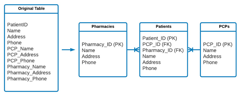
Figure 3.2 – The process of normalizing a larger table into smaller relational tables

The previous diagram provides a representation of how the original table can be split up. Notice that each of the tables has an ID; this ID is its UID or PK. Tables that are connected to others are referenced using a Foreign Key (FK). For example, a PCP can have multiple patients, but each patient will only have one PCP; therefore, each patient entry will need to have the FK of its associated PCP. Pretty interesting, huh?

The process of separating data in this fashion is known as database normalization, and there are a number of rules most relational databases must adhere to in order to be normalized properly. Data scientists do not often design major enterprise databases (we leave these tasks to database administrators). However, we often design smaller proof-of-concept databases that adhere to very similar standards. More often, we interact with significantly larger enterprise databases that are generally in a relational state or in the form of a data lake. In either case, a strong foundational knowledge of the structure and general idea behind relational databases is invaluable to any data scientist.

Database normalization

There are a number of rules we must consider when preparing a database that is normalized, often referred to as normal forms. There are three normal forms that we will briefly discuss within the context of relational databases, as follows:

First normal form

In order to satisfy the First Normal Form (1NF) of database normalization, the values in each of the cells must be atomic in the sense that each cell contains only one type of data. For example, a column containing addresses such as 5 First Street, Boston MA 02215 contains non-atomic data and violates this rule as it contains street numbers, street names, cities, states, and zip codes in one cell. We can normalize this data by splitting it into five columns, as follows:

Figure 3.3 – Table showing how addresses can be split into individual atomic cells

Now that we have gained a better understanding of the first form of data normalization, let's go ahead and explore the second form.

Second normal form

In order to satisfy the conditions of the Second Normal Form (2NF), the table must have a PK acting as a UID, and that all the fields excluding the PK must be functionally dependent on the entire key. For example, we can have a table with a list of all patients in the sense that the first name, last name, and phone number of the patients are dependent on the PK. This key represents the patient and nothing else. We can also have another table representing the PCPs, their locations, associated hospitals, and so on. However, it would not be appropriate from the perspective of database normalization to add this information to a table representing a patient.

To satisfy this condition with the patient database, we would need to split the table such that the patient data is in one table and the associated PCP is in a second table, connected via an FK, as we saw in the earlier example.

Third normal form

In order to satisfy the conditions for the Third Normal Form (3NF), we must satisfy the conditions of the 1NF and 2NF, in addition to ensuring that all the fields within the table are functionally independent of each other—in other words, no fields can be calculated fields. For example, a field titled Age with values of 27 years, 32 years, and 65 years of age would not be appropriate here as these are calculated quantities. Instead, a field titled Date of Birth with the associated dates could be used to satisfy this condition.

Most data scientists spend little time structuring major databases and normalizing them; however, a great deal of time is spent understanding database structures and forming queries to retrieve data correctly and efficiently. Therefore, a strong foundational understanding of databases will always be useful.

Although database administrators and data engineers tend to spend more time on structuring and normalizing databases, a great deal of time is spent at a data scientist's end when it comes to understanding these structures and developing effective queries to retrieve data correctly and efficiently. Therefore, a strong foundational understanding of databases will always be useful regardless of the type of database being used.

Types of relational databases

There are several different flavors of SQL that you will likely encounter depending on the commercial database provider. Many of these databases can be split into two general categories: open source or enterprise. Open source databases are generally free, allowing students, educators, and independent users to use their software without restrictions, depending on their specific terms and conditions. Enterprise databases, on the other hand, are commonly seen in large companies. We'll now look at some of the most common databases found in most industries, including tech, biotech, and healthcare.

Open source

The following list shows some common open source databases:

• SQLite: An Atomicity, Consistency, Isolation, Durability (ACID)-compliant relational database management system (RDBMS) commonly used in smaller locally hosted projects. SQLite can be used within the Python language to store data.
• MySQL: Although not ACID-compliant, MySQL provides similar functionality to SQLite but at a larger scale, allowing for greater amounts of data to be stored, and providing multiuser access.
• PostgreSQL: An ACID-compliant database system that provides faster data processing and is better suited for databases with larger user bases.

Let's now explore some enterprise options instead.

Enterprise

The following list shows some common enterprise databases:

• AWS RDS: A cloud-based relational database service that provides scalable and cost-efficient services to store, manage, and retrieve data.
• Microsoft SQL Server: An enterprise RDMS similar to that of MySQL Workbench with cloud-hosted services to store and retrieve data.
• Systems Applications and Products in data processing (SAP): An RDBS solution for storing and retrieving services, commonly used for inventory and manufacturing data.

Now, let's get hands-on with MySQL.

Tutorial – getting started with MySQL

In the following tutorial, we will explore one of the most common processes to launch a cloud-based server to host a private relational database. First, we will install an instance of MySQL—one of the most popular database management platforms. We will then create a full free-tier AWS RDS server and connect it to the MySQL instance. Finally, we will upload a local Comma-Separated Values (CSV) file pertaining to small-molecule toxicity and their associated properties and begin exploring and learning to query our data from our dataset.

You can see a representation of AWS RDS being connected to the MySQL instance here:

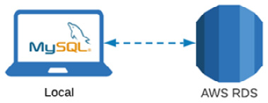
Figure 3.4 – Diagram showing that MySQL will connect to AWS RDS

Important note

Note that while this tutorial involves the creation of a database within this AWS RDS instance for the toxicity dataset, you will be able to recycle all the components for future projects and create multiple new databases without having to repeat the tutorial. Let's get started!

Installing MySQL Workbench

Of the many database design tools available, MySQL Workbench tends to be the easiest to design, implement, and use. MySQL Workbench is simply a Graphical UI (GUI) virtual database design tool developed by Oracle and allows users to create, design, manage, and interact with databases for various projects. Alternatively, MySQL can be used in the form of MySQL Shell, allowing users to interact with databases using the terminal command line. For those interested in working from the terminal command line, MySQL Shell can be downloaded by navigating to https://dev.mysql.com/downloads/shell/ and using the Microsoft Installer (MSI). However, for the purposes of this tutorial, we will be using MySQL Workbench instead for its user-friendly interface. Let's get started! Proceed as follows:

1. Getting MySQL Workbench installed on your local computer is fairly simple and easy to complete. Go ahead and navigate to https://dev.mysql.com/downloads/workbench/, select your respective operating system, and click Download, as illustrated in the following screenshot:
   

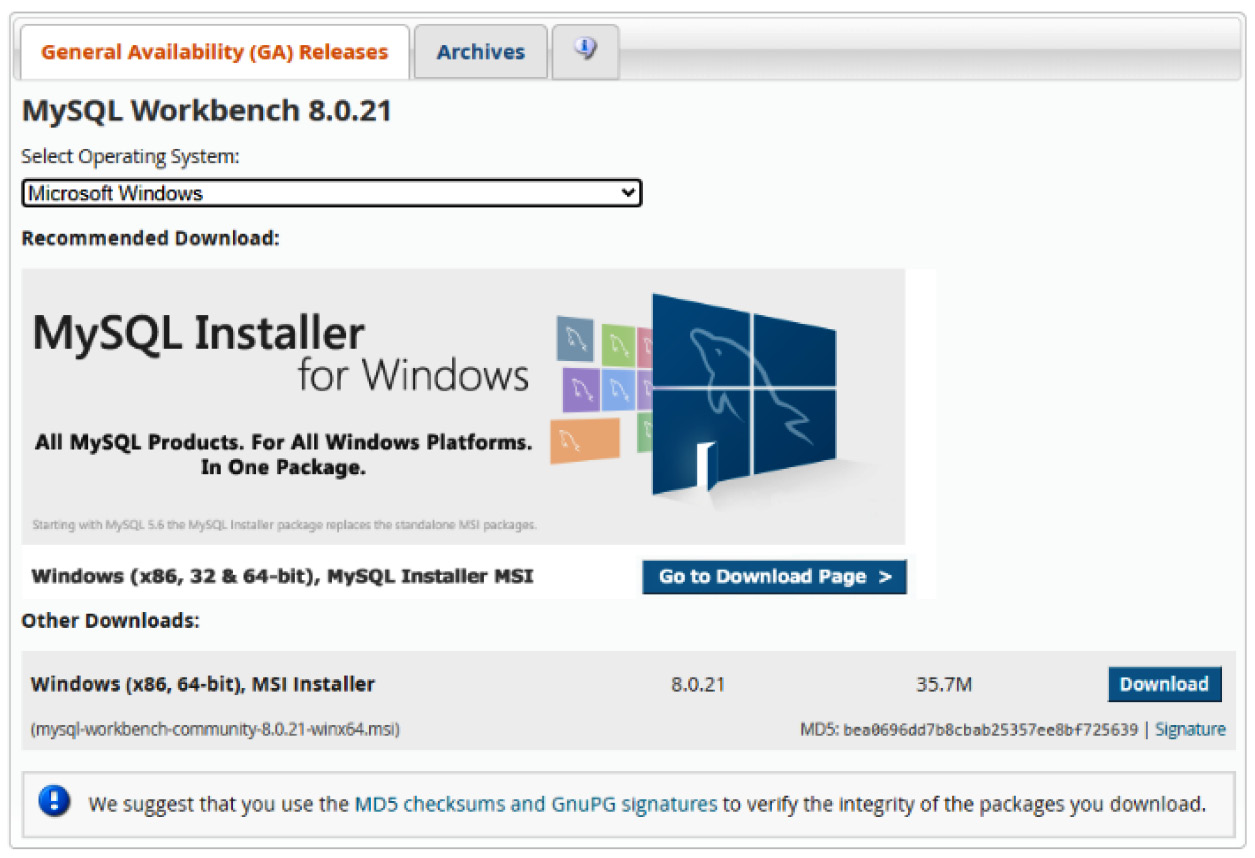
   Figure 3.5 – MySQL Installer page

2. Upon downloading the file, click Install. Follow through the installation steps if you have specific criteria that need to be met; otherwise, select all the default options. Be sure to allow MySQL to select the standard destination folder followed by the Complete setup type, as illustrated in the following screenshot:

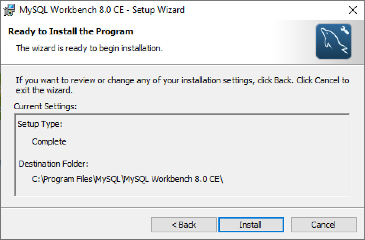
Figure 3.6 – MySQL Installer page (continued)

With that, MySQL Workbench has now been successfully installed on your local machine. We will now head to the AWS website to create a remote instance of a database for us to use. Please note that we will assume that you have already created an AWS account.

Creating a MySQL instance on AWS

Let's create a MySQL instance, as follows:

1. Navigate to https://www.aws.amazon.com and log in to your AWS account. Once logged in, head to the AWS Management Console, and select RDS from the Database section, as illustrated in the following screenshot:
   

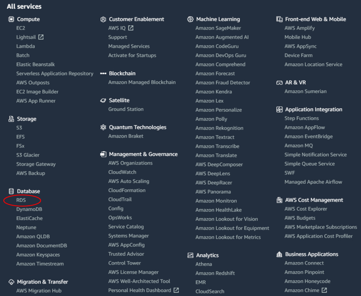
   Figure 3.7 – AWS Management Console page

2. From the top of the page, click the Create Database button. Select the Standard create option for the database creation method, and then select MySQL as the engine type, as illustrated in the following screenshot:
   

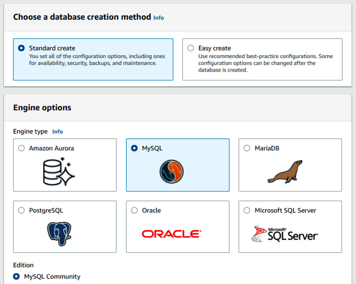
   Figure 3.8 – RDS engine options

3. In the Templates section, you will have three different options: Production, Dev/Test, and Free tier. While you can certainly select the first two options if you are planning to use a production-level server, I would recommend selecting the third option, Free tier, in order to take advantage of it being free. The following screenshot shows this option being selected:
   

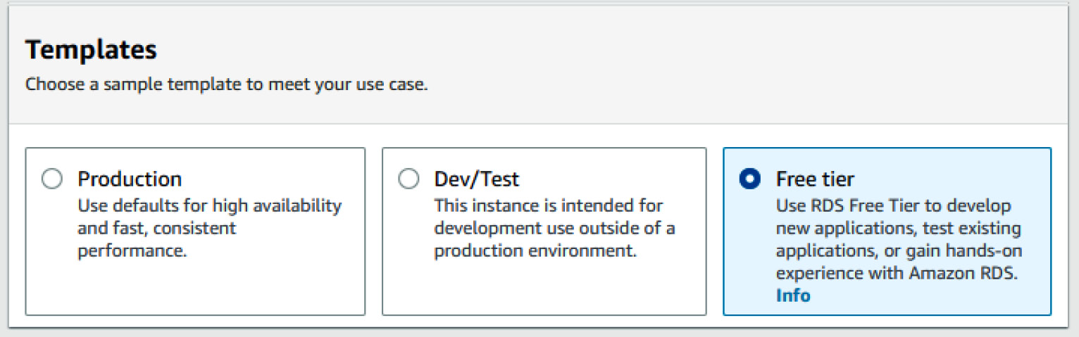
   Figure 3.9 – RDS template options

4. Under the Settings section, give the name of toxicitydatabase for the DB instance identifier field. Next, add the master username of admin, followed by a password of your choice. You may also take advantage of the Auto generate a password feature that AWS provides. If you select this option, the password will be made available to you after the instance is created. The process is illustrated in the following screenshot:
   

   Figure 3.10 – RDS settings options

5. Under the DB Instance Class section, select the Burstable Classes option followed by a db.t2.micro instance type. For storage, select the default parameters in which the Storage Type is General Purpose (SSD) option is selected, and allocate a size of 20 gigabytes (GB) for the server. Be sure to disable the autoscaling capability as we will not require this feature.
6. Finally, when it comes to connectivity, select your default Virtual Private Cloud (VPC), followed by the default subnet. Be sure to change the Public Access setting to Yes as this will allow us to connect to the instance from our local MySQL installation. Next, ensure that the Password and IAM database authentication option in the Database authentication section is selected, as illustrated in the following screenshot. Next, click Create Database:
   

   Figure 3.11 – RDS password-generation options

7. Once the database creation process is started, you will be redirected to your RDS console consisting of a list of databases where you will see a toxicitydataset database being created, as illustrated in the following screenshot. Note that the Status column of the database will show as Pending for a few moments. In the meantime, if you requested that AWS automatically generate a password for your database, you will find that in the View connection details button at the top of the page. Note that for security reasons, these credentials will never be revealed to you again. Be sure to open these details and copy all of the contents to a safe location. Connecting to this remote database via the local MySQL interface will require the master Username, the master Password, and the specified Endpoint values. With that, we have now created an AWS RDS server and we can now leave AWS in its current state and divert our full attention to MySQL Workbench:

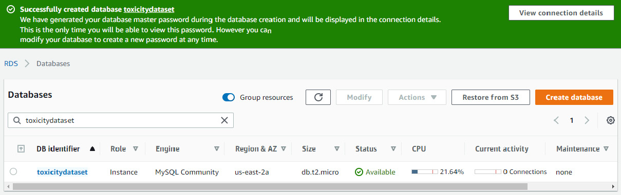
Figure 3.12 – RDS menu

With our AWS infrastructure prepared, let's go ahead and start working with our newly created database.

Working with MySQL

Once the setup on AWS is complete, go ahead and open MySQL Workbench. Note that you may be prompted to restart your computer. Follow these next steps:

1. You should be greeted with a welcome message, followed by various options. To the right of the MySQL Connections section, click the + sign to add a new connection, as illustrated in the following screenshot:
   

   Figure 3.13 – MySQL Connections button

2. In this menu, we will create a new database connection called toxicity_db_tutorial. We will select the Standard (TCP/IP) connection method. Change the Hostname field to the endpoint that was provided to you in the connection details page in AWS. Next, add the username and password that was either specified or generated for you in AWS. Be sure to store your password in the vault to access it at a later time. Finally, click on the Test Connection button. The process is illustrated in the following screenshot. If all steps were correctly followed, you should receive a Successful connection response:
   

   Figure 3.14 – MySQL Setup New Connection menu

3. In the main menu, you should see the new connection listed under the MySQL Connections section. Double-click the newly created connection, enter your root computer password (if not saved in the vault), and click OK. With that, we have created a new database connection and connected to it using MySQL Workbench.
4. The documentation for MySQL is quite extensive, as it contains a great deal of functionality that almost requires its very own book to fully cover. For the purposes of this tutorial, we will focus our efforts on a subset of functionality that is most commonly used in the data science field. There are three main sections within the MySQL Workbench window a user should be aware of—the schema navigator, the query editor, and the output window, as illustrated in the following screenshot:

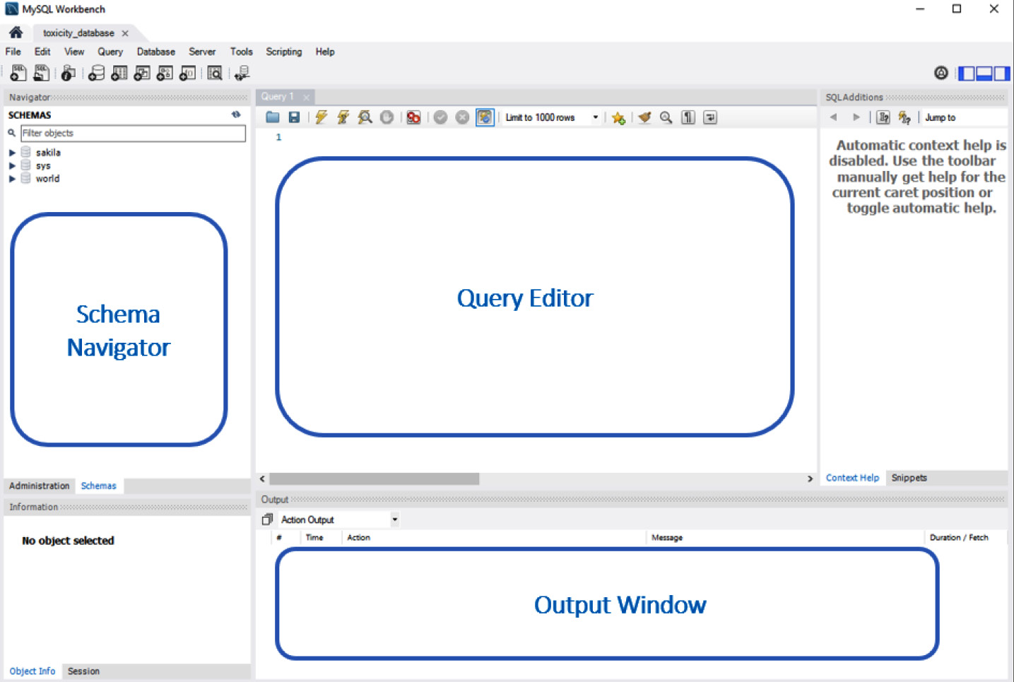
Figure 3.15 – MySQL Workbench preview

The schema navigator is the section of the window that allows users to navigate between databases. Depending on who you ask and in what context, the words schema and database are sometimes synonymous and used interchangeably. Within the context of this book, we will define schema as the blueprint of a database, and database as the database itself.

The query editor is the section of the page where you, as the user, will execute your SQL scripts. Within this section, data can be created, updated, queried, or deleted. You can use the output window, as the name suggests, for displaying the output of your executed queries. If a query goes wrong or if something unexpected happens, you will likely find an important message about it listed here.

Creating databases

Before we can begin making any queries, we will need some data to work with. Let's take a look at the currently existing databases in our new server. In the query editor, type in SHOW DATABASES;, and click on the Execute () button. You will be provided a list of databases available on your system. Most of these databases were either created from previous projects or by your system to manage data. Either way, let's avoid using those. Now, follow these next steps:

1. We can create a new database using the following SQL statement:

   CREATE DATABASE IF NOT EXISTS toxicity_db_tutorial;

2. In the output window, you should see a message confirming the successful execution of this statement. Let's now go ahead and populate our database with a previously existing CSV file. Select the Schemas tab from the schema navigator and refresh the list using the icon with two circular arrows. You will see the newly created database appear in the list, as illustrated here:
   

   Figure 3.16 – MySQL schema list

3. Next, right-click on the database, and click on Table Data Import Wizard. Navigate to and select the dataset_toxicity_sd.csv. CSV file. When prompted to select a destination, select the default parameters, allowing MySQL to create a new table called dataset_toxicity_sd within the toxicity_db_tutorial database. In the Import Configuration settings, allow MySQL to select the default datatypes for the dataset. Continue through the wizard until the import process is complete. Given the remote nature of our server, it may take a few moments to transfer the file.
4. Once the file is fully imported into AWS RDS, we are now ready to examine our data and start running a few SQL statements. If you click on the table within the schema navigator, you will see a list of all columns that were imported from the CSV file, as illustrated in the following screenshot:

Figure 3.17 – List of columns in the toxicity dataset

Taking a closer look at these columns, we notice that we begin with an ID column that is operating as our PK or UID, with the datatype int, for integer. We then notice a column called smiles, which is a text or string representing the actual chemical structure of the molecule. Next, we have a column called toxic, which is the toxicity of the compound represented as 1 for toxic, or 0 for non-toxic. We will call the toxic column our label. The rest of the columns ranging from FormalCharge to LogP are the molecules' attributes or features. One of the main objectives that we will embark upon in a later chapter is developing a predictive model to use these features as input data and attempt to predict the toxicity. For now, we will be using this dataset to explore SQL and its most common clauses and statements.

Querying data

With the file fully imported into AWS RDS, we are now ready to run a few commands.

We will begin with a simple SELECT statement in which we will retrieve all of our data from the newly created table. We can use the * argument after the SELECT command to denote all data within a particular table. The table itself can be specified at the end using the following syntax: <database_name>.<table_name>:.

In the actual command, it looks like this:

SELECT * from toxicity_db_tutorial.dataset_toxicity_sd;

This gives us the following output:

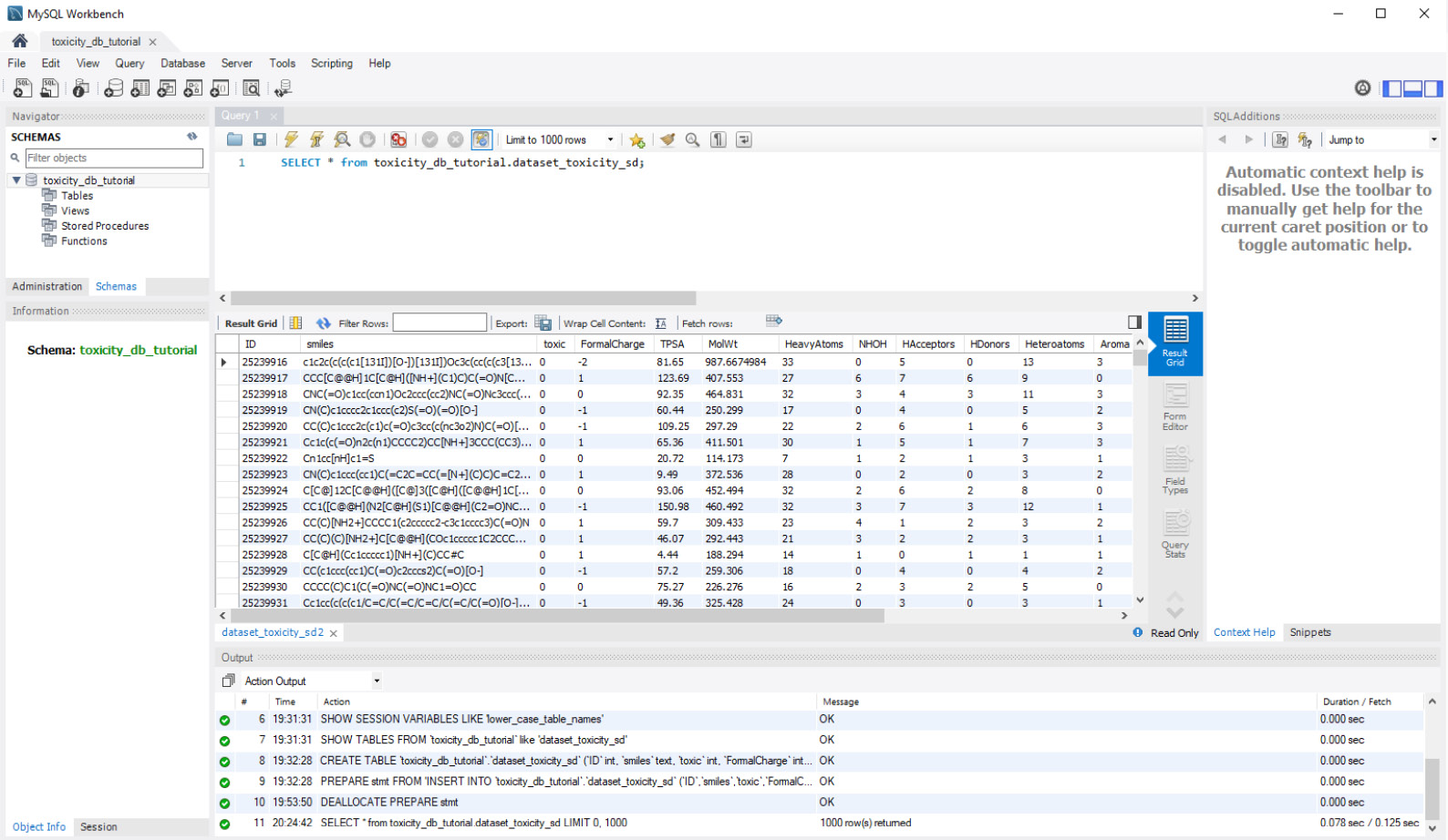
Figure 3.18 – MySQL Workbench query preview

We will rarely query all columns and all rows of our data in any given query. More often than not, we will limit the columns to those of interest. We can accomplish this by substituting the * argument with a list of columns of interest, as follows:

SELECT

  ID,

      TPSA,

      MolWt,

      LogP,

      toxic

from toxicity_db_tutorial.dataset_toxicity_sd;

Notice that the columns are separated by a comma, whereas the other arguments within the statement are not. In addition to limiting the number of columns, we can also limit the number of rows using a LIMIT clause followed by the number of rows we want to retrieve, as follows:

SELECT

  ID,

      TPSA,

      MolWt,

      LogP,

      toxic

from toxicity_db_tutorial.dataset_toxicity_sd LIMIT 10;

In addition to specifying our columns and rows, we can also apply operations to column values such as addition, subtraction, multiplication, and division. We can also filter our data based on a specific set of conditions. For example, we could run a simple query for the ID and smiles columns for all toxic compounds (toxic=1) in the database, as follows:

SELECT

  ID,

    SMILES,

     toxic

from toxicity_db_tutorial.dataset_toxicity_sd

WHERE toxic=1;

Similarly, we could also find all non-toxic compounds by changing the final line of our statement to WHERE toxic = 0 or to WHERE toxic != 1. We can extend this query with the addition of more conditionals within a WHERE clause.

Conditional querying

Conditional queries can be used to filter data more effectively, depending on the use case at hand. We can use the AND operator to query data relating to a specific toxicity and molecular weight (mol wt). Note that the AND operator would ensure that both conditions would need to be met, as illustrated in the following code snippet:

SELECT

  ID,

      SMILES,

     toxic

from toxicity_db_tutorial.dataset_toxicity_sd

WHERE toxic=1 AND MolWt > 500;

Alternatively, we can also use the OR operator in which either one of the conditions needs to be met—for example, the preceding query would require that the data has a toxic value of 1, and a mol wt of 500, thus returning 26 rows of data. The use of an OR operator here instead would require that either one of the conditions is met, thus returning 318 rows instead. Operators can also be used in combination with one another. For example, what if we wanted to query the IDs, smiles representations, and toxicities of all molecules that have 1 hydrogen acceptor, and either 1, 2, or 3 hydrogen donors? We can fulfill this query with the following statement:

SELECT

   ID,

      SMILES,

      toxic

from toxicity_db_tutorial.dataset_toxicity_sd

WHERE HAcceptors=1 AND (HDonors = 1 OR HDonors = 2 OR HDonors = 3);

It is important to note that when specifying multiple OR operators for values in consecutive order such as with the three HDonors values, the BETWEEN operator can be used instead to avoid unnecessary repetition.

Grouping data

Another common practice when running queries against a database is grouping data by a certain column. Let's take as an example a situation in which we must retrieve the total number of instances of toxic versus non-toxic compounds within our dataset. We could easily query the instances in which the values of 1 or 0 are present using a WHERE statement. However, what if the number of outcomes was 100 instead of 2? It would not be feasible to run this query 100 times, substituting the value in each iteration. For this type of operation, or any operation in which the grouping of values is of importance, we can use a GROUP BY statement in combination with a COUNT function, as illustrated in the following code snippet:

SELECT

  ID,

    SMILES,

    COUNT(*) AS count

from toxicity_db_tutorial.dataset_toxicity_sd

GROUP BY toxic

This is shown in the following screenshot:

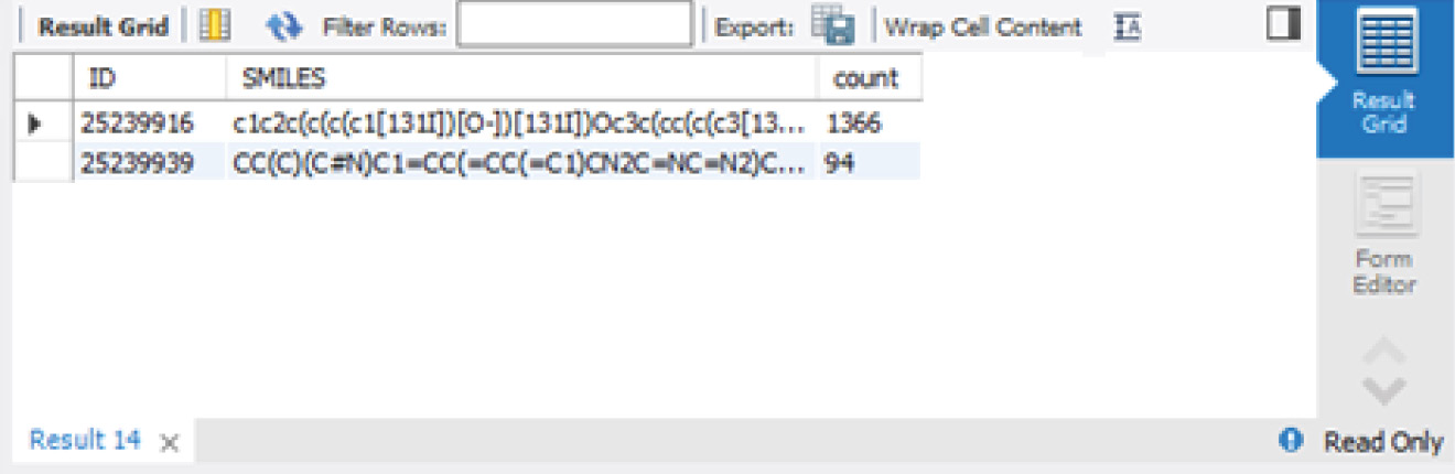
Figure 3.19 – MySQL Workbench GROUPBY preview

Now that we have explored how to group our data, let's go ahead and learn how to order it as well.

Ordering data

There will be some instances in which your data will need to be ordered in some fashion, either in an ascending or descending manner. For this, you can use an ORDER BY clause in which the sorting column is listed directly after, followed by ASC for ascending or DESC for descending. This is illustrated in the following code snippet:

SELECT

  ID,

     SMILES,

  toxic,

   ROUND(MolWt, 2) AS roundedMolWt

from toxicity_db_tutorial.dataset_toxicity_sd

ORDER BY roundedMolWt DESC

Joining tables

Often when querying records, tables will have been normalized, as previously discussed, to ensure that their data was properly stored in a relational manner. It will often be the case that you will need to merge or join two tables together to prepare your dataset of interest prior to beginning any type of meaningful Exploratory Data Analysis (EDA). For this type of operation, we can use a JOIN clause to join two tables together.

Using the same Table Data Import Wizard method for the previous dataset, go ahead and load the dataset_orderQuantities_sd.csv dataset into the same database. Recall that you can specify the same database name but a different table name within the import wizard. Once loaded, we will now have a database consisting of two tables: dataset_toxicity_sd and dataset_orderQuantities_sd.

If we run a SELECT * statement on each of the tables, we notice that the only column the two datasets have in common is the ID column. This will act as the UID to connect the two datasets. However, we also notice that the toxicity dataset consists of 1461 rows, whereas the orderQuantities dataset consists of 728 rows. This means that one dataset is missing quite a few rows. This is where different types of JOIN clauses come in.

Imagine the two datasets as circles to be represented as Venn diagrams with one circle (A) consisting of 1461 rows of data, and one circle (B) consisting of 728 rows of data. We could join the tables such that we would discard any rows that do not match using an INNER JOIN function. Notice that this is represented in the following screenshot as the intersection, or A B, of the two circles. Alternatively, we could run a LEFT JOIN or RIGHT JOIN statement to our data, neglecting the differing contents of one of the datasets represented by A' B or A B'. Finally, we can use an OUTER JOIN statement to join the data, merging the two tables regardless of missing rows, known as a union, or A B:

Figure 3.20 – Representation of the four main join methods

As you begin to explore datasets and join tables, you will find the most common JOIN clause is in fact the INNER JOIN statement, which is what we will need for our particular application. We will structure the statement as follows: we will select columns of interest, specify the source table, and then run an inner join in which we match the two ID columns together. The code is illustrated in the following snippet:

SELECT

  dataset_toxicity_sd.id,

     dataset_toxicity_sd.SMILES,

     dataset_orderQuantities_sd.quantity_g

FROM

  toxicity_db_tutorial.dataset_toxicity_sd

INNER JOIN toxicity_db_tutorial.dataset_orderQuantities_sd

  ON dataset_toxicity_sd.id = dataset_orderQuantities_sd.id

With that, we have successfully managed to take our first dataset (consisting of only the individual research and development molecules and their associated properties) and join it with another table (consisting of the order quantities of those molecules), allowing us to determine which substances we currently have in stock. Now, if we needed to find all compounds with a specific lipophilicity (logP), we can identify which ones we have in stock and in which quantities.

Summary

SQL is a powerful language when it comes to querying vast amounts of data from relational databases—a skill that will serve you well in all areas of technology and most areas of biotechnology. As most companies begin to grow their database capabilities, you will likely encounter databases of many kinds, especially relational databases.

When it comes to theory, we discussed some of the most important characteristics of relational databases and how data is generally normalized. We looked over an example of patient data and how a table could be normalized to reduce repetition when being stored. We also looked over some of the most common open source and enterprise databases available and readily used on the market today.

When it comes to applications, we put together a robust AWS RDS database server and deployed it to the cloud. We then connected our local instance of MySQL to that server and populated it with a new database using a CSV file. We then went over some of the most common SQL statements and clauses used in the industry today. We looked at ways to select, filter, group, and order data. We then looked at an example of joining two tables together and understood the different join methods available to us.

Although this book was designed to introduce you to some of the most important core concepts every data scientist should know, there were many other topics within SQL that we did not cover. I would urge you to review the MySQL documentation to learn about the many other exciting statements available, allowing you to query data in many different shapes and sizes. SQL will always be used specifically to retrieve and review data in a tabular form but will never be the proper tool to visualize data—this task is best left to Python and its many visualization libraries, which will be the focus of the next chapter.