Chapter 2: Introducing Python and the Command Line

When walking into a coffee shop, you will almost immediately notice three types of people: those socializing with others, those working on projects, and those who code. Coders can easily be spotted by the black background and white letters on their computer screens – this is known as the command line. To many, the command line can look fierce and intimidating, but to others, it is a way of life.

One of the most essential parts of conducting any type of data science project is the ability to effectively navigate directories and execute commands via the Terminal command line. The command line allows users to find files, install libraries, locate packages, access data, and execute commands in an efficient and concise way. This chapter is by no means a comprehensive overview of all the capabilities the command line has, but it does cover a general list of essential commands every data scientist should know.

In this chapter, we'll cover the following specific topics:

• Introducing the command line
• Discovering the Python language
• Tutorial – getting started in Python
• Tutorial – working with Rdkit and BioPython

Technical requirements

In this chapter, we will use the Terminal command line, which can be found in the Applications folder (macOS), or Command Prompt, which can be found in the Start menu (Windows PC). Although the two are equivalent in functionality, the syntax behind some of the commands will differ. If you are using a PC, you are encouraged to download Git for Windows (https://git-scm.com/download/win), which will allow you to follow along using the Bash command line. As we begin to edit files in the command line, we will need an editor called Vim. Most Mac users will have Vim preinstalled on their systems. PC users are encouraged to download Vim from their website (https://www.vim.org/download.php).

In addition, we will be exploring Python using the Anaconda distribution. We will go over getting this downloaded on your system soon. The process of installing Anaconda is nearly identical for both Mac and PC users, and the execution of Python code is nearly identical as well.

Throughout this book, the code you see will also be available for you on GitHub. We can think of GitHub as a space where code can live, allowing us to maintain versioning, make edits, and share our work with others. As you follow along in this chapter, you are encouraged to refer to the associated GitHub repository, which can be found at https://github.com/PacktPublishing/Machine-Learning-in-Biotechnology-and-Life-Sciences.

Introducing the command line

The command line is available for Mac, PC, and Linux. While the following examples were executed on a Mac, very similar functionality is also applicable on a PC, but with a slightly different syntax.

You can begin the process by opening the command line (known as Terminal on a Mac and Command Prompt on a PC). Opening Terminal will usually, by default, bring you to what's known as your home directory. The text you first see will specify your username and the name of your system, separated by the @ symbol. Let's look at some basic commands.

In order to identify the path of your current (working) directory, you can use the pwd command:

  $ pwd

This will return the exact directory that you are currently in. In the case of my system, the returned path was as follows:

Users/alkhalifas

In order to identify the contents within this particular directory, you can use the ls command, which will return a list of directories and files:

  $ ls

You can make a new directory within the command line by using the mkdir command, followed by the name of the directory you wish to create. For example, you can create the machine-learning-practice directory using the following command:

  $ mkdir machine-learning-biotech

If you once again list the contents within this directory using the ls command, the new directory will appear in that list. You can navigate to that directory using the cd (that is, change directory) command:

  $ cd machine-learning-practice

You can once again use the pwd command to check your new path:

  $ pwd

Users/alkhalifas/machine-learning-biotech

In order to return to the previous directory, you can use the cd command, followed by a blank space and two periods ( ..):

  $ cd ..

Important note

It is worth mentioning that depending on the command line you are using, the directory names can be case-sensitive. For example, entering Downloads instead of downloads can be interpreted as a different location, so this may return an error. Maintaining consistency in how you name files and directories will be key to your success in using the command line.

Creating and running Python scripts

Now that you've learned a few of the basics, let's go ahead and create our first Python application using the command line. We can create and edit a new file using Vim, which is a text editor. If you do not have Vim installed on your current system, you are encouraged to install it using the link provided in the Technical requirements section of this chapter. Once installed on your local machine, you can call the vim command, followed by the name of the file you wish to create and edit:

  $ vim myscript.py

This will open up an empty file within the Vim editor of your command line where you can write or paste your code. By default, you will begin in the view mode. You can change to the edit mode by pressing the I key on your keyboard. You will notice that the status at the bottom of the Vim window has changed to - - INSERT - -, which means you can now add code to this file:

Figure 2.1 – The Vim window

Type (or copy and paste) the following few lines of Python code into the file, and then click the Esc key. You will notice that the status is no longer - - INSERT - - and you can no longer edit the file. Next, type :wq and press Enter. The w key will write the file and the q key will quit the editor. For more details on other Vim commands, see the Vim website at https://www.vim.org/:

# myscript.py

import datetime

now = datetime.datetime.now()

print("Hello Biotech World")

print ("The current date and time is:")

print (now.strftime("%Y-%m-%d %H:%M:%S"))

With that, you have now written your first Python script. We can go ahead and execute this script using the Python interpreter you installed earlier. Before we do so, let's talk about what the script will do. Starting on the first line, we will import a library known as datetime, which will allow us to determine the current date and time of our system. Next, we assign the datetime object to a variable we will call now. We will discuss objects and variables in the following section, but for the time being, think of them as variables that can be filled with values such as dates or numbers. Finally, we will print a phrase that says Hello Biotech World!, followed by a statement of the current time.

Let's give this a try:

  $ python3 myscript.py

Upon executing this file, the following results will appear on your screen:

Hello Biotech World!

The current date and time is:

2021-05-23 18:40:21

In this example, we used a library called datetime, which was installed by default when you installed the Anaconda distribution. There were many others that were also installed, and many more that were not. As we progress through these projects, we will be using many of these other libraries that we can install using pip.

The previous example worked without any errors. However, this is seldom the case when it comes to programming. There will be instances in which a missing period or unclosed bracket will lead to an error. In other situations, programs will run indefinitely – perhaps in the background without your knowledge. Closing the Terminal command line generally halts running applications. However, there will be times in which closing a command-line window is not an option. To identify processes running in the background, you can use the ps (that is, process) command:

  $ ps -ef

This will display a list of all running processes. The first column, UID, is the user ID, followed by the PID (process ID) column. A few columns further to the right you can see the specific names of the files (if any) that are currently active and running. You can narrow down the list using the grep command to find all those relating to Python:

  $ ps -ef | grep python

If a Python script (for example, someScript.py) is running continuously in the background, you can easily determine the process ID by using the grep command, and this means you can subsequently kill the process with the pkill command:

  $ pkill -9 -f someScript.py

This will terminate the script and free up your computer's memory for other tasks.

Installing packages with pip

One of the best resources available to manage Python libraries is the Python Package Index (PyPI), which allows you to install, uninstall, and update libraries as needed. One of the main libraries we will be using is scikit-learn (sklearn), which we can install using the pip install command directly in the Terminal command line:

  $ pip install sklearn

The package manager will then print some feedback messages alerting you to the status of the installation. In some cases, the installation will be successful, and in others, it may not be. The feedback you receive here will be helpful in determining what next steps, if any, need to be taken.

There will be instances in which one library will require another to function – this is known as a dependency. In some cases, pip will automatically handle dependencies for you, but this will not always be the case.

To identify the dependencies of a library, you can use the pip show command:

  $ pip show sklearn

The command line will then print the name, version, URL, and many other properties associated with the given library. In some instances, the version shown will be outdated or simply not the version you need. You can either use the pip install command again to update the library to a more recent version, or you can select a specific version by specifying it after the library name:

  $ pip install sklearn==0.15.2

As the number of packages you install begins to grow, remembering the names and associated versions will become increasingly difficult. In order to generate a list of packages in a given environment, you can use the pip freeze command:

  $ pip freeze > requirements.txt

This command will freeze a list of libraries and their associated versions and then write them to a file called requirements.txt. This practice is common within teams when migrating code from one computer to another.

When things don't work…

Often, code will fail, commands will malfunction, and issues will arise for which a solution will not be immediately found. Do not let these instances discourage you. As you begin to explore the command line, Python, and most other code-based endeavors, you will likely run into errors and problems that you will not be able to solve. However, it is likely that others have already solved your problem. One of the best resources available for searching and diagnosing code-related issues is Stack Overflow – a major collaboration and knowledge-sharing platform for individuals and companies to ask questions and find solutions for problems relating to all types of code. It is highly encouraged that you take advantage of this wonderful resource.

Now that we've had a good look at the command line and its endless capabilities, let's begin to explore Python in more detail.

Discovering the Python language

There are many different computer languages that exist in the world today. Python, R, SQL, Java, JavaScript, C++, C, and C# are just a few examples. Although each of these languages is different when it comes to their syntax and application, they can be divided into two general categories: low-level and high-level languages. Low-level languages – such as C and C++ – are computer languages operating at the machine level. They concern themselves with very specific tasks, such as the movement of bits from one location to another. On the other hand, high-level languages – such as R and Python – concern themselves with more abstract processes such as squaring numbers in a list. They completely disregard what is happening at the machine level.

Before we discuss Python in more detail, let's talk about the idea of compiling programs. Most programs – such as programs written in C++ and Java – require what is known as a compiler. Think of a compiler as a piece of software that converts human-readable code into machine-readable code immediately before the program is started or executed. While compilers are required for most languages, they are not required for languages such as Python. Python requires what is known as an interpreter, which is inherently similar to a compiler in structure, but it executes commands immediately instead of translating them to machine-readable code. With that in mind, we will define Python as a high-level, general-purpose, and interpreted programming language. Python is commonly used for statistical work, machine learning applications, and even game and website development. Since Python is an interpreted language, it can either be used within an IDE or directly within the Terminal command line:

  $ python

Next, we'll talk about IDEs.

Selecting an IDE

Python code can be prepared in several different ways. For instance, we could prepare it through the Terminal command line using the Vim text editor, as demonstrated in the previous section. While this method works quite well, you will commonly encounter redundancy when it comes to structuring files, organizing directories, and executing code. Alternatively, most data scientists default to more graphical editors known as Integrated Development Environments (IDEs). There are numerous IDEs that are free and available to download, such as Spyder, PyCharm, Visual Studio, or Jupyter Lab.

Each IDE has its respective advantages and disadvantages, and those are highly dependent on the use cases and workstreams of the user. Most new data scientists generally default to Jupyter Notebook and/or Jupyter Lab when getting started. For the purposes of this book, all code will be prepared and shared using Jupyter Notebook. Assuming the installation instructions for Anaconda were properly followed in the previous chapter, Jupyter Notebook should already be installed on your local machine. You can start the application by opening Anaconda Navigator and selecting Jupyter Notebook:

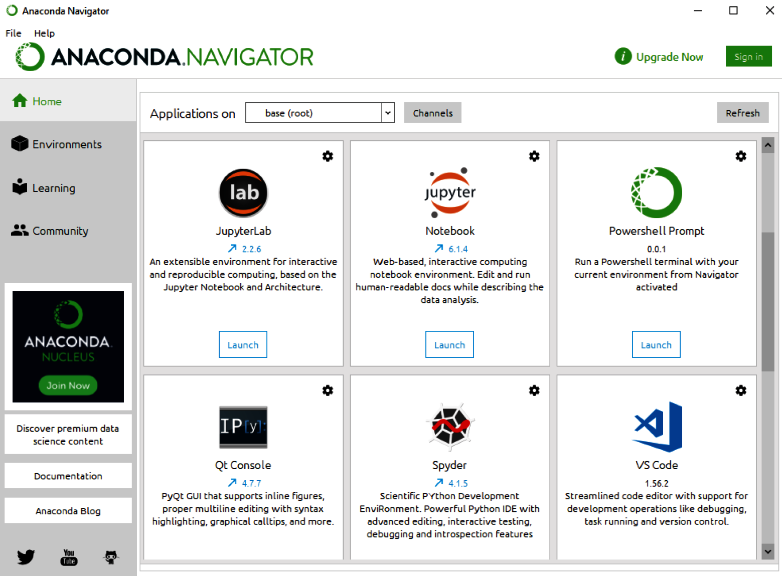
Figure 2.2 – The Anaconda Navigator window

Alternatively, you can also start the Jupyter Notebook application using the Terminal command line by typing in the following command:

  $ jupyter notebook

Upon hitting enter, the same Jupyter Notebook application we saw previously should appear on your screen. This is simply a faster method of opening Jupyter Notebook.

Data types

There are many different types of data that Python is capable of handling. These can generally be divided into two main categories: primitives and collections, as illustrated in the following diagram:

Figure 2.3 – A diagram showing Python data types

The first data type category is primitive values. As the name implies, these data types are the most basic building blocks in Python. A few examples of these include the following:

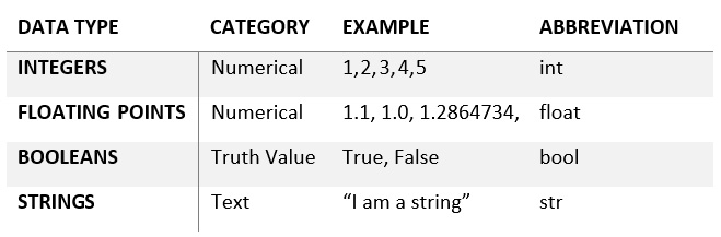
Figure 2.4 – A table of primitive data types

The second data type category is collections. Collections are made up of one or more primitive values put together. Each type of collection has specific properties associated with it, yielding distinct advantages and disadvantages in certain conditions. A few examples of these include the following:

Figure 2.5 – A table showing different kinds of data type collections

As scientists, we are naturally inclined to organize information as best we can. We previously classified data types based on their primitive and collective nature. However, we can also classify data types based on a concept known as mutability. Mutability can also be thought of as delete-ability. Variables, such as those representing a list, hold an instance of that type. When the object is created or instantiated, it is assigned a unique ID. Normally, the type of this object cannot be changed after it is defined at runtime, however, it can be changed if it is considered mutable. Objects such as integers, floats, and Booleans are considered immutable and therefore cannot be changed after being created. On the other hand, objects such as lists, dictionaries, and sets are mutable objects and can be changed. Therefore, they are considered mutable, as you can see from Figure 2.6:

Figure 2.6 – Python data types according to their mutability

Now that we have taken a look at some of the basics, let's explore some of the more exciting areas of the Python language.

Tutorial – getting started in Python

Python is an extensive language, and any attempt to summarize its capabilities in under 10 pages would be limited. While this book is not intended to be used as a comprehensive guide to Python, we will talk through a number of the must-know commands and capabilities that every data scientist should be aware of. We will see the vast majority of these commands come up in the tutorials to come.

Creating variables

One of the core concepts in Python is the idea of variables. Variables are items that Python manipulates, with each variable having a type. Operators such as addition (+) or subtraction (-) can be combined with variables to create expressions. An example of an expression can be created using three variables. First, a value of 5 will be assigned to the x variable, and then, a value of 10 will be assigned to the y variable. The two variables (x and y), which are now representing numerical values, are considered objects in Python. A new variable, z, can be created to represent the sum of x and y:

     $ python

  >>> x = 5

  >>> y = 10

  >>> z = x + y

  >>> print(z)

  15

Variables can take on many data types. In addition to the integer values shown in the preceding code, variables can be assigned strings, floats, or even Booleans:

  >>> x = "biotechnology"

  >>> x = 3.14159

  >>> x = True

The specific data type of a variable can be determined using the type() function:

  >>> x = 55

  >>> type(x)

      int

Data types do not need to be explicitly declared in Python (unlike other languages such as C++ or Java). In fact, Python also allows variables to be cast into other types. For example, we can cast an integer into a string:

  >>> x = 55

  >>> x = str(x)

  >>> type(x)

      str

We can see from what was returned that the data is now of the string type!

Importing installed libraries

After a library has been installed, you can import the library into your Python script or Jupyter Notebook using the import function. You can import the library as a whole in the following way:

>>> import statistics

Alternatively, we can explicitly import all classes from the library:

>>> from statistics import *

The best way to import any library is to only import the classes that you plan to use. We can think of classes as standalone parts of a given library. If you plan to calculate the mean of a series of numbers, you can explicitly import the mean class from the statistics library:

>>> from statistics import mean

Installing and importing libraries will become second nature to you as you venture further into the data science field. The following table shows some of the most common and most useful libraries any new data scientist should know. Although not all of these will be covered within the scope of this book, they are useful to know.

Figure 2.7 – A table showing some of the most common Python libraries

The libraries included in the previous table are some of the most common ones you will face as you begin your journey in the data science space. In the following section, we will focus on the math library to run a few calculations.

General calculations

Within the Python language, we can create variables and assign them specific values, as we previously observed. Following this, we can use the values within these variables to form expressions and conduct mathematical calculations. For example, take the Arrhenius equation, commonly used for forecasting molecular stability and calculating the temperature dependence of reaction rates. This equation is commonly used in R&D for two main purposes:

• Optimizing reaction conditions to maximize yields within a synthetic manufacturing process
• Predicting the long-term stability of tablets and pills given changes in temperature and humidity

The equation can be expressed as follows:

In this case, k is the rate constant, A is the frequency factor, EA is the activation energy, R is the ideal gas constant, and T is the temperature in Kelvin (K). We can use this equation to calculate how a change in temperature would affect the rate constant. Let's assume that the current need is to predict what would happen if the temperature changed from 293 K to 303 K. First, we would need to define some variables:

     >>> from math import exp

     >>> EA = 50000

     >>> R = 8.31

     >>> T1 = 293

  

     >>> exp(-EA / (R*T1))

  1.2067e-09

We can now reassign the temperature variable another value and recalculate:

     >>> T2 = 303

     >>> exp(-EA / (R*T2))

  2.3766e-09

In conclusion, this shows that a simple change in temperature nearly doubles the faction!

Lists and dictionaries

Lists and dictionaries are two of the most common and fundamental data types in Python. Lists are simply ordered collections of elements (similar to arrays) and can hold elements of the same type, or of different types:

  >>> homogenousList = ["toluene", "methanol", "ethanol"]

  >>> heterogenousList = ["dichloromethane", 3.14, True]

The length of any given list can be captured using the len() function:

  >>> len(heterogenousList)

  3

List elements can be retrieved using their index location. Remember that all indexes in Python begin at 0, therefore, the first element of this list would be at the 0 index:

  >>> heterogenousList[0]

  dichloromethane

  >>> heterogenousList[1]

  3.14

Unlike their primitive counterparts, lists are mutable, as they can be altered after their creation. We can add another element to a list using the append() function:

  >>> len(homogenousList)

  3

  >>> homogenousList.append("acetonitrile")

  >>> len(homogenousList)

  4

Dictionaries, on the other hand, are often used for their association of keys and values. Given a dictionary, you can specify the name of a key along with its corresponding value. For example, a chemical inventory list containing chemical names and their expiration dates would not work well within a standard Python list. The chemical names and their dates cannot be associated together very easily in this formation.

However, a dictionary would be a perfect way to make this association:

  >>> singleChemical = {"name" : "acetonitrile",

          "exp_date" : "5/26/2021"}

This dictionary now represents the elements of a single chemical, in the sense that there is a key assigned to it for a name, and another for an expiration date. You can retrieve a specific value within a dictionary by specifying the key:

>>> singleChemical["name"]

  acetonitrile

To construct a full inventory of chemicals, you would need to create multiple dictionaries, one for each chemical, and add them all to a single list. This format is known as JSON, which we will explore in more detail later in this chapter.

Arrays

Arrays in Python are analogous to lists in the sense that they can contain elements of different types, they can have multiple duplicates, and they can be changed and mutated over time. Arrays can be easily extended, appended, cleared, copied, counted, indexed, reversed, or sorted using simple functions. Take the following as an example:

1. Let's go ahead and create an array using numpy:

   import numpy as np

   newArray = np.array([1,2,3,4,5,6,7,8,9,10])

2. You can add another element to the end of the list using the append() function:

     >>> newArray= np.append(newArray,25)

     >>> newArray

      [1,2,3,4,5,6,7,8,9,10,25]

3. The length of the array can be determined using the len() function:

     >>> len(newArray)

      11

4. The array can also be sliced using brackets and assigned to new variables. For example, the following code takes the first five elements of the list:

     >>> firstHalf = newArray[:5]

     >>> firstHalf

      [1,2,3,4,5]

Now that we have mastered some of the basics when it comes to Python, let's dive into the more complex topic of functions.

Creating functions

A function in Python is a way to organize code and isolate processes, allowing you to define an explicit input and an explicit output. Take, for example, a function that squares numbers:

def squaring_function(x):

  # A function that squares the input

  return x * x

Functions are first class in the sense that they can be assigned to variables or subsequently passed to other functions:

  >>> num = squaring_function(5)

  >>> print(num)

  25

Depending on their purpose, functions can have multiple inputs and outputs. It is generally accepted that a function should serve one specific purpose and nothing more.

Iteration and loops

There will be many instances where a task must be conducted in a repetitive or iterative manner. In the previous example, a single value was squared, however, what if there were 10 values that needed to be squared? You could either manually run this function over and over, or you could iterate it with a loop. There are two main types of loops: for loops and while loops. A for loop is generally used when the number of iterations is known. On the other hand, a while loop is generally used when a loop needs to be broken based on a given condition. Let's take a look at an example of a for loop:

input_list = [1, 2, 3, 4, 5, 6, 7, 8, 9, 10]

output_list = []

for val in input_list:

    squared_val = squaring_function(val)

    output_list.append(squared_val)

    print(val, " squared is: ", squared_val)

First, a list of values is defined. An empty list – where the squared values will be written to – is then created. We then iterate over the list, square the value, append (add) it to the new list, and then print the value. Although for loops are great for iterating, they can be incredibly slow in some cases when handling larger datasets.

However, while loops can also be used for various types of iterations, specifically when the iteration is to cease when a condition is met. Let's take a look at an example of a while loop:

current_val = 0

while current_val < 10:

    print(current_val)

    current_val += 1

Now that we have gained a stronger understanding of loops and how they can be used, let's explore a more advanced form of iteration known as list comprehension.

List comprehension

Like for loops, list comprehension allows the iteration of a process using a powerful single line of code. We can replicate the previous example of squaring values using this single line:

   >>> my_squared_list = [squaring_function(val) for val in  input_list]

There are three main reasons why you should use list comprehension:

• It can reduce several lines of code down to a single line, making your code much neater.
• It can be significantly faster than its for loop counterparts.
• It is an excellent interview question about writing efficient code. Hint hint.

DataFrames

DataFrames using the pandas library are arguably among the most common objects within the Python data science space. DataFrames are analogous to structured tables (think of an Excel spreadsheet), allowing users to structure data in rows and columns. DataFrames can be constructed using lists, dictionaries, or even full CSV documents from your local computer. A DataFrame object can be constructed as follows:

>>> import pandas as pd

>>>

df = pd.DataFrame([[1,2,3],[4,5,6],[7,8,9]],columns = ['col1','col2', 'col3'])

>>> print(df)

This will give the following output:

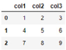
Figure 2.8 – A table showing the results of the DataFrame object

Almost every parameter within a DataFrame object can be changed and altered to fit the data within it. For example, the columns can be relabeled with full words:

>>> df.columns = ["ColumnA", "ColumnB", "ColumnC"]

New columns can be created representing an output of a mathematical function. For example, a column representing the squared values of ColumnC can be prepared:

>>> df["ColumnC_Squared"] = df["ColumnC"] ** 2

>>> print(df)

The output of this is as follows:

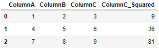
Figure 2.9 – A table showing the results of the DataFrame object

Alternatively, DataFrames can be prepared using a pre-existing CSV file from your local machine. This can be accomplished using the read_csv() function:

  >>> import pandas as pd

  >>> df = pd.read_csv('dataset_lipophilicity_sd.csv')

Instead of importing the entire dataset, a specific set of columns can be selected:

  >>> df = df[["ID", "TPSA", "MolWt", "LogP"]]

  >>> df.head()

The output of this is as follows:

Figure 2.10 – A table showing the results of the DataFrame object

Alternatively, the tail() function can also be used to view the last few rows of data:

  >>> df.tail()

DataFrames are some of the most common forms of data handling and presentation within Python, as they resemble standard 2D tables that most people are familiar with. A more efficient alternative for handling larger quantities of data is to use Apache Spark DataFrames, which can be used with the PySpark library.

Now that we are able to manage and process data locally on our machines, let's take a look at how we could retrieve data from external sources using API requests.

API requests and JSON

In some instances, data will not be available locally on your computer and you will need to retrieve it from a remote location. One of the most common ways to send and receive data is in the form of an application programming interface (API). The main idea behind an API is to use HTTP requests to obtain data, commonly communicated in the JSON format. Let's take a look at an example:

import requests

r = requests.get('https://raw.githubusercontent.com/alkhalifas/node-api-books/master/services/books.json')

data = r.json()

Think of a JSON as a list of dictionaries in which each dictionary is an element. We can select specific elements in the list based on their index locations. In Python, we begin the count at 0, therefore, the first item in our list of dictionaries will have the index location of 0:

  >>> data[0]

This gives us the following:

Figure 2.11 – A sample of the results obtained from an HTTP request

The values within the dictionary can be accessed using their corresponding keys:

  >>> data[0]["type"]

  HARD_COVER

In a similar way to CSV files, JSON files can also be imported into DataFrames using the read_json() function.

Parsing PDFs

Unlike the many structured forms of data we have imported into Python, such as CSV and JSON files, you will often encounter data in its unstructured form – for example, text files or PDFs. For most applications that use natural language processing (NLP), data is generally gathered in its unstructured form and then preprocessed into a more structured state. PDF documents are among the most common sources of text-based data and there are numerous libraries available allowing users to parse their contents more easily. Here, we will explore a new library known as tika – one of the most popular in the open source community. We can begin by installing the library using pip:

  alkhalifas@titanium ~ % pip install tika

We can then go ahead and read the specific PDF file of interest:

  from tika import parser

  raw = parser.from_file("./datasets/COVID19-CDC.pdf")

  print(raw['content'])

The data within raw['content'] will be the text of the PDF file parsed by the tika library. This data is now ready to be used and preprocessed in a subsequent NLP application.

Pickling files

The vast majority of the documents we have handled so far are files that are commonly saved locally to your computer – for example, PDFs, CSVs, and JSON files. So, how do we save a Python object? If you have an important list of items you wish to save – perhaps the chemicals from our previous example – you will need a way to save those files locally to use at a later time. For this, most data scientists use pickle. The pickle library allows you to save and store Python objects for use at a later time in the form of .pkl files. These files can later be imported back to Python and used for new tasks. This is a process known as serializing and deserializing objects in Python. Let's take a look at an example of using a .pkl file. We start by importing the pickle library and then creating a list of items:

>>> import pickle

>>> cell_lines = ["COS", "MDCK", "L6", "HeLa", "H1", "H9"]

In order to save the list as a .pkl file, we will need to specify a location for the file to be saved in. Note that we will be using the wb mode (that is, the write binary mode). We will then use the dump() function to save the contents:

>>> pickledList = open('./tmp/cellLineList.pkl', 'wb')

>>> pickle.dump(cell_lines, pickledList)

Whether the file was saved locally or shared with a colleague, it can subsequently be loaded back into Python using the load() command in a similar manner:

>>> pickledList = open('./tmp/cellLineList.pkl', 'rb')

>>> cell_lines_loaded = pickle.load(pickledList)

>>> print(cell_lines_loaded)

["COS", "MDCK", "L6", "HeLa", "H1", "H9"]

Notice that in the preceding example, we switched between two arguments – wb (write binary) and rb (read binary) – depending on the task. These are two modes that can be selected to load and save files. There are a number of other options that can be used. The main distinction that should be noted here is the use of binary formats. On Windows, opening the files in binary mode will address end-of-line characters in text files mostly seen in ASCII files. The following table provides an overview of some of the most common modes:

Figure 2.12 – A table showing the most common read/write modes

Now that we have gained a basic understanding of APIs and the operations we can perform on data, let's take a look at the use of object-oriented programming (OOP) as it relates to Python.

Object-oriented programming

Similar to many other languages – such as C++, Java, and C# – the concept of OOP can also be used in Python. In OOP, the main aim is to use classes to organize and encapsulate data objects and their associated functions.

Let's explore an example of OOP in the context of chemical inventory management. Most modern biotechnology companies have extensive inventory systems that monitor their stock of in-house chemicals. Inventory systems allow companies to ensure that supplies do not run out and expiration dates are adequately monitored, along with many other tasks. Now, we will use our current knowledge of Python alongside the concept of OOP to construct an inventory management system:

1. We begin by importing two libraries we will need to manage our dates:

   import datetime

   from dateutil import parser

2. Next, we define a name for the class using the following syntax:

   class Chemical:

3. We then construct a portion of code known as the constructor:

   class Chemical:

           def __init__(self, name, symbol, exp_date, count):

               self.name = name

               self.symbol = symbol

               self.exp_date = exp_date

               self.count = count

   The purpose of the constructor is to act as a general blueprint of the objects we intend to create. In our case, the object will be a chemical object, and each chemical object will consist of a number of parameters. In this case, the chemical has a name, a symbol, an expiration date, and a count. We use the __init__ function to initialize or create this object, and we use self to refer to that specific instance of a class. For example, if we created two chemical objects, self.name could be acetonitrile for one object and methanol for another.

4. Next, we can define a few functions that are relevant to our class. These functions are class-specific and are tied to the class in such a way that they can only be accessed through it. We call these functions member functions. Within each function, we add self as an argument to tie the function to the specific instance of interest. In the following example, we will create an isExpired() function that will read the expiration date of the chemical and return a True value if expired. We begin by determining today's date, and then retrieve the object's date using the self.exp_date argument. We then return a Boolean value that is the product of a comparison between the two dates:

           def isExpired(self):

               todays_date = datetime.datetime.today()

               exp_date = parser.parse(self.exp_date)

               return todays_date > exp_date

5. We can test this out by creating a new object using the Chemical class:

   >>> chem1 = Chemical(name="Toluene", symbol="TOL", exp_date="2019-05-20", count = 5)

6. With that, we have constructed a chemical object we call chem1. We can retrieve the fields or attributes of chem1 by specifying the name of the field:

   >>> Print(chem1.name)

   Toluene

   Notice that the name field was not followed by parentheses in the way we have previously seen. This is because name is only a field that is associated with the class and not a function.

7. We can use our function by specifying in a similar manner:

   >>> print(chem1.isExpired())

   True

   Notice that the function was followed by parentheses, however, no argument was added within it, despite the fact that the function itself within the class specifically contained the self argument.

8. We can create many instances of our class, with each instance containing a different date:

   >>> chem2 = Chemical(name="Toluene", symbol="TOL", exp_date="2021-11-25", count = 4)

   >>> chem3 = Chemical(name="Dichloromethane", symbol="DCM", exp_date="2020-05-13", count = 12)

   >>> chem4 = Chemical(name="Methanol", symbol="MET", exp_date="2021-01-13", count = 5)

   Each of these objects will return their respective values when followed by either their fields or functions.

9. We can also create functions to summarize the data within a particular instance of an object:

           def summarizer(self):

               print("The chemical", self.name, "with the symbol (",self.symbol,") has the expiration date", self.exp_date)

10. We can then call the summarizer() function on any of the chemical objects we have created in order to retrieve a human-readable summary of its status:

    >>> print(chem1.summarizer())

    The chemical Toluene with the symbol ( TOL ) has the expiration date 2019-05-20

11. The functions we have written so far have not taken any additional arguments and have simply retrieved data for us. Chemical inventory systems often need to be updated to reflect items that have expired or been consumed, thereby altering the count. Functions can also be used to change or alter the data within an object:

            def setCount(self, value):

                self.count = value

12. We can simply add value as an argument to set that instance's count (represented by self.count) to the corresponding value. We can test this using one of our objects:

    >>> chem1 = Chemical(name="Toluene", symbol="TOL", exp_date="2019-05-20", count = 5)

    >>> chem1.count

      5

    >>> chem1.setCount(25)

    >>> chem1.count

    25

There are many other uses, applications, and patterns for OOP that go above and beyond the example we have just seen. For example, inventory systems would not only need to maintain their inventories, but they would also need to manage the expiry dates of each item, record sales details, and have methods and functions to compile and report these metrics. If you are interested in the development of classes within Python, please visit the official Python documentation to learn more (https://docs.python.org/3/tutorial/classes.html).

Tutorial – working with Rdkit and BioPython

In the previous tutorial, we saw various examples of how Python can be used to calculate properties, organize data, parse files, and much more. In addition to the libraries we have worked with thus far, there are two others in particular we need to pay close attention to when operating in the fields of Biotechnology and Life Sciences: Rdkit, and BioPython. In the following sections, we will look at a few examples of the many capabilities available in these packages. With this in mind, let us go ahead and get started!

Working with Small Molecules and Rdkit

One of the most common packages data scientists use when handling data relating to small molecules is known as rdkit. Rdkit is an open-source cheminformatics and machine learning package with numerous useful functionalities for both predictive and generative purposes. The rdkit package includes many different tools and capabilities to the point that we would need a completely second book to cover in total. Highlighted below are five of the most common applications this package is generally known for, as seen in Figure 2.13:

Figure 2.13 – Some of the main functionality in the rdkit package

Let us go ahead and example a few of these capabilities in order to introduce ourselves to the rdkit package.

Working with SMILES Representations

Similar to some of the packages we have seen already, rdkit is organized by classes. Let us now take advantage of the Chem class to load a SMILES representation in a few simple steps.

We will start off by importing the Chem class:

from rdkit import Chem

One of the easiest and most common ways to transfer 2D molecular structures from one Python script to another is by using a SMILES representation. For example, we can describe a Quaternary Ammonium Compound (QAC) using its SMILES representation as seen here:

SMILES = "[Br-].[Br-].CCCCCCCCCCC[N+]1=CC=C(CCCC2=CC=[N+](CCCCCCCCCCC)C=C2)C=C1"

We can use the MolFromSmiles function within the Chem class to load our SMILES representation into rdkit:

molecule = Chem.MolFromSmiles(SMILES)

molecule

Upon printing the molecule variable we assigned above, a figure of the molecule will be returned as shown in Figure 2.14:

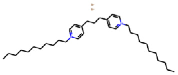
Figure 2.14 – A 2D representation of the QAC using rdkit

Notice that we did not need any additional packages to print this figure as rdkit is quire comprehensive and has everything you need to run these visualizations. In the following section, we will see another example of rdkit as it comes to similarity calculations.

With the structure now loaded, there are many different applications and calculations one can do. One of the most common methods to do here is searching for substructures within the molecule. We can accomplish this by using the MolFromSmarts function within rdkit:

tail_pattern = Chem.MolFromSmarts('CCCCCCCCCCC')

patter

Upon executing this, we yield the following figure showing the substructure of interest:

Figure 2.15 – A 2D substructure of interest

With the main molecule of interest and the pattern now both loaded, we can use the HasSubstructMatch function to determine if the substructure exists:

molecule.HasSubstructMatch(tail_pattern)

Upon executing this code, the value of True will be returned indicating that the structure does exist. On the other hand, if another substructure such as a phenol were to be run, the value would return as False, since that substructure does not exist in the main molecule.

In addition, similarity calculations can be run using the DataStructs class within rdkit. We can being by importing the class, and entering two molecules of interest:

from rdkit import DataStructs

from rdkit.Chem import Draw

mol_sim = [Chem.MolFromSmiles('[Br-].[Br-].CCCCCC[N+]1=CC=C(CCCC2=CC=[N+](CCCCCC)C=C2)C=C1'), Chem.MolFromSmiles('[Br-].[Br-].CCCCCCCCCCC[N+]1=CC=C(CCCC2=CC=[N+](CCCCCCCCCCC)C=C2)C=C1')]

If we compared the two molecules visually using the MolFromSmiles method we saw previously, we can see that there exists a minor difference between the two structures, being the double bonds in the hydrophobic tails in one of the molecules.

Next, we can use the RDKFingerprint function to calculate the fingerprints:

fps = [Chem.RDKFingerprint(x) for x in mol_sim]

Finally, we can use CosineSimilarity metric to calculate how different the two structures are:

DataStructs.FingerprintSimilarity(fps[0],fps[1], metric=DataStructs.CosineSimilarity)

This calculation will yield a value of approximately 99.14%, indicating that the structures are mostly the same with the exception of a minor difference.

Summary

Python is a powerful language that will serve you well, regardless of your area of expertise. In this chapter, we discussed some of the most important concepts when working with the command line, such as creating directories, installing packages, and creating and editing Python scripts. We also discussed the Python programming language quite extensively. We reviewed some of the most commonly used IDEs, general data types, and calculations. We also reviewed some of the more complex data types such as lists, DataFrames, and JSON files. We also looked over the basics of APIs and making HTTP requests, and we introduced OOP with regard to Python classes. All of the examples we explored in this chapter relate to applications commonly discussed within the field of data science, so having a strong understanding of them will be very beneficial.

Although this chapter was designed to introduce you to some of the most important concepts in data science (such as variables, lists, JSON files, and dictionaries), we were not able to cover them all. There are many other topics, such as tuples, sets, counters, sorting, regular expressions, and many facets of OOP that we have not discussed. The documentation for Python – both in print and online – is extensive and mostly free. I would urge you to take advantage of these resources and learn as much as you can from them.

Within this chapter, we discussed many ways to handle small amounts of data when it comes to slicing it around and running basic calculations. At the enterprise level, data generally comes in significantly larger quantities, and therefore, we'll need the right tool to tackle it. That tool is Structured Query Language (SQL), and we will get acquainted with this in the next chapter.