
Chapter 17
Using Google TensorFlow with Amazon SageMaker
WHAT'S IN THIS CHAPTER
- Introduction to Google TensorFlow
- Create a linear regression model with Google TensorFlow
- Introduction to artificial neural networks
- Create a neural network classifier with the Google TensorFlow Estimators API
- Train and deploy Google TensorFlow models on Amazon SageMaker
In the previous chapter you learned to use Amazon SageMaker to build and deploy machine learning models that were based on Amazon SageMaker's built-in implementation of popular machine learning algorithms, and models created with Scikit-learn. In this chapter you will learn to create models using Google TensorFlow and use Amazon SageMaker to train and deploy these models.
- NOTE Amazon SageMaker is only free for the first two months after you have signed up for a free-tier AWS account. After that period, you will be charged for compute resources.
- NOTE To follow along with this chapter, ensure you have created the S3 buckets listed in Appendix B.
You can download the code files for this chapter from
www.wiley.com/go/machinelearningawscloudor from GitHub using the following URL:
Introduction to Google TensorFlow
TensorFlow is a machine learning library created by Google, which was initially developed by the team at Google Brain for internal use and then subsequently released as an open source project under the Apache license in November 2015. TensorFlow requires you to model your computation problem as a tree-like structure called a computation graph, made up of nodes and leaves. The nodes of the graph represent mathematical operations or functions, and the leaf nodes represent some kind of input into the operations. The data on which this graph operates is represented as n-dimensional matrices called tensors. You can think of a tensor as a generalization of vectors and matrices.
Operation nodes are also called op nodes, and while most of them take tensors as inputs and return a tensor that represents the result of the operation, some operation nodes do not return anything. These nodes that do not return any outputs usually modify the data in the entire graph in some way, such as initializing all variables with values wherever in the graph they may be.
Leaf nodes can be of three different types:
- Constant: A constant leaf node (also known as a constant tensor) is a tensor whose value cannot be changed once it has been assigned. A constant tensor is created using the
tf.constant()Python function. You can learn more about creating constant tensors athttps://www.tensorflow.org/api_docs/python/tf/constant. - Variable: A variable leaf node (also known as a variable tensor) is a tensor whose value can be changed as the program executes. When building machine learning models, the parameters of the model such as weights and bias terms are represented using variable tensors. Variable tensors are instances of the
tf.Variableclass and can be created by either using the class constructor or thetf.get_variable()function. You can learn more about variable tensors athttps://www.tensorflow.org/api_docs/python/tf/Variable. - Placeholder: A placeholder leaf node (also known as a placeholder tensor) is a special node whose value is a tensor that you must feed into the graph when you evaluate the graph. Placeholders for tensors are typically used to feed training data and labels into your program and are created using the
tf.placeholder()function. You can learn more about tensor placeholders athttps://www.tensorflow.org/api_docs/python/tf/placeholder.
The process of running the TensorFlow program amounts to evaluating the computation graph in an object called a session. The graph is then evaluated in a session, and during the evaluation process, input data (tensors) are fed into the leaf nodes of the graph and flow through the graph toward the root node—hence the name TensorFlow. A TensorFlow session takes care of converting the computation graph into executable code and executing the graph on the CPU or GPU. The scope of the variables, constants, and tensor placeholders is restricted to the session. You can have multiple sessions with different computation graphs in each.
While this graph-based approach may seem like overkill for a simple arithmetic problem, it is extremely useful (and natural) if the computation problem that you are trying to represent is inherently graph-based, such as an artificial neural network (ANN).TensorFlow is typically used to create different types of artificial neural network models for classification and regression tasks. A detailed discussion of artificial neural networks cannot be accommodated in one chapter, but a high-level summary is provided here to help you get the general idea of how they work.
Artificial neural networks are computing tools that were developed by Warren McCulloch and Walter Pitts in 1943, and their design is inspired by biological neural networks. Figure 17.1 depicts the structure of a very simple artificial neural network.
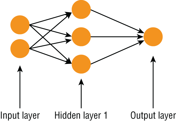
FIGURE 17.1 Structure of an artificial neural network (ANN)
ANNs are made up of units call neurons and are organized into a series of layers. There are three types of layers:
- Input layer: This is the layer that directly receives inputs for the computation. There is only one input layer in an artificial neural network.
- Output layer: This is the layer that provides the output of the computation. There can be one or more neurons in this layer, depending on the type of problem the network is used to solve.
- Hidden layer: This is a layer that sits between the input and the output layer. Neurons in the input layer are connected to neurons in the hidden layer, and neurons in the hidden layer are connected to neurons in the output layer. When each of the neurons in one layer is connected to every neuron in the previous layer, the network is called a fully connected network. A very simple neural network may not necessarily have a hidden layer, and complex neural networks such as deep-learning networks have several hidden layers, each with a large number of neurons in them.
Each of the connections between neurons has a weight value associated with it, and the weight multiplies the value of the neuron the connection originated from. Each neuron works by computing the sum of its inputs and passing the sum through a non-linear activation function. The output value of the neuron is the result of the activation function. Figure 17.2 depicts a very simple neural network with two neurons in the input layer and one neuron in the output layer.

FIGURE 17.2 A simple neural network
If x1, x2 are the values loaded into the neurons in the input layer, w1 , w2 are the connection weights between the input layer and the output layer, and f() is the activation function of the neuron in the output layer, then the output value of the neural network in Figure 17.2 is f(w1.x1 + w2.x2).
There are many different types of activation functions with their own advantages and disadvantages. The reason to have an activation function is to ensure that the network is not just a one big linear model. When a neural network is instantiated, the weights are set to random values. The process of training the neural network involves finding out the values of the weights.
The TensorFlow Python API is structured in a series of layers (Figure 17.3), with the topmost layer known as the Estimators API. Objects in the Estimators layer provide the ability to create entire neural networks with a single Python statement.
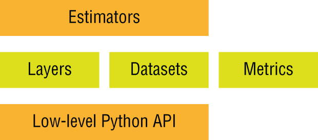
FIGURE 17.3 TensorFlow API architecture
The Estimators layer also provides a framework to train these networks. The intermediate layer consists of the Layers, Datasets, and Metrics APIs. The Layers API provides the ability to operate at the level of a neural network layer and create a complex neural network architecture by stitching together different types of layers. The lowest layer consists of low-level Python classes and functions that allow you to operate at the level of individual graph nodes such as tf.Variable, tf.placeholder, and tf.constant. In the next section you will create a simple linear regression model from scratch using the low-level Python API. In a subsequent section you will use the Estimators API to create a special kind of neural network called a Dense Neural Network (DNN) and use the network for a classification task. You can learn more about the TensorFlow APIs at https://www.tensorflow.org/guide.
Creating a Linear Regression Model with Google TensorFlow
In this section you will use an Amazon SageMaker notebook instance to train a linear regression model on the notebook instance with the low-level Python API provided by TensorFlow. The linear regression model will be trained on the Boston house prices toy dataset that is included in Scikit-learn. You can learn more about the Boston housing toy dataset at https://scikit-learn.org/stable/datasets/index.html#datasets. A copy of the dataset is included with the downloads that accompany this chapter. To better illustrate the process of using Google TensorFlow, the linear regression model will first be trained on a single feature of the dataset, and then modified to work with the remaining features.
To get started, log in to the AWS management console using the dedicated sign-in link for your development IAM user account. Navigate to the Amazon S3 management console and locate the awsml-sagemaker-source bucket (Figure 17.4).
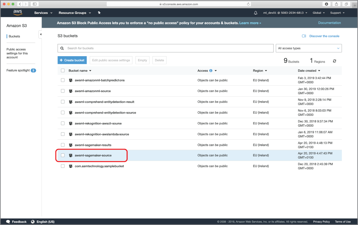
FIGURE 17.4 Accessing the Amazon S3 bucket that will contain the training and validation files
If you have not created the awsml-sagemaker-source bucket yet, refer to the section titled “Preparing Test and Training Data” in the previous chapter. Locate the datasets/boston_dataset folder in the resources that accompany this chapter and upload the boston_train.csv and boston_test.csv files to the Amazon S3 bucket (Figure 17.5).
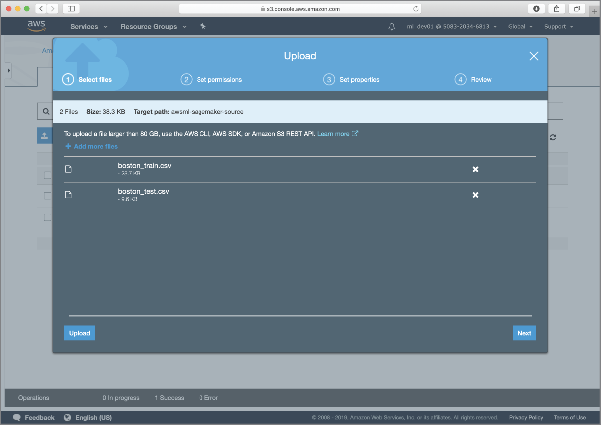
FIGURE 17.5 Uploading the pre-split training and test data files to the Amazon S3 bucket
Techniques to prepare training and test datasets were covered in Chapter 5. A Jupyter Notebook file called PreparingTheBostonDataset.ipynb is included with the resources that accompany this chapter. This file contains the Python code that was used to generate the boston_train.csv and boston_test.csv files on an instance of Jupyter Notebook running locally on the author's computer.
After you have uploaded the files to Amazon S3, use the Services drop-down menu to switch to the Amazon SageMaker management console and create a new ml.t2-medium notebook instance called tensorflow-models. Amazon SageMaker will, by default, select the same IAM role that was created for you when you created the kmeans-iris-flowers notebook instance in the previous chapter.
- NOTE If you did not create the notebook instance in the previous chapter, you will need to create a new IAM role that will be assumed by the notebook instance. Refer to the section titled “Creating an Amazon SageMaker Notebook Instance” in the previous chapter for instructions on creating this IAM role.
When the tensorflow-models notebook instance is ready, you will see it listed in your Amazon SageMaker management console with the status of “In Service” (Figure 17.6).
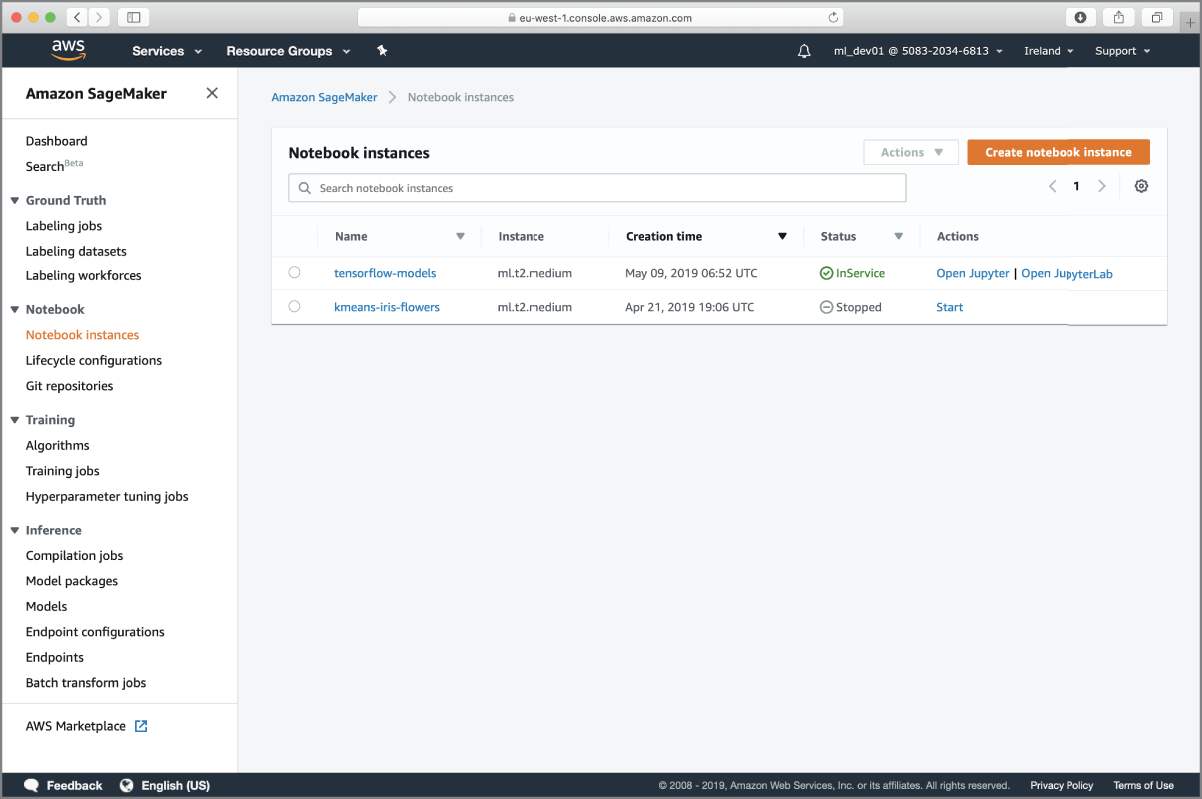
FIGURE 17.6 Amazon SageMaker management console showing the new notebook instance
Click the Open Jupyter link to access the Jupyter Notebook server running on your tensorflow-models notebook instance and create a new notebook file called TF_SingleFeatureRegression_SGD using the conda_tensorflow_p36 kernel. Execute the following code snippet in an empty notebook cell to load the boston_train.csv and boston_test.csv files from Amazon S3 into Pandas dataframes, and separate the feature variables and target into separate dataframes:
import boto3import sagemakerimport ioimport pandas as pdimport numpy as np# load training and validation dataset from Amazon S3s3_client = boto3.client('s3')s3_bucket_name='awsml-sagemaker-source'response = s3_client.get_object(Bucket='awsml-sagemaker-source', Key='boston_train.csv')response_body = response["Body"].read()df_boston_train = pd.read_csv(io.BytesIO(response_body), header=0, delimiter=",", low_memory=False)response = s3_client.get_object(Bucket='awsml-sagemaker-source', Key='boston_test.csv')response_body = response["Body"].read()df_boston_test = pd.read_csv(io.BytesIO(response_body), header=0, index_col=False, delimiter=",", low_memory=False)# extract features and target variable into separate datasets.df_boston_train_target = df_boston_train.loc[:,['price']]df_boston_train_features = df_boston_train.drop(['price'], axis=1)df_boston_test_target = df_boston_test.loc[:,['price']]df_boston_test_features = df_boston_test.drop(['price'], axis=1)
The df_boston_train dataset has 14 columns. The first column is called price and is the target variable, and the remaining 13 columns are the feature variables. The description of the 13 feature variables is present at https://scikit-learn.org/stable/datasets/index.html#datasets. You can inspect the first five rows of the df_boston_train dataframe by using the dataframe's head() method (Figure 17.7).
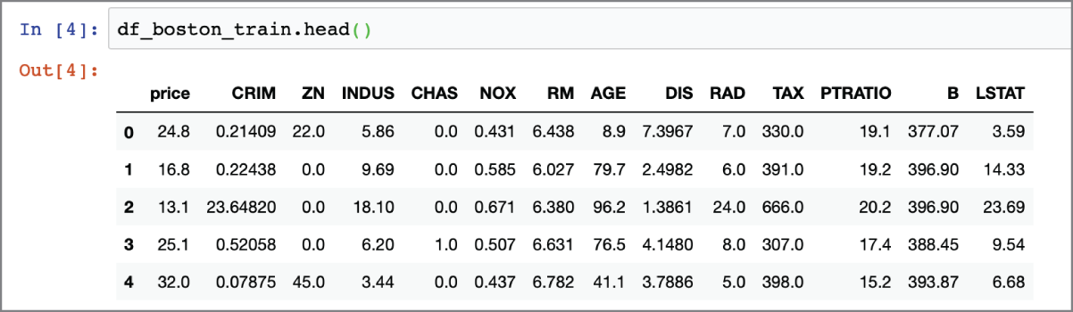
FIGURE 17.7 Inspecting the first five rows of the Boston housing dataset
Let's now build a linear regression model using the low-level TensorFlow Python API that attempts to predict the value of the price target attribute from a single feature variable. The complete code that you can execute in a notebook cell will be presented at the end of this section; for now, let's explore the process of building and training a model with the low-level TensorFlow API.
You can choose any feature variable. The code in this section assumes you are using the first feature of the dataset, which is called CRIM and represents the per-capita crime rate. Recall from Chapter 4 that a linear regression model attempts to fit a straight line (or hyperplane) to the set of points that make the training data and uses the line to make predictions on future values. The general equation of a linear regression model for N features is:
Where:
- w1, w2, … wn are the coefficients associated with the features X1, X2, … Xn respectively.
- Y is the predicted value (target value).
- Xi's are the input features.
- c is a constant term, also known as the bias term or intercept.
Since we are trying to build a model from a single feature, this equation reduces to:
The aim of model training will be to find the value of w1 and c that will result in the best possible predictions. The quality of predictions will be measured using the mean squared error (MSE) metric, which is illustrated in Figure 17.8.
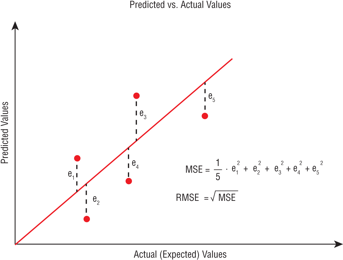
FIGURE 17.8 Mean squared error metric
The process of building a model with TensorFlow involves defining a tree-like structure called a computation graph, and the process of training the model is achieved by evaluating the root node of the computation graph in a session and feeding the graph with the training data. Let's now define the computation graph.
Since we are building a linear regression model that takes one input feature and predicts the value of one target variable, we will need to provide two inputs to the TensorFlow graph during model training. The first will be an array of values called x1, which will contain the values in the CRIM column of the df_boston_train_features dataset. The second input to the model training process will be an array of values called y_actual that will contain the values of the price column from the df_boston_train_target dataset. Values of the price column are what we want the model to predict, but during the model-training process we will provide both the CRIM and price values and compute the optimum values of w1 and c.
Values that you need provide as inputs to a computation graph at runtime are represented using placeholder nodes. You create placeholder nodes using the tf.placeholder() function. The following snippet creates two placeholder nodes called x1 and y_actual and adds the nodes to the default computation graph:
import tensorflow as tftf.reset_default_graph()x1 = tf.placeholder(tf.float32, [None, 1], name="x1")y_actual = tf.placeholder(tf.float32, [None, 1], name="y_actual")
- NOTE The standard alias for TensorFlow in Python projects is
tf. TensorFlow is typically imported into a Python project using the following statement:import tensorflow as tfThe standard behavior of TensorFlow is to add any nodes you create to the default computation graph. It is possible to create additional graph objects and attach nodes to these other graphs.
The
tf.reset_default_graph()statement is used to delete any nodes from the default computation graph.
TensorFlow will expect you to feed values for all placeholder nodes when you execute the computation graph in a session, and we will see how to do that shortly. All data that flows through a computation graph is represented as n-dimensional matrices called tensors, and therefore a placeholder is a tensor. The dimensions of the x1 and y_actual tensors have been specified as [None, 1], which means both x1 and y_actual are tensors that have any number of rows, and a single column. The data type of the tensor elements is defined as float32, which is a 32-bit floating-point number. You can learn more about the tf.placeholder() function at https://www.tensorflow.org/api_docs/python/tf/placeholder. Figure 17.9 depicts the structure of the computation graph after the two placeholder nodes are created.
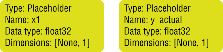
FIGURE 17.9 Computation graph with two placeholder nodes
Your linear regression model will also contain two variables: the weight w1 corresponding to the one input feature and the intercept term c. The objective of model training will be to use the computation graph to find the values of w1 and c. Quantities whose values can be changed as a result of executing the graph are known as variables in TensorFlow, and are represented as instances of the tf.Variable class. Typically, you will create tf.Variable instances for all quantities that you wish to compute. Just like placeholders, variables are also tensors. However, unlike placeholders, you do not feed the value of variables into the computation graph at runtime; instead, they are assigned an initial value and then the value of the variable is updated as different nodes of the graph are evaluated. You can create variables using the tf.Variable() constructor or the tf.get_variable() function. The following statements define two variables, w1 and c, using the tf.Variable() constructor:
w1 = tf.Variable(tf.zeros([1,1]), name="w1")c = tf.Variable(tf.zeros([1]), name="c")
When you create a variable, you need to provide a default value; the shape of the variable tensor is inferred from the shape of the default value. The preceding statements make use of the tf.zeros() function to create tensors that are used as default values for the w1 and c variables. The tf.zeros() function creates tensors that have all elements set to 0. You can learn more about the tf.zeros() function at https://www.tensorflow.org/api_docs/python/tf/zeros. Even though you have specified the initial value of the variable as a constructor argument, the values are not assigned to those variables until the graph is executed in a session. Figure 17.10 depicts the structure of the computation graph after the two variable nodes are created.
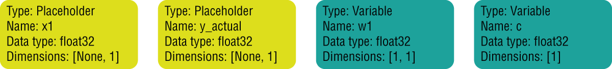
FIGURE 17.10 Computation graph with two variable nodes
Now that you have created placeholder nodes and variable nodes in the computation graph, you can use the tf.matmul() operator to create an operation node that will contain the matrix product of the tensors in the w1 and x1 nodes. You can learn more about the tf.matmul() operator at https://www.tensorflow.org/api_docs/python/tf/linalg/matmul. The following statement adds a new node called temp to the computation graph, the value of which will be the tensor obtained by multiplying the tensors w1 and x1:
temp = tf.matmul(x1,w1)Figure 17.11 depicts the structure of the computation graph after the matrix multiplication node has been added.
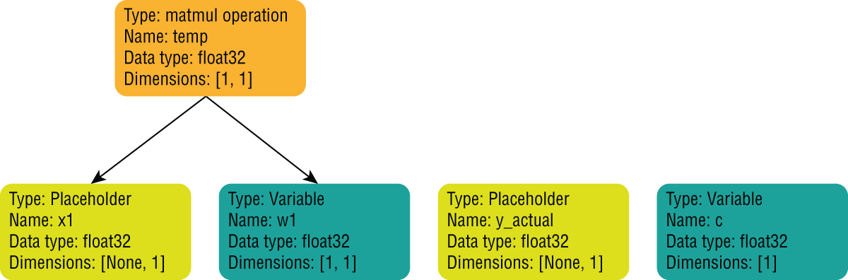
FIGURE 17.11 Computation graph after the multiplication of w1 and x1 nodes
Let's now create a new operation node in the computation graph, the value of which is the sum of the temp tensor and the tensor in variable c. We can do this by using the + arithmetic operator as follows:
y_predicted = temp + cFigure 17.12 depicts the structure of the computation graph after the y_predicted node has been added.
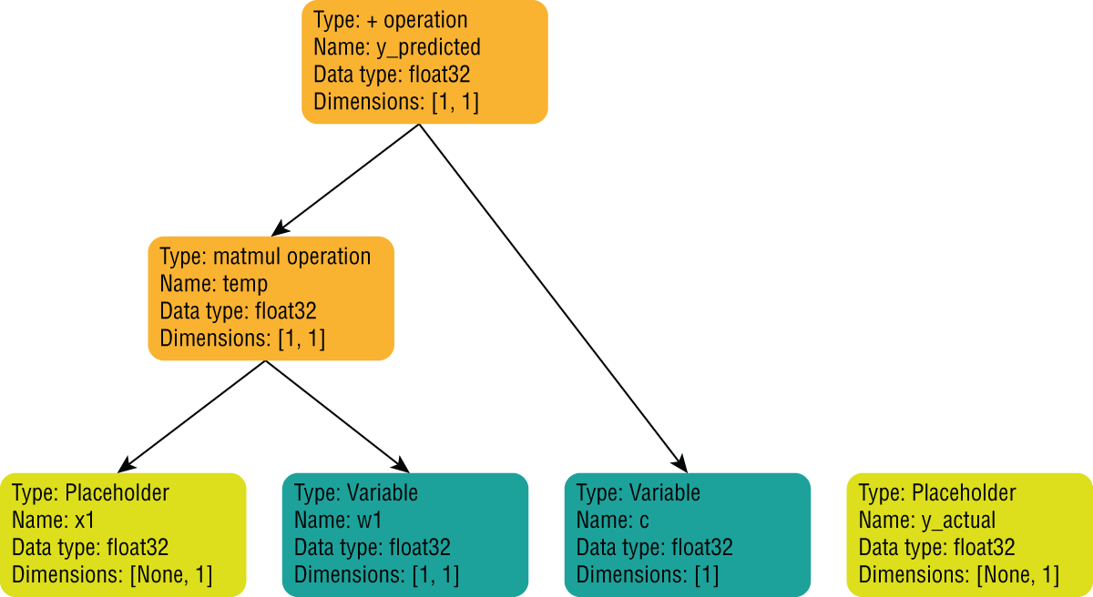
FIGURE 17.12 Computation graph with y_predicted
The y_predicted node represents your linear regression model. However, since the default values of w1 and c are tensors with zeros in them, the y_predicted values will all be zero, regardless of the values you feed into the x1 placeholder.
What you need to do is work out the best values for the w1 and c tensors, and in order to do so, you will need to feed the expected values of the target variable price into the y_actual placeholder, compute the value of a cost function that captures the error in prediction between the actual and predicted values, and adjust the values of w1 and c so as to minimize the value of the cost function.
Let's now add nodes to the computation graph to compute the value of a cost function. There are many kinds of cost functions, such as MSE, RMSE, MAE, etc., and the low-level TensorFlow API provides the ability to create operation nodes that can be combined together to compute the value of common cost functions. In this section you will use the mean squared error (MSE) cost function, and the cost function can be computed in three steps:
- Use the
–arithmetic operator to create an operation node in the graph to compute the difference between the actual and predicted values. - Use the
tf.square()operator to create another operation node that can square the difference computed in the previous step. - Use the
tf.reduce:mean()function to create a third operation node that can compute the mean of the values computed in the previous step.
The following code snippet adds nodes to the computation graph to perform these three steps:
# compute cost function# MSE between predicted and actual valuesdiff = y_predicted – y_actualsquare_diff = tf.square(diff)mse_cost = tf.reduce:mean(square_diff)
The tf.reduce:mean() operator provided by TensorFlow is equivalent to the NumPy mean() function, and you can learn more about the tf.reduce:mean() operator at https://www.tensorflow.org/api_docs/python/tf/math/reduce:mean. Figure 17.13 depicts the structure of the computation graph after the nodes to compute the MSE cost have been added.
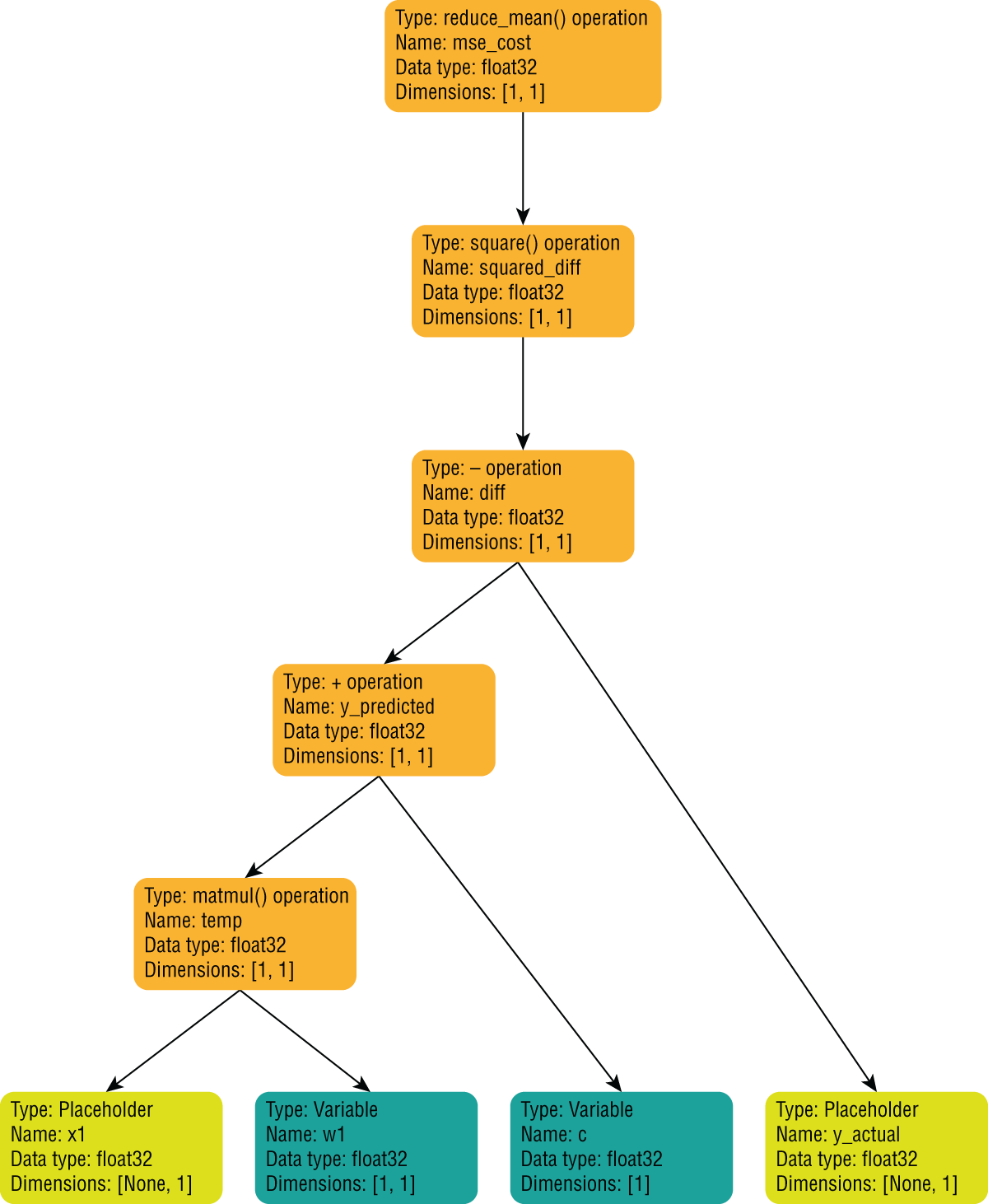
FIGURE 17.13 Computation graph that contains nodes to compute the MSE cost function
Now that you have a node in your graph that represents the cost function, you need to tweak the values of the variables w1 and c so as to reduce the value of the cost function. One solution is to try every possible combination of w1 and c and pick the one that results in the lowest value of the cost function. This approach will return the best possible values of w1 and c but can be impractical to compute because of the sheer number of possibilities. If searching for the best possible values is not practical, you will need to search for good-enough values, and in order to do so you will need to apply an optimization strategy to reduce the size of the search space. Various optimization algorithms are used by data scientists and the one you are going to use in this section is called gradient descent (GD) optimization.
An in-depth discussion of gradient descent optimization is outside the scope of this book. You can learn more about the gradient descent technique at https://developers.google.com/machine-learning/crash-course/reducing-loss/gradient-descent. Gradient descent is a popular optimization algorithm and is based on an assumption that the three-dimensional plot of the values of the cost function mse_cost, w1, and c is bowl shaped (concave), and it has a single minimum value. With this assumption, the gradient descent algorithm computes the value of the derivate (gradient) of the point [mse_cost, w1, c] and uses the sign of the derivative to work out the direction in which the value of the cost function should be moved. A positive value would indicate that the optimal point on the surface of the bowl-shaped curve is higher up (toward the rim of the bowl), and a negative value would indicate that the optimal point is somewhere lower down toward the trough. A new point is then selected on the bowl-shaped curve by moving a small amount in the direction indicated by the gradient and the corresponding w1 and c values are selected. This process then repeats iteratively for a fixed number of iterations, and the best value arrived at during the iterations is selected.
Fortunately, you do not need to implement the gradient descent algorithm from scratch in TensorFlow, and instead can create an instance of the tf.GradientDescentOptimizer class to get an optimizer object, and then use the minimize() method of the optimizer object to get an operation node that can both compute the gradient and use the gradient to tweak the values of the variables that impact the value of the cost function. The following snippet demonstrates the use of the tf.GradientDescentOptimizer class to add an operation node to the computation graph. You can learn more about this class at https://www.tensorflow.org/api_docs/python/tf/train/GradientDescentOptimizer.
# create a root node - a gradient descent optimizer, setup to optimize the# mse_costlearning_rate = 0.000001train_step = tf.train.GradientDescentOptimizer(learning_rate).minimize(mse_cost)
Figure 17.14 depicts the structure of the computation graph after the optimizer operation has been added.
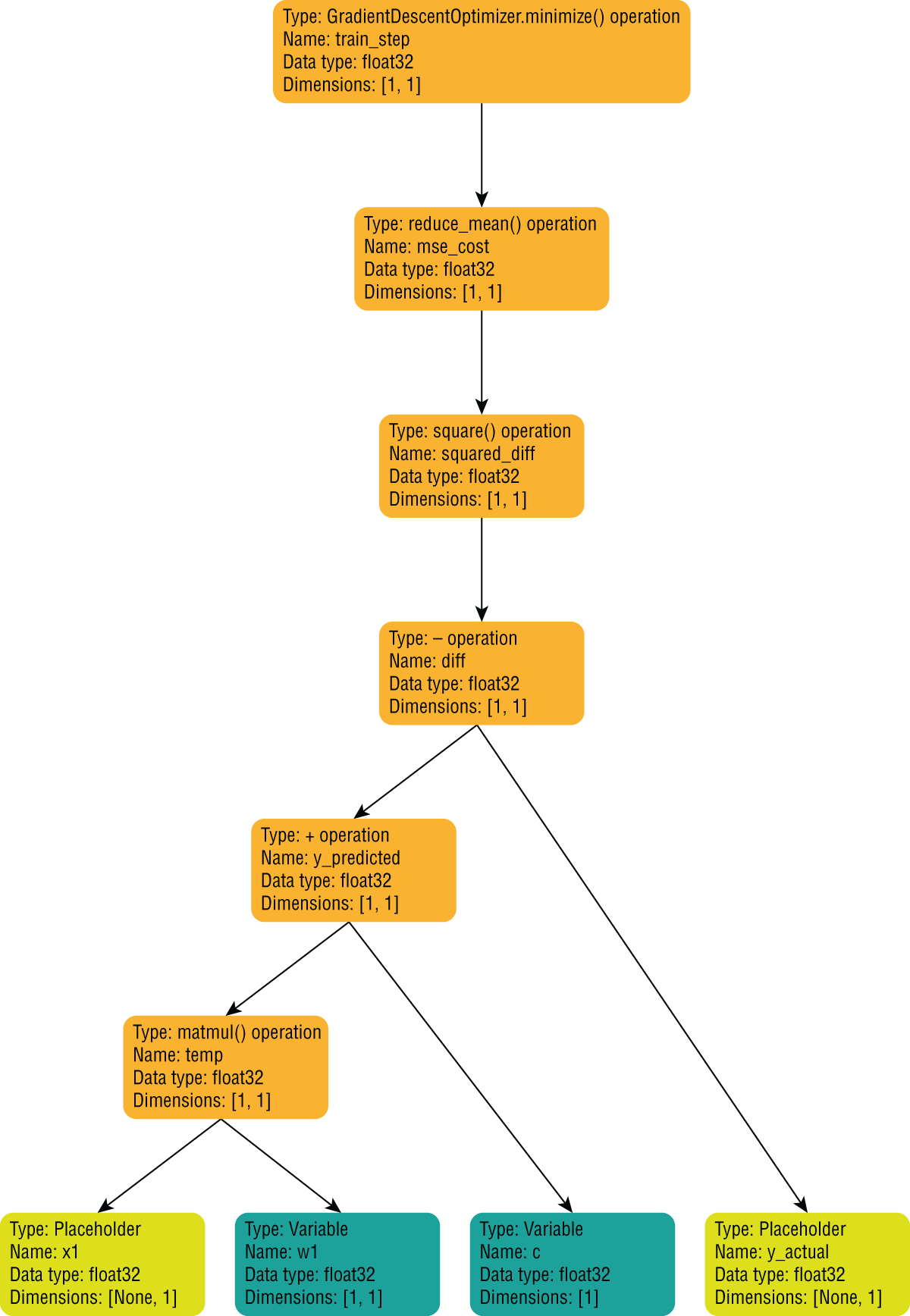
FIGURE 17.14 Computation graph that contains the operation to optimize the cost function
Now that you have created the computation graph, you need to run the graph in a session, which involves creating a tf.Session object, initializing the variables of the graph, feeding values into the placeholders, and evaluating the values of one or more nodes of the graph.
The following snippet prepares two arrays, xin and yin, that contain the values you will feed into the placeholder nodes once you run the computation graph in a session:
# extract CRIM feature and target variable into arrays so that# these can be fed into the computation graph via the placeholders# created earlier.xin = df_boston_train_features['CRIM'].valuesyin = df_boston_train_target['price'].values
It is important to note that you do not have to start evaluating the graph at the root node and can choose to evaluate the value of any node in the graph. TensorFlow will evaluate the values of any child nodes needed to compute the value of the node you want to evaluate. Instead of initializing every variable in your computation graph one by one, you can use the tf.global_variables_initializer() function to add an initializer node to the computation graph. This node when executed within a session will initialize all the variables in the computation graph with default values. The following snippet creates a tf.Session object, and initializes the values of all the variables in the default computation graph using the tf.global_variables_initializer() function:
with tf.Session() as sess:# use a global_variable_initializer node to initialize# variables all variables in the graph (w1 and c)init_node = tf.global_variables_initializer()sess.run(init_node)
The call to the tf.global_variables_initializer() function adds an initializer node to the graph, but the actual variable initialization happens when the next line, sess.run(init_node), is executed. The run() method of the tf.Session object can be used to execute any node of the computation graph. You can learn more about tf.Session at https://www.tensorflow.org/api_docs/python/tf/Session.
- NOTE The reason to use the
with-asstatement is to ensure that you do not explicitly need to close the session object once you have finished using it.If you did not want to use the
with-asstatement, the equivalent lines of code would have been:sess = tf.Session()init_node = tf.global_variables_initializer()sess.run(init_node)sess.close()Forgetting to call
sess.close()will result in the resources associated with the session not being freed, and in order to avoid the problem altogether, Python programmers use thewith-asstatement when creating sessions.
With the variables initialized, the following code snippet will feed each item of the xin and yin Python arrays into the x1 and y_actual placeholder nodes one element at a time, and it will evaluate the train_step node of the graph. The values of the w1 and c graph variables that result in the lowest value of the cost function will be stored in the best_w1, best_c, and lowest_cost Python variables. These statements must be executed within the scope of the with-as statement:
# for each observation, evaluate the node called train_step# which will in turn update w1 and c so as to minimize# the cost function.num_elements = df_boston_train_features.shape[0]best_w1 = 0.0best_c = 0.0lowest_cost = 100000.00for i in range(num_elements):input_dict={x1:[[xin[i]]], y_actual:[[yin[i]]]}sess.run(train_step, feed_dict=input_dict)computed_w1 = sess.run(w1)computed_c = sess.run(c)computed_cost = sess.run(mse_cost, feed_dict=input_dict)if computed_cost < lowest_cost:lowest_cost = computed_costbest_w1 = computed_w1best_c = computed_cprint ("End of iteration %d, w1=%f, c=%f, cost=%f" % (i, computed_w1, computed_c, computed_cost))print ("End of training, w1=%f, c=%f, lowest_cost=%f" % (best_w1, best_c, lowest_cost))
In this snippet, a Python for loop is used to enumerate the contents of the xin and yin array and feed each element into placeholder nodes x1 and y_actual, one element at a time. TensorFlow requires that the values of any relevant placeholder nodes are fed into the computation graph using a dictionary object in the call to the sess.run() function. To understand how the model is trained, assume that for the first iteration i = 1, xin[i] = 10 and yin[i] = 20. Substituting these values, the call to sess.run() becomes
sess.run(train_step, feed_dict={x1:[[10]], y_actual:[[20]]})The node being evaluated in the call to sess.run() is the train_step node is defined as:
train_step = tf.train.GradientDescentOptimizer(learning_rate).minimize(mse_cost)In order to evaluate the train_step node, TensorFlow will need to access the tensor in the mse_cost node, and as a result, will need to evaluate the mse_cost node of the graph. The mse_cost node is defined as:
mse_cost = tf.reduce:mean(square_diff)TensorFlow will now evaluate the value of the square_diff node, which is defined as:
square_diff = tf.square(diff)This recursive evaluation process will continue until TensorFlow needs to evaluate the xin and yin placeholder nodes. When that happens, TensorFlow will use the values 10 and 20 provided in the feed_dict parameter to sess.run() for these placeholder nodes. The initial values of the w1 and c variable nodes will be 0, and the mse_cost tensor will be computed using these values. When the GradientDescentOptimizer node is evaluated, it will adjust the values of the w1 and c variable nodes to reduce the value of mse_cost by a small amount. Since the global_variables_initializer node is not executed in the for loop, the variables will retain their values across iterations of the loop.
Once the train_step node has been evaluated, the tensors in the w1 and c graph nodes will contain the optimized model parameters. To read these values, you will need to evaluate the w1 and c nodes in separate sess.run() statements:
computed_w1 = sess.run(w1)computed_c = sess.run(c)
Even though TensorFlow has computed the value of the w1 and c nodes while evaluating the train_step node, the subsequent calls to sess.run(w1) and sess.run(c) will result in TensorFlow evaluating the computation graph again. Since these variable nodes do not have any dependent nodes, there will be no recursion involved, and TensorFlow will return the value of the tensors stored in these variable nodes.
Astute readers may have noticed that by feeding xin and yin values one element at a time, the gradient descent optimization process is trying to optimize the cost function for each element independently, and not trying to optimize for a better overall prediction across all the values of xin and yin. When gradient descent optimization is used in this manner, for one data point at a time, it is known as stochastic gradient descent.
All of the model building, training, and optimization steps discussed so far in this section are presented together in the following snippet. The complete code is also available in the TF_SingleFeatureRegression_SGD notebook file included with this chapter's resources:
# train a linear regression model on a single feature# the general equation for linear regression is:# y = w1x1 + w2x2 + … wnxn + c## in case of a single feature, the equation reduces to:# y = w1x1 + cimport tensorflow as tftf.reset_default_graph()## define a TensorFlow graph## what you will provide:# x1 = one-dimensional column array of features# y_actual = one-dimensional column array of expected values/labelsx1 = tf.placeholder(tf.float32, [None, 1], name="x1")y_actual = tf.placeholder(tf.float32, [None, 1], name="y_actual")# what you are interested in:# w1, c weight and bias term (intercept)w1 = tf.Variable(tf.zeros([1,1]), name="w1")c = tf.Variable(tf.zeros([1]), name="c")# compute y_predicted = w1x1 + ctemp = tf.matmul(x1,w1)y_predicted = temp + c# compute cost function# MSE between predicted and actual valuesdiff = y_predicted - y_actualsquare_diff = tf.square(diff)mse_cost = tf.reduce:mean(square_diff)# create a root node - a gradient descent optimizer, setup to optimize the# mse_cost function.learning_rate = 0.000001train_step = tf.train.GradientDescentOptimizer(learning_rate).minimize(mse_cost)# extract CRIM feature and target variable into arrays so that# these can be fed into the computation graph via the placeholders# created earlier.xin = df_boston_train_features['CRIM'].valuesyin = df_boston_train_target['price'].values## execute the graph#with tf.Session() as sess:# use a global_variable_initializer node to initialize# variables all variables in the graph (w1 and c)init_node = tf.global_variables_initializer()sess.run(init_node)# for each observation, evaluate the node called train_step# which will in turn update w1 and c so as to minimize# the cost function.num_elements = df_boston_train_features.shape[0]best_w1 = 0.0best_c = 0.0lowest_cost = 100000.00for i in range(num_elements):input_dict={x1:[[xin[i]]], y_actual:[[yin[i]]]}sess.run(train_step, feed_dict=input_dict)computed_w1 = sess.run(w1)computed_c = sess.run(c)computed_cost = sess.run(mse_cost, feed_dict=input_dict)if computed_cost < lowest_cost:lowest_cost = computed_costbest_w1 = computed_w1best_c = computed_cprint ("End of iteration %d, w1=%f, c=%f, cost=%f" % (i, computed_w1, computed_c, computed_cost))print ("End of training, w1=%f, c=%f, lowest_cost=%f" % (best_w1, best_c, lowest_cost))
If you execute this code in an empty notebook cell, you will see log messages below the notebook cell, listing the values of w1, c, and the cost function at each iteration. A section of the log messages corresponding to the last few iterations is presented here:
As you can see, the cost function is fluctuating randomly with each iteration—sometimes it goes up, and sometimes it goes down. This is because we are feeding the dataset one point at a time.
At the end of the training, the values of best_w1 and best_c1 represent the parameters of the trained model and can be used to make predictions on the test set using the linear regression equation Y = w1X1 + c. This is demonstrated in the following snippet:
# use best_w1 and best_c to make predictions on all observations in the test setpredictions = df_boston_test_features['CRIM'].values * best_w1 + best_c
Once you have the predictions, you can use Scikit-learn to compute the MSE across all the predictions over the test set using the values of best_w1 = 0.016363 and best_c = 0.005673 as follows:
# compute MSE on test setfrom sklearn.metrics import mean_squared_errormse_test = mean_squared_error(np.transpose(df_boston_test_target.values), predictions)
The value of the mean squared error can be examined using the Python print statement, and comes out as a rather high value—which indicates that the model is performing quite poorly:
This poor performance is to be expected for a number of reasons, the top two of which are that we are using just one feature of the dataset, and our optimization step is not trying to reduce the value of the cost function over the entire dataset. This code can easily be modified to work with multiple features of the dataset and perform batch gradient descent. The modified version of this code is provided in the TF_MultiFeatureRegression_BatchGradientDescent notebook file as part of the resources that accompany this chapter. The model training and optimization code is presented here, with the key differences highlighted in boldface:
# train a linear regression model on a single feature# the general equation for linear regression is:# y = w1x1 + w2x2 + … wnxn + c## in case of a single feature, the equation reduces to:# y = w1x1 + cimport tensorflow as tftf.reset_default_graph()## define a TensorFlow graph## what you will provide:# x1 = one-dimensional column array of features# y_actual = one-dimensional column array of expected values/labelsx1 = tf.placeholder(tf.float32, [None, 1], name="x1")y_actual = tf.placeholder(tf.float32, [None, 1], name="y_actual")# what you are interested in:# w1, c weight and bias term (intercept)w1 = tf.Variable(tf.zeros([1,1]), name="w1")c = tf.Variable(tf.zeros([1]), name="c")# compute y_predicted = w1x1 + cy_predicted = tf.matmul(x1,w1) + c# compute cost function# MSE between predicted and actual valuesmse_cost = tf.reduce:mean(tf.square(y_predicted - y_actual))# create a root node - a gradient descent optimizer, setup to optimize the# mse_cost function.learning_rate = 0.00001train_step = tf.train.GradientDescentOptimizer(learning_rate).minimize(mse_cost)## execute the graph#with tf.Session() as sess:# use a global_variable_initializer node to initialize# variables all variables in the graph (w1 and c)init = tf.global_variables_initializer()sess.run(init)# extract CRIM feature and target variable into arraysxin = df_boston_train_features['CRIM'].valuesyin = df_boston_train_target['price'].valuesxin = np.transpose([xin])yin = np.transpose([yin])# for each observation, evaluate the node called train_step# which will in turn update w1 and c so as to minimize# the cost function.best_w1 = 0.0best_c = 0.0lowest_cost = 100000.00num_epochs = 100000for i in range(num_epochs):input_dict={x1:xin, y_actual:yin}sess.run(train_step, feed_dict=input_dict)computed_w1 = sess.run(w1)computed_c = sess.run(c)computed_cost = sess.run(mse_cost, feed_dict=input_dict)if computed_cost < lowest_cost:lowest_cost = computed_costbest_w1 = computed_w1best_c = computed_cprint ("End of epoch %d, w1=%f, c=%f, cost=%f" % (i, computed_w1, computed_c, computed_cost))print ("End of training, best_w1=%f, best_c=%f, lowest_cost=%f" % (best_w1, best_c, lowest_cost))
As you can see, the entire contents of xin and yin are fed into the computation graph, and not just once, but 100,000 times. Presenting the entire training set multiple times ensures that the gradient descent optimizer is able to find better values of w1 and c. The number of times the training set is presented during model optimization is called the number of training epochs, and this value is hardcoded to 100000 in the preceding snippet. In effect, the learning_rate and num_epochs Python variables are hyperparameters of the linear regression model.
If you execute this code in an empty notebook cell, you will see log messages below the notebook cell, listing the values of w1, c, and the cost function at the end of each training epoch. A selection of the log messages corresponding to different training epochs is presented here:
As you can see, the cost function is not randomly fluctuating with each epoch anymore, but instead is steadily decreasing, which is more in line with what you would expect from an optimization process.
At the end of the training, the values of best_w1=-0.222625 and best_c1=19.488808 represent the parameters of the trained model and can be used to make predictions on the test set using the linear regression equation Y = w1X1 + c. This is demonstrated in the following snippet:
# use best_w1 and best_c to make predictions on all observations in the test setpredictions = df_boston_test_features['CRIM'].values * best_w1 + best_c
Once you have the predictions, you can use Scikit-learn to compute the MSE across all the predictions over the test set using the values of best_w1=-0.222625 and best_c1=19.488808 as follows:
# compute MSE on test setfrom sklearn.metrics import mean_squared_errormse_test = mean_squared_error(np.transpose(df_boston_test_target.values), predictions)
The value of the mean squared error can be examined using the Python print statement, and comes out to be a significantly lower value—which indicates that the model is performing significantly better:
Training and Deploying a DNN Classifier Using the TensorFlow Estimators API and Amazon SageMaker
In the previous section, you learned to create a linear regression model from scratch using the low-level TensorFlow Python API. In this section you will use the high-level TensorFlow Estimators API to train a Dense Neural Network (DNN)–based classifier on the popular Iris flowers dataset.
You will write your TensorFlow code in a Python script file and upload it to your Amazon SageMaker notebook instance. You will then use the AWS SageMaker SDK for Python from a Jupyter Notebook running on your notebook instance to create a training job. The training job will create a dedicated training instance on the AWS cloud and deploy your TensorFlow model-training code onto the instance. When the training completes, your trained model will be stored in an Amazon S3 bucket, after which you will use another function provided by the AWS SageMaker Python SDK to deploy the trained model to a dedicated prediction instance and create an HTTPS prediction endpoint. Finally, you will use the AWS SageMaker SDK for Python to interact with this prediction endpoint from your Jupyter Notebook file to make predictions on data the model has not seen.
A dedicated training instance is an EC2 instance that is used to train a model from data in an Amazon S3 bucket and save the trained model to another Amazon S3 bucket. However, unlike a notebook instance, a dedicated training instance does not have a Jupyter Notebook server and is terminated automatically once the training process is complete. Dedicated training instances are created from Docker images. Amazon SageMaker provides Docker images for training and deploying models that have been created using the TensorFlow Estimators API. The Docker image used for training includes TensorFlow, Python, and a number of other libraries such as NumPy and Pandas. The Docker image used to deploy trained models includes TensorFlow Serving, which is a server product from Google that allows TensorFlow models to be deployed in production environment and accessed via REST APIs. Amazon's Docker images are stored in Docker registries within each AWS region. You can find the paths to the Docker registries for TensorFlow Docker images in each supported region at https://docs.aws.amazon.com/sagemaker/latest/dg/pre-built-docker-containers-frameworks.html.
The dedicated EC2 training instances, once created, will need to assume an IAM role that will allow code running in the training instances access to other resources in your AWS account, such as Amazon S3 buckets that contain the training data. Since the IAM role that is used to create your notebook instance has the correct permissions to access the relevant AWS resources, the most common approach is to use the same IAM role for the EC2 training instances.
To get started, launch the tensorflow-models notebook instance and use the Upload button to upload the TF_DNN_iris_training_script.py file provided with the resources that accompany this chapter (Figure 17.15).
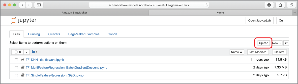
FIGURE 17.15 Uploading a file to a notebook instance
The Python code within this file is presented here:
import argparseimport numpy as npimport pandas as pdimport osimport tensorflow as tfdef estimator_fn(run_config, params):feature_columns = [tf.feature_column.numeric_column(key='sepal_length'),tf.feature_column.numeric_column(key='sepal_width'),tf.feature_column.numeric_column(key='petal_length'),tf.feature_column.numeric_column(key='petal_width')]return tf.estimator.DNNClassifier(feature_columns=feature_columns,hidden_units=[10, 10],n_classes=3,config=run_config)def train_input_fn(training_dir, params):# read input file iris_train.csv .input_file = os.path.join(training_dir, 'iris_train.csv')df_iris_train = pd.read_csv(input_file, header=0, engine="python")# convert categorical target attribute 'species' from strings to integersdf_iris_train['species'] = df_iris_train['species'].map({'Iris-setosa':0,'Iris-virginica':1,'Iris-versicolor':2})# extract numpy data from a DataFramelabels = df_iris_train['species'].valuesfeatures = {'sepal_length': df_iris_train['sepal_length'].values,'sepal_width': df_iris_train['sepal_width'].values,'petal_length': df_iris_train['petal_length'].values,'petal_width': df_iris_train['petal_width'].values}return features, labelsdef eval_input_fn(training_dir, params):# read input file iris_test.csv .input_file = os.path.join(training_dir, 'iris_test.csv')df_iris_test = pd.read_csv(input_file, header=0, engine="python")# convert categorical target attribute 'species' from strings to integersdf_iris_test['species'] = df_iris_test['species'].map({'Iris-setosa':0,'Iris-virginica':1,'Iris-versicolor':2})# extract numpy data from a DataFramelabels = df_iris_test['species'].valuesfeatures = {'sepal_length': df_iris_test['sepal_length'].values,'sepal_width': df_iris_test['sepal_width'].values,'petal_length': df_iris_test['petal_length'].values,'petal_width': df_iris_test['petal_width'].values}return features, labelsdef serving_input_fn(params):feature_spec = {'sepal_length': tf.FixedLenFeature(dtype=tf.float32, shape=[1]),'sepal_width': tf.FixedLenFeature(dtype=tf.float32, shape=[1]),'petal_length': tf.FixedLenFeature(dtype=tf.float32, shape=[1]),'petal_width': tf.FixedLenFeature(dtype=tf.float32, shape=[1])}returntf.estimator.export.build_parsing_serving_input_receiver_fn(feature_spec)()
The high-level TensorFlow Estimators API is contained in the tf.estimators package. You can create a model using one of the pre-made Estimators contained in this package or create your own custom Estimator. As of when this chapter was written, Amazon SageMaker only allows you to build and deploy models that are built using the Estimators API onto prediction instances. If you use the low-level TensorFlow Python API, you can train your model on a notebook instance but cannot deploy it onto the Amazon cloud and create an HTTPS prediction endpoint. It is possible to create a custom Estimator object and use this to wrap your low-level model-building code, but this is an advanced topic and beyond the scope of this book. If you want to learn more about building custom Estimators, refer to https://www.tensorflow.org/guide/custom_estimators.
The model that you will be training in this section will use a pre-made Estimator called tf.estimators.DNNClassifier. The advantage of using pre-made Estimators is that you do not need to build a computation graph or manage a session. You can use a pre-made Estimator with minimal effort, out of the box, without necessarily understanding how it works. Since all Estimator objects implement a common interface, it is possible to switch to different model architectures with minimal effort. The neural network classifier will consist of an input layer with 4 neurons, 2 hidden layers with 10 neurons each, and an output layer with 3 neurons. All neurons in a layer are fully connected with the neurons in the previous layer. The architecture of the neural network is depicted in Figure 17.16.
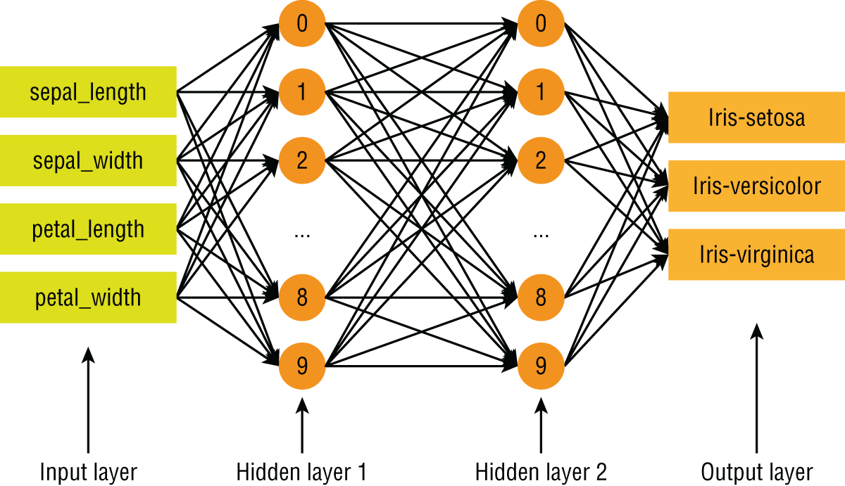
FIGURE 17.16 Architecture of neural-network–based classification model
The four input neurons correspond to the four features of the Iris dataset, and each of these neurons accepts continuous numeric floating-point input values. The three output neurons correspond to the three target classes, and the values of these will also be a continuous numeric floating-point value, which will represent the class-wise prediction probability.
Let's briefly examine the training script file TF_DNN_iris_training_script.py. Amazon SageMaker requires that a script file to train a TensorFlow model implements the following functions:
- Any one of these three functions:
-
estimator_fn: This function is used when you are building a model using a pre-built TensorFlow Estimator. The function is expected to return an instance of a pre-built TensorFlowEstimatorobject that will train the model. -
keras_model_fn: This function is used when you are building a model using the Keras library. -
model_fn: This function is used when you are building a model from scratch. The function is expected to return anEstimatorSpecobject, which will be used to generate anEstimatorobject.
-
-
train_input_fn: This function is responsible for reading training data from your data sources, preprocessing the data, and converting the data into a format that the Estimator can use. -
eval_input_fn: This function is responsible for reading evaluation data from your data sources, preprocessing the data, and converting the data into a format that the Estimator can use. -
serving_input_fn: This function is responsible for preprocessing the data that you submitted with your prediction requests and preparing them for the model.
Since you are creating a model using a pre-built Estimator, your script implements estimator_fn as follows:
def estimator_fn(run_config, params):feature_columns = [tf.feature_column.numeric_column(key='sepal_length'),tf.feature_column.numeric_column(key='sepal_width'),tf.feature_column.numeric_column(key='petal_length'),tf.feature_column.numeric_column(key='petal_width')]return tf.estimator.DNNClassifier(feature_columns=feature_columns,hidden_units=[10, 10],n_classes=3,config=run_config)
To create the neural network classifier, you instantiate the DNNClassifier class from the tf.estimator package. The constructor for the class requires an array called feature_columns that describes the input features. The contents of this array must be feature column objects and will be used by the DNNClassifier instance to construct the input layer of the neural network. Since the input features are all continuous, numeric values, each element of the array that you pass into the feature_columns argument is an instance of NumericColumn and is created using the tf.feature_column.numeric_column() function. You can learn more about creating feature columns for different types of inputs at https://www.tensorflow.org/api_docs/python/tf/feature_column.
The DNNClassifier instance also requires you to specify the number of neurons in each of the hidden layers and the number of output classes, which are specified in the hidden_units and n_classes constructor arguments, respectively. You can get more information on the DNNClassifier class at https://www.tensorflow.org/api_docs/python/tf/estimator/DNNClassifier.
The training input function is used during model training and is responsible for reading training data from your data source, performing any necessary feature engineering, and preparing the data in a format that is compatible with the input feature columns. The training input function is implemented in a function called train_input_fn as follows:
def train_input_fn(training_dir, params):# read input file iris_train.csv .input_file = os.path.join(training_dir, 'iris_train.csv')df_iris_train = pd.read_csv(input_file, header=0, engine="python")# convert categorical target attribute 'species' from strings to integersdf_iris_train['species'] = df_iris_train['species'].map({'Iris-setosa':0,'Iris-virginica':1,'Iris-versicolor':2})# extract numpy data from a DataFramelabels = df_iris_train['species'].valuesfeatures = {'sepal_length': df_iris_train['sepal_length'].values,'sepal_width': df_iris_train['sepal_width'].values,'petal_length': df_iris_train['petal_length'].values,'petal_width': df_iris_train['petal_width'].values}return features, labels
The training input function makes use of Pandas to load the iris_train.csv file from the Amazon S3 bucket called awsml-sagemaker-source into the df_iris_train dataframe using the pd.read_csv function. The full path to the Amazon S3 bucket will be provided by Amazon SageMaker in the training_dir parameter when this training script is deployed onto a training container.
The outputs of a neural network classifier are numeric values, and not strings; therefore, you will need to convert the values in the target column species of the dataframe from strings to numbers. This is achieved using the dataframe's map() function. Occurrences of the string Iris-setosa in the species column will be replaced by the integer 0, Iris-virginica with 1, and Iris-versicolor with 2.
Training input functions need to return a tuple with two values. The first member of the tuple is a dictionary called features, where each key corresponds to the name of an input feature column (as specified in the Estimator function), and the corresponding value is an array of values for that feature. The second member of the tuple is an array of target values. There are many ways to construct this tuple, including the TensorFlow datasets API, but in this example, I have constructed the tuple from scratch.
The evaluation input function is used during the model-evaluation phase and is responsible for reading evaluation data from your data source, performing any necessary feature engineering, and preparing the data in a format that is compatible with the input feature columns. The evaluation input function is implemented in a function called eval_input_fn and is similar to the training input function, except that it reads the iris_test.csv file:
def eval_input_fn(training_dir, params):# read input file iris_test.csv .input_file = os.path.join(training_dir, 'iris_test.csv')df_iris_test = pd.read_csv(input_file, header=0, engine="python")# convert categorical target attribute 'species' from strings to integersdf_iris_test['species'] = df_iris_test['species'].map({'Iris-setosa':0,'Iris-virginica':1,'Iris-versicolor':2})# extract numpy data from a DataFramelabels = df_iris_test['species'].valuesfeatures = {'sepal_length': df_iris_test['sepal_length'].values,'sepal_width': df_iris_test['sepal_width'].values,'petal_length': df_iris_test['petal_length'].values,'petal_width': df_iris_test['petal_width'].values}return features, labels
The serving input function is used when you use the trained model to make predictions. The purpose of the serving input function is to prepare the data that you provide, while making predictions with the model, into a format that the model can use. The serving input function is implemented as follows:
def serving_input_fn(params):feature_spec = {'sepal_length': tf.FixedLenFeature(dtype=tf.float32, shape=[1]),'sepal_width': tf.FixedLenFeature(dtype=tf.float32, shape=[1]),'petal_length': tf.FixedLenFeature(dtype=tf.float32, shape=[1]),'petal_width': tf.FixedLenFeature(dtype=tf.float32, shape=[1])}returntf.estimator.export.build_parsing_serving_input_receiver_fn(feature_spec)()
You can learn more about serving models with TensorFlow Serving at https://www.tensorflow.org/tfx/serving/serving_basic.
Now that you have prepared a model-training script file, it is time to use a Jupyter Notebook file to create a training job. Create a new Jupyter Notebook file on your notebook instance using the conda_tensorflow_p35 kernel. Change the title of the notebook to TF_DNN_iris_flowers and type the following code in an empty notebook cell:
import sagemaker# Get a SageMaker-compatible role used by this Notebook Instance.role = sagemaker.get_execution_role()# get a SageMaker session object, that can be# used to manage the interaction with the SageMaker API.sagemaker_session = sagemaker.Session()# train a TensorFlow Estimator based model on a dedicated instancefrom sagemaker.tensorflow import TensorFlowtf_estimator = TensorFlow(entry_point='TF_DNN_iris_training_script.py',train_instance:count=1,train_instance:type='ml.m4.xlarge',role=role,framework_version='1.12',training_steps=500,evaluation_steps=10,output_path='s3://awsml-sagemaker-results/')tf_estimator.fit('s3://awsml-sagemaker-source/')
Execute the code in the notebook cell to launch a training job that will result in the creation of a dedicated ml.m4.xlarge EC2 instance from the default Docker image for TensorFlow model training. You can specify a different instance type, but keep in mind that more powerful instance types have higher running costs associated with them. The TensorFlow class is part of the AWS SageMaker Python SDK and provides a convenient mechanism to handle end-to-end training and deployment of TensorFlow models. The constructor for the class accepts several arguments, including the path to the Python script file that contains your model building code, the type of training instance that you wish to create, the IAM role that should be assigned to the new instance, and model-building hyperparameters. All TensorFlow Estimators require both the training_steps and evaluation_steps parameters, which control the number of training and evaluation epochs. In addition, individual Estimators may have specific hyperparameters that you can pass as a hyperparameter dictionary similar to how you passed hyperparameters while training Scikit-learn models in the previous chapter.
You can learn more about the parameters of the TensorFlow class at https://sagemaker.readthedocs.io/en/stable/sagemaker.tensorflow.html.
When you execute the code in a notebook cell, Amazon SageMaker will create a new dedicated training instance and execute your script file within the instance once the instance is ready. This can be a time-consuming process and may take several minutes. While the training process is underway, you will see various status messages printed below the notebook cell (Figure 17.17).
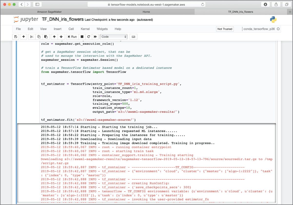
FIGURE 17.17 Using a notebook instance to create a training job
The training process is complete when you see lines similar to the following in the output:
After the training process is complete, Amazon SageMaker will automatically terminate the instance that was created to support the training. The model that was created will be saved to the awsml-sagemaker-results bucket, and the full path to the saved model is printed in the log messages. You can also view a list of trained models from the Models menu item of the AWS SageMaker management console (Figure 17.18) and access the model artifact file from there.
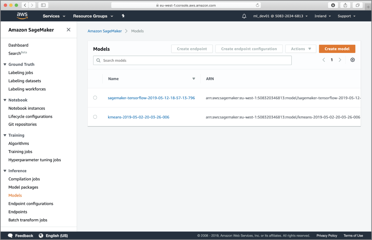
FIGURE 17.18 List of trained models
Now that you have a trained model, you can deploy the model to one or more dedicated prediction instances and then either create an HTTPS API endpoint for creating predictions on one item at a time, or create a batch transform job to obtain predictions on entire datasets. Using batch transforms is not covered in this chapter; however, you can find more information at https://docs.aws.amazon.com/sagemaker/latest/dg/ex1-batch-transform.html.
You can deploy models into prediction instances in several different ways, including using the AWS SageMaker Python SDK and the AWS management console. Regardless of the manner in which you choose to deploy the model, the process of deployment involves first creating an endpoint configuration object, and then using the endpoint configuration object to create the prediction instances and the HTTPS endpoint that can be used to get inferences from the deployed model. The endpoint configuration contains information on the location of the model file, the type and number of compute instances that the model will be deployed to, and the auto-scaling policy to be used to scale up the number of instances as needed.
If you use the high-level Amazon SageMaker Python SDK to deploy your model, the SDK provides a convenience function that takes care of creating the endpoint configuration, creation of compute resources, deployment of the model, and the creation of the HTTPS endpoint. If you use the lower-level AWS Boto Python SDK, you will need to perform the individual steps in sequence yourself. Keep in mind that prediction instances incur additional costs and are not automatically terminated after you have made predictions.
Execute the following code in an empty cell of the notebook to deploy the trained model to a single ML compute instance and create an HTTPS endpoint:
# create a prediction instancepredictor = tf_estimator.deploy(initial_instance:count=1,instance:type="ml.m4.xlarge")
This code assumes that the tf_estimator object has been created in the previous notebook cell where you trained the model. This is important because the deploy() function does not have an argument that lets you specify the path to the model file, but instead uses whatever model file is referenced within the tf_estimator object.
When you execute this code, Amazon SageMaker will take several minutes to create an endpoint configuration, create the compute instances, deploy your model onto the instances, and create an HTTPS endpoint. Once the prediction endpoint is created, the deploy() function will return an object of class TensorFlowPredictor, which provides a convenience function called predict() that can be used to make predictions from the HTTPS endpoint. The prediction endpoint is internet-facing and is secured using AWS Signature V4 authentication. You can access this endpoint in a variety of ways, including the AWS CLI, tools such as Postman, and the language-specific AWS SDKs. If you use the AWS CLI, or one of the AWS SDKs, authentication will be achieved behind the scenes for you. You can learn more about AWS Signature V4 at https://docs.aws.amazon.com/AmazonS3/latest/API/sig-v4-authenticating-requests.html.
If you want to expose the prediction endpoint as a service to your consumers, you can create an endpoint on an Amazon API Gateway instance and set up the Amazon API Gateway to execute an AWS Lambda function when it receives a request. You can then use one of the language-specific SDKs in the AWS Lambda function to interact with the prediction endpoint. The advantage of this approach is that your clients do not need to worry about AWS Signature V4 authentication, and an Amazon API Gateway can provide several features that are critical to managing the business-related aspects of a commercial API service such as credential management, credential rotation, support for OIDC, API versioning, and traffic management.
If you are using the AWS SageMaker Python SDK from a notebook instance, you can use the predict() function of the TensorFlowPredictor instance to make single predictions. Behind the scenes, the predict() function will use a temporary set of credentials associated with the IAM role assumed by the notebook instance to authenticate with the prediction endpoint. Execute the following code in an empty notebook cell to use the predict() function to predict the class of an Iris flower:
input_dict = {'sepal_length': 63.4,'sepal_width': 3.2,'petal_length': 4.5,'petal_width': 11.5 }# use the prediction endpoint to get a single predictionprediction = predictor.predict(input_dict)
You can use the Python print() function to examine the predictions:
To terminate the prediction instances and the associated HTTPS endpoint, you can, once again, use the high-level interface provided by the AWS SageMaker Python SDK. Execute the following code in a free notebook cell to terminate and deactivate the prediction endpoint:
You can also use the AWS SageMaker management console to view the list of active prediction endpoints, deactivate a prediction endpoint and terminate the associated prediction instances, and create new prediction endpoints from endpoint configurations.
- NOTE You can download the code files for this chapter from
www.wiley.com/go/machinelearningawscloudor from GitHub using the following URL:
Summary
- TensorFlow is a machine learning library created by Google, which was initially developed by the team at Google Brain for internal use, and then subsequently released as an open source project under the Apache license in November 2015.
- TensorFlow requires you to model your computation problem as a tree-like structure called a computation graph, made up of nodes and leaves.
- A constant leaf node (also known as a constant tensor) is a tensor whose value cannot be changed once it has been assigned.
- A variable leaf node (also known as a variable tensor) is a tensor whose value can be changed as the program executes.
- A placeholder leaf node (also known as a placeholder tensor) is a special node whose value is a tensor that you must feed into the graph when you evaluate the graph.
- Artificial neural networks (ANNs) are computing tools that were developed by Warren McCulloch and Walter Pitts in 1943, and their design is inspired by biological neural networks.
- The TensorFlow Python API is structured in a series of layers, with the topmost layer known as the Estimators API.
- Objects in the Estimators layer provide the ability to create entire neural networks with a single Python statement.
- You can train and deploy a machine learning model that uses the Estimators API on Amazon SageMaker.