
Chapter 2
Data Collection and Preprocessing
WHAT'S IN THIS CHAPTER
- Sources to obtain training data
- Techniques to explore data
- Techniques to impute missing values
- Feature engineering techniques
In the previous chapter, you were given a general overview of machine learning, and learned about the different types of machine learning systems. In this chapter you will learn to use NumPy, Pandas, and Scikit-learn to perform common feature engineering tasks.
- NOTE To follow along with this chapter ensure you have installed Anaconda Navigator and Jupyter Notebook as described in Appendix A.
You can download the code files for this chapter from
www.wiley.com/go/machinelearningawscloudor from GitHub using the following URL:
Machine Learning Datasets
Training a machine learning model requires high-quality data. In fact, lack of quality training data can result in the poor performance of models built using the best-known machine learning algorithms. Quality in this case refers to the ability of the training data to accurately capture the nuances of the underlying problem domain, and to be reasonably free of errors and omissions.
Some of the common sources for publicly available machine learning data are explored next.
Scikit-learn Datasets
The datasets package within Scikit-learn includes down-sampled versions of popular machine learning datasets such as the Iris, Boston, and Digits datasets. These datasets are often referred to as toy datasets. Scikit-learn provides functions to load the toy dataset into a dictionary-like object with the following attributes:
- DESCR: Returns a human-readable description of the dataset.
- data: Returns a NumPy array that contains the data for all the features.
- feature_names: Returns a NumPy array that contains the names of the features. Not all toy datasets support this attribute.
- target: Returns a NumPy array that contains the data for the target variable.
- target_names: Returns a NumPy array that contains the values of categorical target variables. The digits, Boston house prices, and diabetes datasets do not support this attribute.
The following snippet loads the toy version of the popular Iris dataset and explores the attributes of the dataset:
The list of toy datasets included with Scikit-learn are:
- Boston house prices dataset: This is a popular dataset used for building regression models. The toy version of this dataset can be loaded using the
load_boston()function. You can find the full version of this dataset athttps://archive.ics.uci.edu/ml/machine-learning-databases/housing/. - Iris plants dataset: This is a popular dataset used for building classification models. The toy version of this dataset can be loaded using the
load_iris()function. You can find the full version of this dataset athttps://archive.ics.uci.edu/ml/datasets/iris. - Onset of diabetes dataset: This is a popular dataset used for building regression models. The toy version of this dataset can be loaded using the
load_diabetes()function. You can find the full version of this dataset athttp://www4.stat.ncsu.edu/~boos/var.select/diabetes.html. - Handwritten digits dataset: This is a dataset of images of handwritten digits 0 to 9 and is used in classification tasks. The toy version of this dataset can be loaded using the
load_digits()function. You can find the full version of this dataset athttp://archive.ics.uci.edu/ml/datasets/Optical+Recognition+of+Handwritten+Digits. - Linnerud dataset: This is a dataset of exercise variables measured in middle-aged men and is used for multivariate regression. The toy version of this dataset can be loaded using the
load_linnerud()function. You can find the full version of this dataset athttps://rdrr.io/cran/mixOmics/man/linnerud.html. - Wine recognition dataset: This dataset is a result of chemical analysis performed on wines grown in Italy. It is used for classification tasks. The toy version of this dataset can be loaded using the
load_wine()function. You can find the full version of this dataset athttps://archive.ics.uci.edu/ml/machine-learning-databases/wine/. - Breast cancer dataset: This dataset describes the characteristics of cell nuclei of breast cancer tumors. It is used for classification tasks. The toy version of this dataset can be loaded using the
load_breast_cancer()function. You can find the full version of this dataset athttps://archive.ics.uci.edu/ml/datasets/Breast+Cancer+Wisconsin+(Diagnostic).
AWS Public Datasets
Amazon hosts a repository of public machine learning datasets that can be easily integrated into applications that are deployed onto AWS. The datasets are available as S3 buckets or EBS volumes. Datasets that are available in S3 buckets can be accessed using the AWS CLI, AWS SDKs, or the S3 HTTP query API. Datasets that are available in EBS volumes will need to be attached to an EC2 instance. Public datasets are available in the following categories:
- Biology: Includes popular datasets such as the Human Genome Project.
- Chemistry: Includes multiple versions of PubChem and other content. PubChem is a database of chemical molecules that can be accessed at
https://pubchem.ncbi.nlm.nih.gov. - Economics: Includes census data and other content.
- Encyclopedic: Includes Wikipedia content and other content.
You can browse the list of AWS public datasets at https://registry.opendata.aws.
Kaggle.com Datasets
Kaggle.com is a popular website that hosts machine learning competitions. Kaggle.com also contains a large number of datasets for general use that can be accessed at https://www.kaggle.com/datasets. In addition to the general-use datasets listed on the page, competitions on Kaggle.com also have their own datasets that can be accessed by taking part in the competition. The dataset files can be downloaded onto your local computer and can then be loaded into Pandas dataframes. You can get a list of current and past competitions at https://www.kaggle.com/competitions.
UCI Machine Learning Repository
The UCI machine learning repository is a public collection of over 450 datasets that is maintained by the Center for Machine Learning and Intelligent Systems at UC Irvine. It is one of the oldest sources of machine learning datasets and is often the go-to destination for beginners and experienced professionals alike. The datasets are contributed by the general public and vary in the level of preprocessing you will need to perform in order to use them for model building. The datasets can be downloaded onto your local computer and then processed using tools like Pandas and Scikit-learn. You can browse the complete list of datasets at https://archive.ics.uci.edu/ml/datasets.php.
A small selection of the most popular UCI machine learning repository datasets is also hosted at Kaggle.com and can be accessed at https://www.kaggle.com/uciml.
Data Preprocessing Techniques
In Chapter 1, you learned about the different types of machine learning systems and the general process in building a machine learning–based solution. It should come as no surprise that the performance of a machine learning system is heavily dependent on the quality of training data. In this section, you will learn some of the common ways in which data is prepared for machine learning models. The examples in this section will use datasets commonly found on the Internet and included with the downloads that accompany this lesson.
Obtaining an Overview of the Data
When building a machine learning model, one of the first things you will want to do is explore the data to get an overview of the variables and the target. This section uses the Titanic dataset in a Jupyter notebook with NumPy and Pandas. The dataset and the notebook files are included with the lesson's code resources.
The Titanic dataset is a very popular dataset that contains information on the demographic and ticket information of 1309 passengers on board the Titanic, with the goal being to predict which of the passengers were more likely to survive. The full dataset is available from the Department of BioStatistics at Vanderbilt University (https://biostat.mc.vanderbilt.edu/wiki/Main/DataSets). Versions of the titanic3 dataset are also available from several other sources, including a popular Kaggle.com competition titled Titanic: Machine Learning From Disaster (https://www.kaggle.com/c/titanic). The Kaggle version is included with the resources that accompany this chapter and has the benefit of being shuffled and pre-split into a training and validation set. The training set is contained in a file named train.csv and the validation set is test.csv.
The description of the attributes of the Kaggle version of the Titanic dataset are as follows:
- PassengerId: A text variable that acts as a row identifier.
- Survived: A Boolean variable that indicates if the person survived the disaster. 0 = No, 1 = Yes.
- Pclass: A categorical variable that indicates the ticket class. 1 = 1st class, 2 = 2nd class, 3 = 3rd class.
- Name: The name of the passenger.
- Sex: A categorical variable that indicates the sex of the passenger.
- Age: A numeric variable that indicates the age of the passenger.
- SibSp: A numeric variable that indicates the number of siblings/spouses traveling together.
- Parch: A numeric variable that indicates the number of parents and children traveling together.
- Ticket: A text variable containing the ticket number.
- Fare: A numeric variable that indicates the fare paid in Pre-1970 British pounds.
- Cabin: A textual variable that indicates the cabin number.
- Embarked: A categorical variable that indicates the port of embarkation. C = Cherbourg, Q = Queenstown, S = Southampton.
To load the Titanic training set from a CSV file located on your computer into a Pandas dataframe, use the following snippet:
The first thing to do is to get information on the number of rows and columns of the dataset. The shape attribute of the dataframe can be used to provide this information:
You can see that the dataframe has 891 rows and 12 columns (or attributes). The following snippet can be used to get the names of the columns:
One of the most common problems that data scientists have to deal with is that of missing values. Raw datasets often have missing values in one or more columns. There can be a number of reasons why the values are missing, ranging from human error to data simply being unavailable for that observation. When you load a CSV file into a Pandas dataframe, Pandas uses NaN as a marker to signify missing values. There are various ways to find out if a column in a dataframe contains missing values. One way is to use the info() function as illustrated in the following snippet:
Looking at the results of the info() function, it is clear that most columns have 891 values, whereas three columns—Age, Cabin, and Embarked—have less than 891 values. The use of the info() function to detect missing values only works if the value is truly missing in the CSV file, which means Pandas has been able to detect the missing value and substitute it with a NaN marker in the dataframe. If, however, the process by which the data was generated used a blank space, or a special character such as ! to represent a missing value, then Pandas will not automatically interpret these characters to represent missing data.
Another way to get information on missing values is to chain the output of the Pandas isnull() function with the sum() function. The isnull() function, when applied on a dataframe, returns a dataframe of boolean values that has the same dimensions as the original dataframe. Each position in the new dataframe has a value of True if the corresponding position in the original dataframe has a value of None or NaN. The sum() function, when applied to the new dataframe of boolean values, will returns a list with the number of values in each column that are True. The following snippet shows the result of chaining the isnull() and sum() functions to obtain the number of missing values in each column of the dataframe:
It is quite clear from the results that a significant number of Age and Cabin values are missing. We will look at ways to deal with missing values later in this chapter.
Sometimes the best way to get a feel for the data is to visually inspect the contents of the dataframe. You can use the head() function of the dataframe object to view the contents of the first few rows of the dataframe (Figure 2.1).
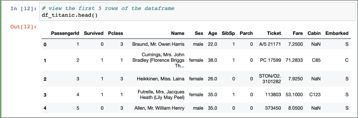
FIGURE 2.1 The head() function displays rows from the beginning of a Pandas dataframe.
If the number of columns is too many for Pandas to fit horizontally into a single line, then Pandas, by default, displays a subset of the columns of the dataframe. The subset consists of a few columns from the left of the dataframe, and a few from the right. Figure 2.2 illustrates the effect of using the head() function on a dataframe with 30 columns.
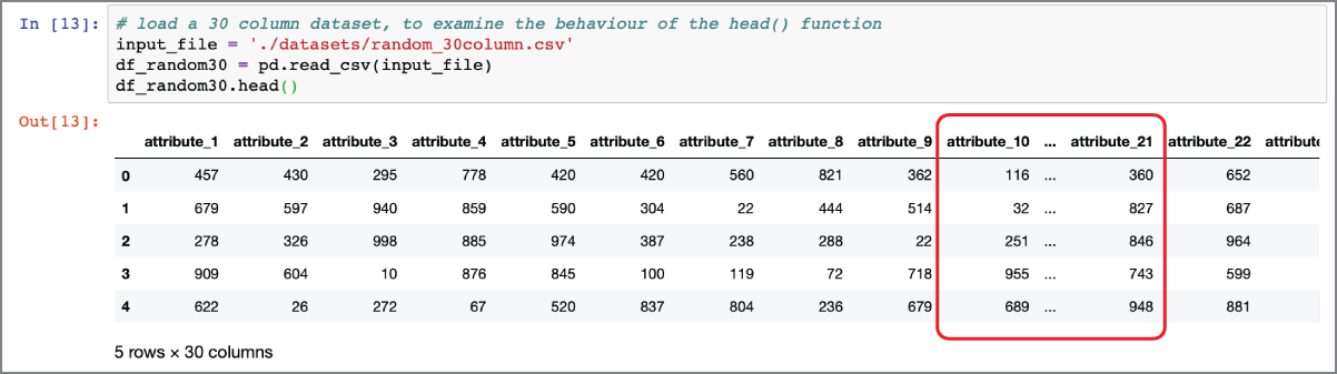
FIGURE 2.2 The head() function displays truncated data for large dataframes.
You can change the maximum number of columns that will be displayed by Pandas by setting the display.max_columns Pandas property. For example, the following snippet will ensure Pandas displays no more than four columns:
If you would like all columns to be displayed, set the value of display.max_columns to None:
Astute readers may have noticed that the PasengerId attribute of the Titanic dataset is a numeric row identifier and does not provide any useful input as far as model building is concerned. Every Pandas dataframe can have an index that contains a unique value for each row of the dataframe. By default, Pandas does not create an index for a dataframe; you can find out if a dataframe has an index by using the following snippet:
To make the PassengerId attribute the index of the df_titanic dataframe, use the following snippet:
If you were to examine the index of the dataframe after executing the set_index() function, you would see that the PassengerId attribute is now the index:
Figure 2.3 shows the results of applying the head() function to the df_titanic dataframe before and after the index has been set up.
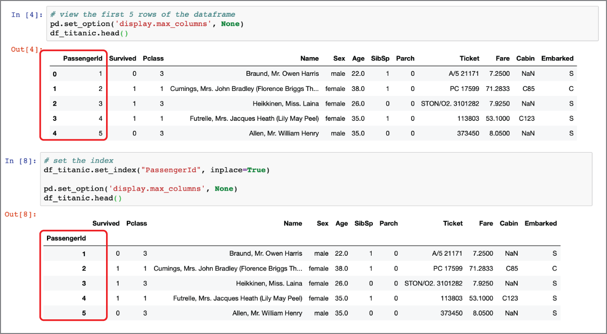
FIGURE 2.3 Impact of the set_index function on a dataframe
If you now use the shape attribute of the dataframe to get the number of rows and columns, you will notice that the number of columns is now reported as 11 instead of 12. This is illustrated in the following snippet:
You may have noticed that the Survived attribute is one of the 11 remaining attributes in the df_titanic dataframe after PassengerId has been used as the index. During the training process, you need to ensure you do not include the target attribute as one of the input features. There are various means by which you could ensure this, but perhaps the simplest option is to separate the feature variables and the target variables into separate dataframes. The following snippet will extract the Survived attribute from the df_titanic dataframe into a separate dataframe called df_titanic_target, and the 10 feature variables from the df_titanic dataframe into a separate dataframe called df_titanic_features:
The Survived attribute is a binary attribute in which a value of 1 implies that the individual survived. When the target that your machine learning model is trying to predict is categorical (binary or multi-class), it is useful to know the distribution of values in the training dataset per category. You can get the distribution of target values in this example by using the following snippet:
The value_counts() function can be used on numeric columns in addition to categorical columns. However, by default, the value_counts() function will not pick out NaN values. To have the value_counts() function include counts of NaN markers, include the dropna=false parameter as demonstrated in the following snippet:
If you prefer a visual representation of the distribution of target values, you can use the following snippet to create a histogram. The histogram is depicted in Figure 2.4.
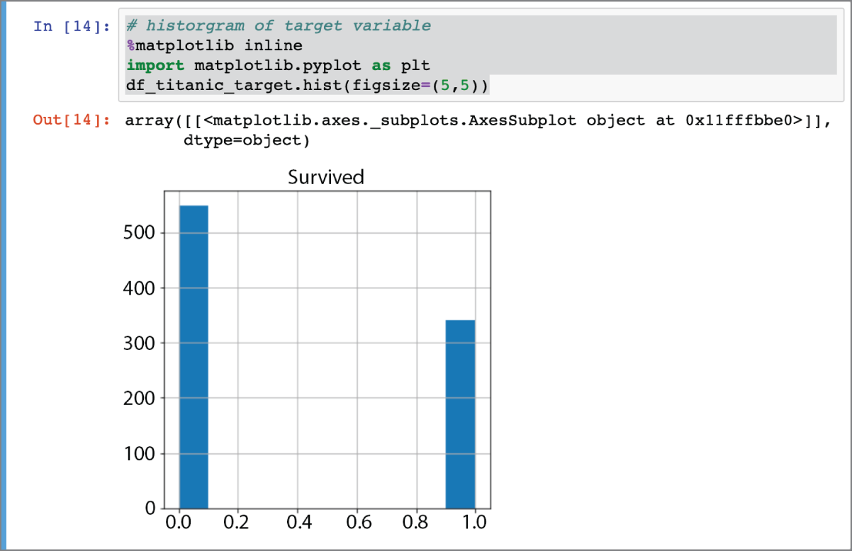
FIGURE 2.4 Distribution of values for the Survived attribute
In addition to a histogram of the target variables, it is also useful to use histograms to get an overview of the distribution of feature values. The hist() function provided by the Pandas dataframe object will only generate histograms for numeric values. The only numerical features in the Titanic dataset are Age, Fare, Pclass, Parch, and SibSp. The following snippet can be used to generate histograms of numeric features. The resulting feature histograms are depicted in Figure 2.5.
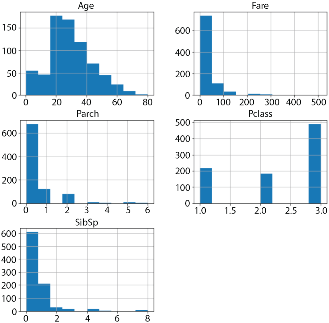
FIGURE 2.5 Histogram of numeric features
If you have a background in statistics, then you will be aware that the appearance of a histogram is influenced by the width of the bins. Data scientists often generate multiple histograms of the same variable with different bin widths to get a better understanding of the distribution of the data. The following snippet can be used to create a histogram of a single numeric attribute and specify the number of equal-width bins along the x-axis. Figure 2.6 depicts the histograms obtained by choosing a number of different bin widths for the same numerical feature.
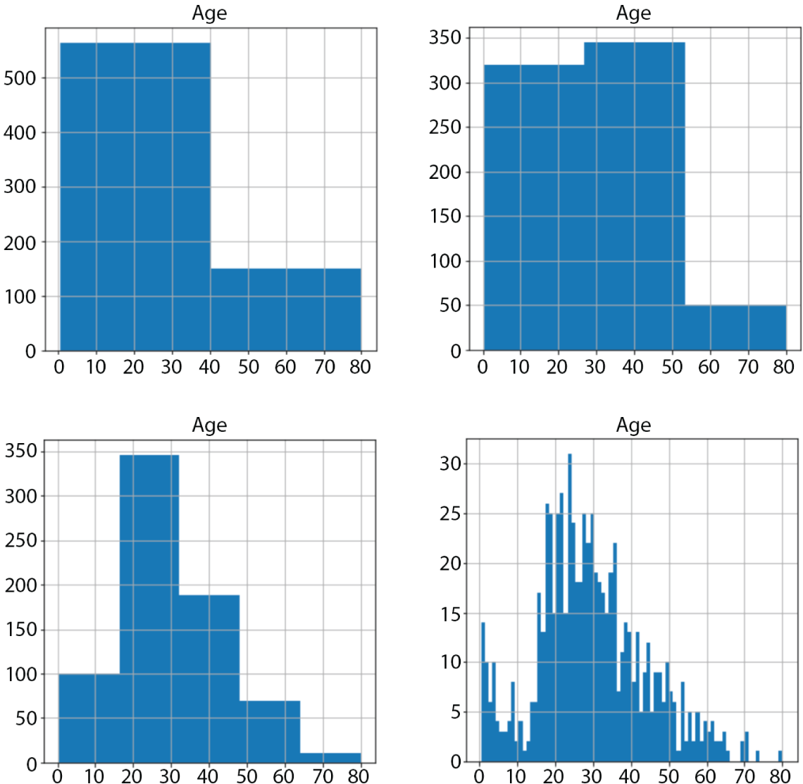
FIGURE 2.6 Histogram of numeric feature “Age” using different bin widths (2, 3, 5, 80)
Since the value_counts() function works on both numeric and categorical features, you could generate a histogram of a categorical feature by using the output of the value_counts() function. The following snippet demonstrates this approach on the Embarked categorical feature. The resulting histogram is depicted in Figure 2.7.
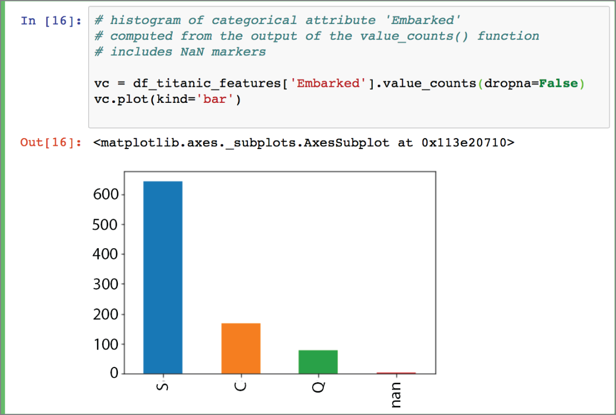
FIGURE 2.7 Histogram of categorical feature “Embarked”
In addition to information on the distribution of features and target variables, the statistical characteristics of these variables and the correlation between them can provide useful insights into the training data. Pandas provides a describe() function that can be used on dataframes to obtain statistical information on the numerical attributes within the dataframe. The following snippet shows the results of the describe() function on the df_titanic_features dataset:
Information provided by the describe() function includes the minimum value, maximum value, mean value, standard deviation, and the quartiles of each numerical feature. A quartile is a value below which a certain percent of observations can be found. For example, the first quartile is the value below which 25% of the observations can be found. The first quartile of the Age feature is 20.12, which means that 25% of the people captured by the dataset have ages less than 20 years. Information on quartiles and statistical characteristics of a feature is often represented using a box plot. Box plots are covered in Chapter 4; however, you can use the boxplot() function of the dataframe to create a box plot of all numeric features. The following snippet demonstrates the use of the boxplot() function. The resulting box plot is depicted in Figure 2.8.
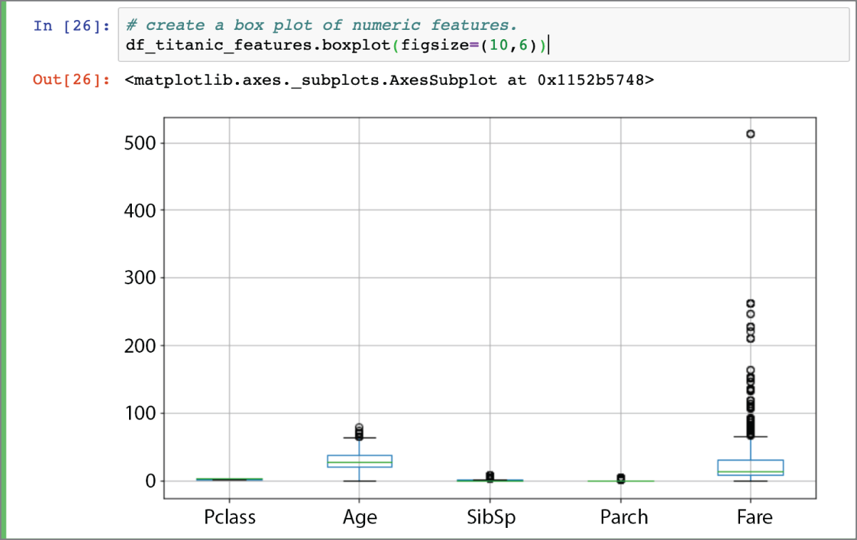
FIGURE 2.8 Box plot of numeric features
Information on the correlation between input features and the target can be helpful in picking out the best features from the data to use for model building and predictions. Information on the correlation between the features themselves can be helpful in reducing the number of features and the general risk of overfitting. Pandas provides a corr() function that can be used to compute Pearson's correlation coefficient between the columns of a dataframe. The results of applying the corr() function on the df_titanic dataframe is depicted in Figure 2.9.
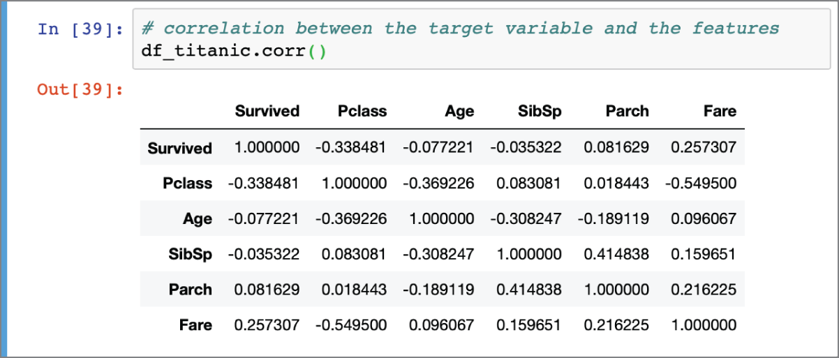
FIGURE 2.9 Linear correlation between numeric columns
It is important to note that Pearson's correlation coefficient will only detect linear correlation between variables. The corr() function allows you to choose from standard correlation coefficients such as Pearson, Kendall, and Spearman. You can find more information at https://pandas.pydata.org/pandas-docs/stable/reference/api/pandas.DataFrame.corr.html.
The following snippet lists the correlation between the numeric features and the target variable, sorted by descending value:
Computing correlation coefficients between pairs of attributes is not the only way to get information on the correlation between features. You can also create scatter plots between pairs of features to visualize their relationship. The following snippet uses the Pandas scatter_matrix() function to create scatter plots of all numeric features with each other. The resulting scatter plot is depicted in Figure 2.10.
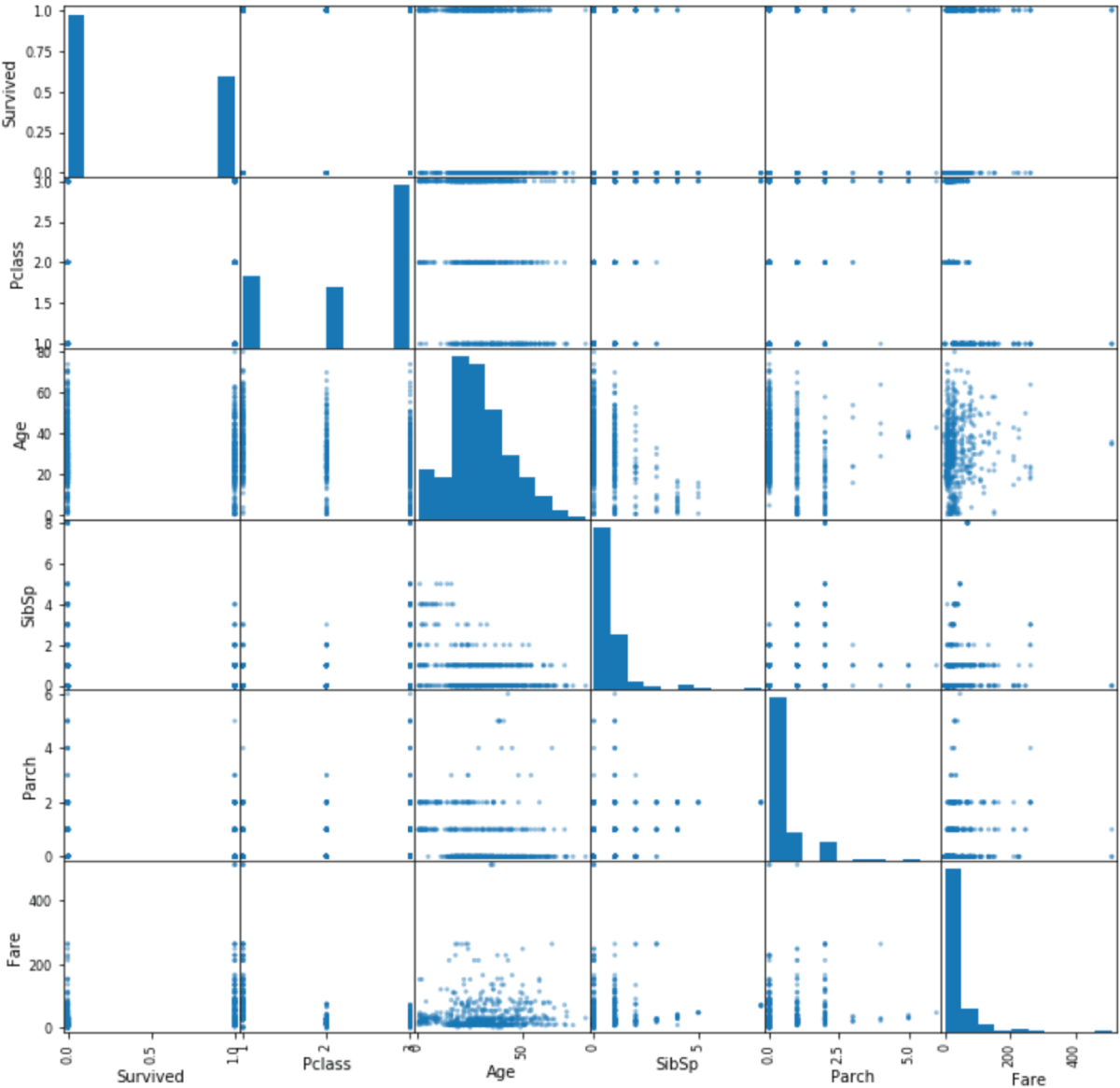
FIGURE 2.10 Matrix of scatter plots between pairs of numeric attributes
Handling Missing Values
In the previous section, you learned of techniques that can be used to explore the data. While exploring the Titanic dataset, you learned that the Age, Cabin, and Embarked classes have missing values. Age is a numeric feature, and we can use a box plot to get a quick overview of the statistical characteristics of the values that make up this feature using the following snippet. Figure 2.11 depicts a box plot of the Age feature variable.
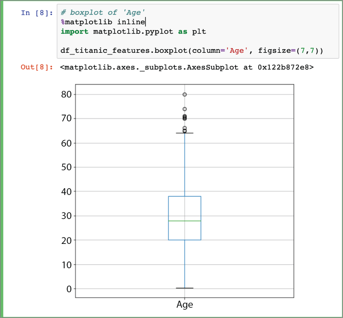
FIGURE 2.11 Box plot of the Age feature variable
The median value of the age, according to the box plot, is just under 30. Pandas provides the fillna() function that can be used to replace missing values with a new value. The following snippet uses the fillna() function to replace the missing values of the Age attribute with the median value:
- NOTE Although it is not demonstrated in this section, you must ensure that any feature engineering or imputation that is carried out on the training data is also carried out on the test data.
The Embarked attribute is categorical, and since the number of missing values is small (just 2), a reasonable approach is to substitute the missing values with the most frequently occurring value in the Embarked column. The following snippet uses the fillna() function to achieve this:
The Cabin attribute is also categorical but has a very large number of missing values (687). Using the same strategy that was used to impute missing values for the Embarked attribute will not work in this case as you will create a significant bias in the data. The best approach in this situation is to create a new boolean feature CabinIsKnown, which will have a value of True if the Cabin attribute is known, and False otherwise. You may be tempted to use the integer 1 to signify known cabin values and 0 to signify missing cabin values, but if you were to do this you would create an unintentional order in the data (1 being greater than 0), and this could influence the output of some models. The following snippet creates a new column called CabinIsKnown and drops the original Cabin column from the dataframe:
With the changes described in this section, you have imputed missing values where possible and created a new column in the dataframe. There should be no missing values in the dataframe, a new column called CabinIsKnown should be visible in the dataframe, and the Cabin column should have been deleted from the dataframe. All of this can be validated by executing the following snippet:
Creating New Features
If you observe the descriptions of the columns of the Titanic dataset, you will come across the SibSp and Parch columns. From the description of the dataset:
- SibSp: A numeric variable that indicates the number of siblings/spouses traveling together.
- Parch: A numeric variable that indicates the number of parents and children traveling together.
It may make sense to combine these values into a single numeric value that represents the size of the family traveling together. It is not possible to tell at this stage if the model will perform better with this additional synthesized feature, but having this new feature in the data will give you more options when it comes to building and evaluating models. The following snippet creates a new attribute in the dataframe called FamilySize, which is computed as the arithmetic sum of the SibSp and Parch attributes:
- NOTE Although it is not demonstrated in this section, you must ensure that any feature engineering that is carried out on the training data is also carried out on the test data.
The Age and Fare features are numeric and take on a range of values; it may be useful to bin the value of these features and create categorical features. During model building you may discover that the categorical (binned) values of Age and Fare provide better results. To create a new categorical feature called AgeCategory, you can use the Pandas cut() function as demonstrated in the following snippet:
Figure 2.12 depicts the output of the head() function on the df_titanic_features dataframe after the AgeCategory feature has been created.
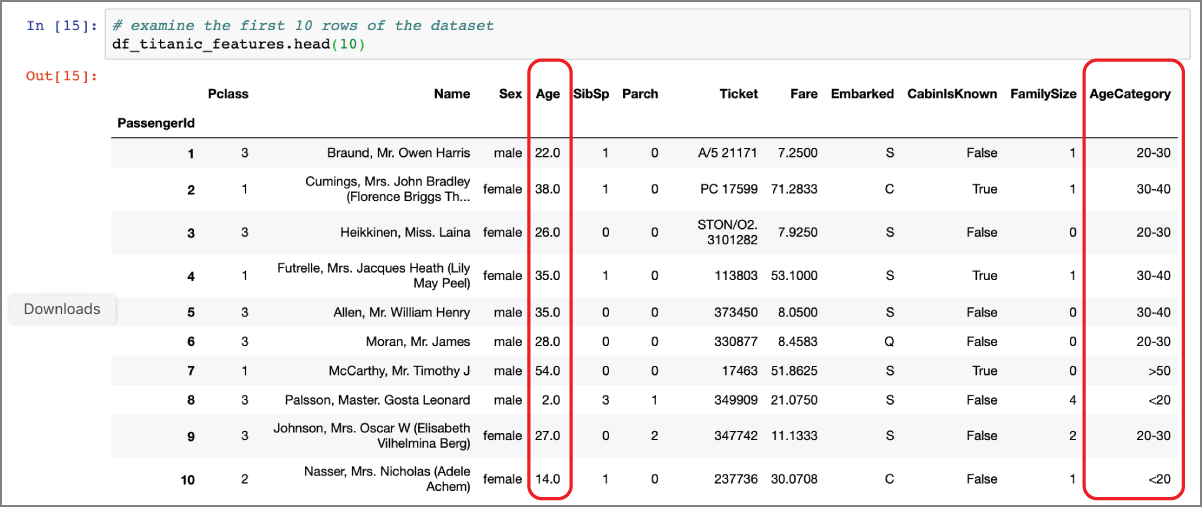
FIGURE 2.12 Dataframe with engineered feature AgeCategory
The cut() function has several parameters. In this example, the bins parameter contains a sequence of numbers that define the edges of the bins; the lowest and highest values are deliberately chosen to be outside the range of values observed in the Age feature. The labels parameter contains a list of strings that serve as the labels of the bins (and the values of the categorical feature that will be generated as a result of executing the cut() function). The include_lowest parameter is set to True to indicate that the first interval is left-inclusive. You can find information on the full list of parameters for the cut() function at https://pandas.pydata.org/pandas-docs/version/0.23.4/generated/pandas.cut.html.
There is no set formula to determine the correct number of bins and the widths of the bins. During the model-building process, you may find yourself experimenting with different binning strategies and pick the strategy that results in the best-performing model. If you want to split a continuous numeric variable into a categorical variable by using the quantiles as bin boundaries, you can use the Pandas qcut() function. The following snippet uses the qcut() function to create a new categorical feature called FareCategory using the quartiles as bin boundaries:
The second parameter, q=4, indicates that you want to use the quartiles as bin boundaries. Information on the qcut() function is available at https://pandas.pydata.org/pandas-docs/stable/reference/api/pandas.qcut.html.
Figure 2.13 depicts the output of the head() function on the df_titanic_features dataframe after the FareCategory feature has been created.
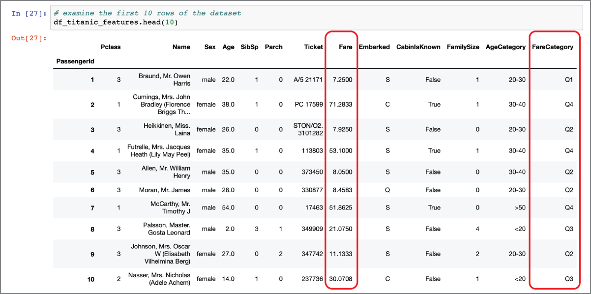
FIGURE 2.13 Dataframe with engineered feature FareCategory
Transforming Numeric Features
After having created the categorical features AgeCategory and FareCategory in the previous section, you may wish to drop the original Age and Fare attributes from the dataset. The decision to drop the original numerical values will largely depend on the type of model you are going to build.
When building a model with continuous numeric variables, you may need to transform numeric attributes. Several machine learning models converge faster and work better when the values of numeric attributes are small and have a distribution that is close to a standard normal distribution with mean 0 and variance 1.
Normalization and standardization are the two most common types of transformations performed on numerical attributes. The result of normalizing a feature is that the values of the feature will be scaled to fall within 0 and 1. The result of standardizing a feature is that the distribution of the new values will have a mean of 0 and a standard deviation of 1, but the range of the standardized values is not guaranteed to be between 0 and 1. Standardization is used when the model you want to build assumes the feature variables have a Gaussian distribution. Normalization is often used with neural network models, which require inputs to lie within the range [0, 1].
Scikit-learn provides a number of classes to assist in scaling numeric attributes. The MinMaxScaler class is commonly used for normalizing features, and the StandardScaler class is commonly used for standardization. The following snippet creates two new columns, NormalizedAge and StandardizedAge, in the df_titanic_features dataframe. Figure 2.14 compares the histogram of the Age, NormalizedAge, and StandardizedAge features:
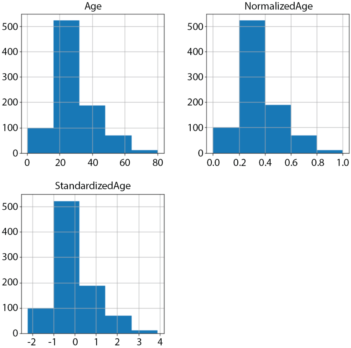
FIGURE 2.14 Histogram of Age, NormalizedAge, and StandardizedAge
One-Hot Encoding Categorical Features
The final topic that we will look at in this chapter will be converting categorical features into numeric features using one-hot encoding. You may be wondering why you would want to convert categorical features to numeric, especially since a previous section in this chapter has discussed techniques to do the opposite—converting numeric features into categorical.
Not all machine learning algorithms can deal with categorical data. One-hot encoding is a technique that converts a categorical feature into a number of binary numeric features, one per category. For example, linear regression and logistic regression are only capable of using numeric features. Algorithms like XGBoost and random forests are capable of using categorical features without any problems.
Pandas provides the get_dummies() function to help with one-hot encoding. The following snippet will convert the categorical features Sex, Embarked, CabinIsKnown, AgeCategory, and FareCategory into binary numeric features and list the columns of the dataframe:
As can be seen from the preceding snippet, the original categorical attributes are no longer present in the df_titanic_features dataframe; however, a number of new columns have been added. To understand how Pandas has created the additional columns, consider the Sex categorical attribute. This attribute has two values: male, and female. To convert this categorical attribute into a binary numeric attribute, Pandas has created two new columns in the dataframe called Sex_male and Sex_female. Other categorical attributes such as Embarked, CabinIsKnown, etc. have been processed using a similar approach. The following snippet lists the values of the Sex_male and Sex_female columns for the first five rows of the dataframe:
Astute readers may notice that since the values taken by the Sex attribute in the original df_titanic_features dataset is either male or female, you don't need both Sex_male and Sex_female attributes because you can infer one from the other. These two attributes have a very strong negative correlation of –1.0 and you should not use both of them as inputs to a machine learning model. The following snippet demonstrates the strong negative correlation between the two attributes:
The situation is similar with the CabinIsKnown_False and CabinIsKnown_True features. The following snippet drops the Sex_female and CabinIsKnown_False attributes along with non-numeric attributes Name and Ticket to arrive at a dataframe that contains only numeric attributes:
If you compute the correlation between the target attribute Survived and these numeric features, you will see a significantly better correlation than achieved earlier in this chapter prior to feature engineering. The following snippet demonstrates this:
Note the particularly strong negative correlation between the chances of survival and Sex_male, and the strong positive and negative correlation with FareCategory_Q4 and FareCategory_Q1, respectively.
Feature engineering is the most laborious and time-consuming aspect of data science, and there is no set formula that can be applied to a given situation. In this chapter you have learned some of the techniques that can be used to explore data, impute missing values, and engineer features.
- NOTE To follow along with this chapter ensure you have installed Anaconda Navigator and Jupyter Notebook as described in Appendix A.
You can download the code files for this chapter from
www.wiley.com/go/machinelearningawscloudor from GitHub using the following URL:
Summary
- A number of sources of datasets can be used to create machine learning models. Some of the popular sources are the UCI machine learning repository,
Kaggle.com, and AWS public datasets. - Scikit-learn includes subsampled versions of popular datasets that are often used by beginners.
- Pandas provides the
read_csv()function that allows you to load a CSV file into a dataframe. - You can use the Pandas
isnull()andsum()functions together to obtain the number of missing values in each column of a dataframe. - The
hist()function exposed by the Pandas dataframe object will only generate histograms for numeric values. - Pandas provides a
describe()function that can be used on dataframes to obtain statistical information on the numerical attributes within the dataframe. - Pandas provides a
corr()function that can be used to compute Pearson's correlation coefficient between the columns of a dataframe. - You can also create scatter plots between pairs of features to visualize their relationship.
- Pandas provides the
fillna()function that can be used to replace missing values with a new value.