
Chapter 1
Introduction to Machine Learning
WHAT'S IN THIS CHAPTER
- Introduction to the basics of machine learning
- Tools commonly used by data scientists
- Applications of machine learning
- Types of machine learning systems
- Comparison between a traditional and a machine learning system
Hello and welcome to the exciting world of machine learning with Amazon Web Services (AWS). If you have never heard of machine learning until now, you may be tempted to think that it is a recent innovation in computer science that will result in sentient computer programs, significantly more intelligent than humans, that will one day make humans obsolete. There is very little truth in that idea of machine learning. For starters, it is not a recent development. For decades computer scientists have been researching ways to make computers more intelligent, attempting to find ways to teach computers to reason and to make decisions, generalizations, and predictions much like humans do.
Machine learning specifically deals with the problem of creating computer programs that can generalize and predict information reliably, quickly, and with accuracy resembling what a human would do with similar information. Building machine learning models can require a lot of processing power and storage space, and until recently was only possible to implement in very large companies or in academic institutions. Recent advances in storage, processor speeds, GPU technology, and the ability to rapidly create new virtual computing resources in the cloud have finally provided the processing power require to build and deploy machine learning systems at scale, and get results in real time.
Another factor that has contributed to the recent increase in machine learning applications is the availability of excellent tools such as Pandas, Matplotlib, TensorFlow, Scikit-learn, PyTorch, and Jupyter Notebook, which have made it possible for newcomers to start building real-world machine learning applications without having to delve into the complex underlying mathematical concepts.
Cloud computing as we know it today was born in 2006 when Amazon launched its Elastic Compute Cloud (EC2) service. Soon after in 2008, Microsoft launched its Azure service. This was followed by competing offers from other players, including Rackspace, Google, Oracle, and Apple. Building and deploying machine learning applications in the cloud is extremely popular. Most major cloud providers offer services to build and deploy some kind of machine learning applications.
You can find more information on the basics of cloud computing and Amazon Web Services in Chapters 6 and 7. In this chapter you will learn about what machine learning is, how machine learning systems are classified, and examples of real-world applications of machine learning.
What Is Machine Learning?
Machine learning is a discipline within Artificial Intelligence (AI) that deals with creating algorithms that learn from data. Machine learning traces its roots to a computer program created in 1959 by the computer scientist Arthur Samuel while he was working for IBM. Samuel's program could play a game of checkers and was based on assigning each position on the board a score that indicated the likelihood of leading toward winning the game. The positional scores were refined by having the program play against itself, and with each iteration the performance of the program improved. The program was, in effect, learning from experience, and the field of machine learning was born.
A machine learning system can be described as a set of algorithms based on mathematical principles that can mine data to find patterns in the data and then make predictions on new data as it is encountered. Rule-based systems can also make predictions on new data; however, rule-based systems and machine learning systems are not the same. A rule-based system requires a human to find patterns in the data and define a set of rules that can be applied by the algorithm. The rules are typically a series of if-then-else statements that are executed in a specific sequence. A machine learning system, on the other hand, discovers its own patterns and can continue to learn with each new prediction on unseen data.
Tools Commonly Used by Data Scientists
In this section you will learn about some of the tools commonly used by data scientists to build machine learning solutions. Most machine learning scientists use one of two programming languages: Python or R. R is a language commonly used by statisticians. While R has historically been the more popular choice, availability of machine learning–specific libraries in Python have made Python the more popular choice today. This book uses Python 3.6.5 and the rest of this section will focus on the most popular machine learning tools for Python:
- Jupyter Notebook: This is a very popular web-based interactive development environment for data science projects. A notebook combines code, execution results, and visualization results all in a single document. Jupyter Notebook is a successor to an older project called IPython Notebook. You can find out more about Jupyter Notebook at
http://jupyter.org. Appendix A contains instructions on installing Anaconda Navigator and setting up Jupyter Notebook on your own computer. - Anaconda Navigator: This is a commonly used package manager for data scientists. It allows users to conveniently install and manage Python and R libraries and quickly switch between different sets of libraries and language combinations. It also includes popular tools such as Jupyter Notebook, Spyder Python IDE, and R Studio. You can find more information on Anaconda at
https://www.anaconda.com. - Scikit-learn: This is a Python library that provides implementations of several machine learning algorithms for classification, regression, and clustering applications. It also provides powerful data preprocessing and dimensionality reduction capabilities. You can find more information on Scikit-learn at
https://www.scikit-learn.org. - NumPy: This is a Python library that is commonly used for scientific computing applications. It contains several useful operations such as random number generation and Fourier transforms. The most popular NumPy features for data scientists are N-dimensional data arrays (known as ndarrays) and functions that manipulate these arrays. NumPy ndarrays allow you to perform vector and matrix operations on arrays, which is significantly faster than using loops to perform element-wise mathematical operations. You can find more information on NumPy at
https://www.numpy.org. - Pandas: This is a Python library that provides a number of tools for data analysis. Pandas builds upon the NumPy ndarray and provides two objects that are frequently used by data scientists: the Series and the DataFrame. You can find more information on Pandas at
https://pandas.pydata.org. - Matplotlib: This is a popular 2D plotting library. It is used by data scientists for data visualization tasks. You can find more information on Matplotlib at
https://matplotlib.org. - Pillow: This is a library that provides a variety of functions to load, save, and manipulate digital images. It is used when the machine learning system needs to work with images. You can find more information on Pillow
athttps://python-pillow.org. - TensorFlow: This is Python library for numerical computation. It was developed by Google and eventually released as an open source project in 2015. TensorFlow is commonly used to build deep-learning systems. It uses a unique computation-graph–based approach and requires users to build a computation graph where each node in the graph represents a mathematical operation and the connections between the nodes represent data (tensors). You can find more information on TensorFlow at
https://www.tensorflow.org. - PyTorch: This is another popular Python library for training and using deep-learning networks. It was built by Facebook, and many newcomers find it easier to work with than TensorFlow. You can find more information on PyTorch at
https://pytorch.org.
Common Terminology
In this section we will examine some of the common machine learning–specific terminology that you are likely to encounter. While this list is not exhaustive, it should be useful to someone looking to get started:
- Machine learning model: This is the algorithm that is used to make predictions on data. It can also be thought of as a function that can be applied to the input data to arrive at the output predictions. The machine learning algorithm often has a set of parameters associated with it that influence its behavior, and these parameters are determined by a process known as training.
- Data acquisition: The process of gathering the data needed to train a machine learning model. This could include activities ranging from downloading ready-to-use CSV files to scraping the web for data.
- Input variables: These are the inputs that your machine learning model uses to generate its prediction. A collection of N input variables are generally denoted by lowercase xi with i = 1, 2, 3, …N. Input variables are also known as features.
- Feature engineering: This is the process of selecting the best set of input variables and often involves modifying the original input variables in creative ways to come up with new variables that are more meaningful in the context of the problem domain. Feature engineering is predominantly a manual task.
- Target variable: This is the value you are trying to predict and is generally denoted by a lowercase y. When you are training your model, you have a number of training samples for which you know the expected value of the target variable. The individual values of the target variable for N samples are often referred to as yi with i = 1, 2, …N.
- Training data: A set of data that contains all the input features as well as any engineered features and is used to train the model. For each item in the set, the value of the target variable is known.
- Test data: A set of data that contains all the input features (including engineered features), as well as the values of the target variable. This set is not used while training the model, but instead is used to measure the accuracy of the model's predictions.
- Regression: A statistical technique that attempts to find a mathematical relationship between a dependent variable and a set of independent variables. The dependent variable is usually called the target, and the independent variables are called the features.
- Classification: The task of using an algorithm to assign observations a label from a fixed set of predefined labels.
- Linear regression: A statistical technique that attempts to fit a straight line, plane, or hyperplane to a set of data points. Linear regression is commonly used to create machine learning models that can be used to predict continuous numeric values (such as height, width, age, etc.)
- Logistic regression: A statistical technique that uses the output of linear regression and converts it to a probability between 0 and 1 using a sigmoid function. Logistic regression is commonly used to create machine learning models that can predict class-wise probabilities. For example, the probability that a person will develop an illness later in life, or the probability that an applicant will default on a loan payment.
- Decision tree: A tree-like data structure that can be used for classification and prediction problems. Each node in the tree represents a condition, and each leaf represents a decision. Building a decision tree model involves examining the training data and determining the node structure that achieves the most accurate results.
- Error function: A mathematical function that takes as input the predicted and actual values and returns a numerical measure that captures the prediction error. The goal of the training function is to minimize the error function.
- Neural networks: A machine learning model that mimics the structure of the human brain. A neural network consists of multiple interconnected nodes, organized into distinct layers—the input layer, the in-between layers (also known as the hidden layers), and the output layer. Nodes are commonly known as neurons. The number of neurons in the input layer correspond to the number of input features, and the number of neurons in the output layer correspond to the number of classes that are being predicted/classified.
- Deep learning: A branch of machine learning that utilizes multi-layer neural networks with a large number of nodes in each layer. It is also quite common for deep-learning models to use multiple deep neural networks in parallel.
Real-World Applications of Machine Learning
Machine learning is transforming business across several industries at an unprecedented rate. In this section you will learn about some of the applications of machine learning–based solutions:
- Fraud detection: Machine learning is commonly used in banks and financial institutions to make a decision on the overall risk associated with a payment instruction. Payments in this context include money transfers and purchases (payments to providers) using cards. The risk decision is based on several factors, including the transactional history. If the risk is low, the transaction is allowed to proceed. If the risk is too high, the transaction is declined. If the risk is deemed to lie in an acceptable threshold, the customer may be asked to perform some form of step-up authentication to allow the transaction to proceed.
- Credit scoring: Whenever a customer applies for a credit product such as a loan or credit card, a machine learning system computes a score to indicate the overall risk of the customer not being able to repay the loan.
- Insurance premium calculation: Machine learning systems are commonly used to compute the insurance premium that is quoted to customers when they apply to purchase an insurance product.
- Behavioral biometrics: Machine learning systems can be trained to build a profile of users based on the manner in which they use a website or a mobile application. Specifically, such systems create a profile of the user based on analyzing information on the location of the user at the time when the system was accessed, the time of the day, the precise click locations on a page, the length of time spent on a page, the speed at which the mouse is moved across the page, etc. Once the system has been trained, it can be used to provide real-time information on the likelihood that someone is impersonating a customer.
- Product recommendations: Machine learning systems are commonly used by online retailers (such as Amazon) to provide a list of recommendations to customers based on their purchase history. These systems can even predict when a customer is likely to run out of groceries or consumables and send reminders to order the item.
- Churn prediction: Machine learning systems are commonly used to predict which customers are likely to cancel their subscription to a product or service in the next few days. This information gives businesses an opportunity to try to retain the customer by offering a promotion.
- Music and video recommendations: Online content providers such as Netflix and Spotify use machine learning systems to build complex recommendation engines that analyze the movies and songs you listen to and provide recommendations on other content that you may like.
Types of Machine Learning Systems
There are several different types of machine learning systems today. The classification of a machine learning system is usually based on the manner in which the system is trained and the manner in which the system can make predictions. Machine learning systems are classified as follows:
- Supervised Learning
- Unsupervised Learning
- Semi-supervised Learning
- Reinforcement Learning
- Batch Learning
- Incremental Learning
- Instance-based Learning
- Model-based Learning
These labels are not mutually exclusive; it is quite common to come across a machine learning system that falls into multiple categories. For example, a system that uses behavioral usage data to detect potential fraudsters on a banking website could be classified as a supervised model–based machine learning system. Let's examine these classification labels in more detail.
Supervised Learning
Supervised learning refers to the training phase of the machine learning system. During the supervised training phase, the machine learning algorithm is presented with sets of training data. Each set consists of inputs that the algorithm should use to make predictions as well as the desired (correct) result (Figure 1.1).
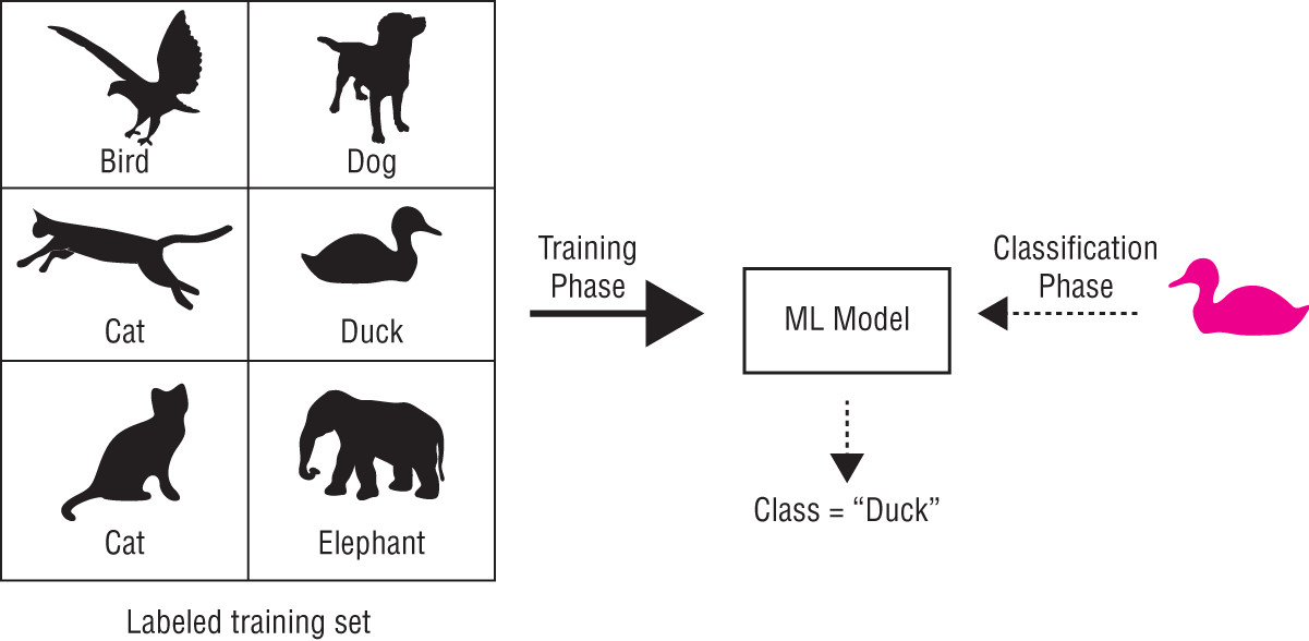
FIGURE 1.1 Supervised learning
Training consists of iterating over each set, presenting the inputs to the algorithm, and comparing the output of the algorithm with the desired result. The difference between the actual output and the desired output is used to adjust parameters of the algorithm so as make the output of the algorithm closer to (or equal to) the desired output.
Human supervision is typically needed to define the desired output for each input in the training set. Once the algorithm has learned to make predictions on the training set, it can be used to make predictions on data it has not previously encountered.
Most real-world machine learning applications are trained using supervised learning techniques. Some applications of supervised learning are:
- Finding objects in digital images
- Spam filtering
- Predicting the possibility of developing a medical condition based on lifestyle factors
- Predicting the likelihood of a financial transaction being fraudulent
- Predicting the price of property
- Recommending a product to a customer based on historical purchasing data
- A music streaming servicing suggesting a song to a customer based on what the customer has been listening to
Unsupervised Learning
Unsupervised learning also refers to the training phase of a machine learning system. However, unlike supervised learning, the algorithm is not given any information on the class/category associated with each item in the training set. Unsupervised learning algorithms are used when you want to discover new patterns in existing data. Unsupervised learning algorithms fall into two main categories:
- Clustering These algorithms group the input data into a number of clusters based on patterns in the data. Visualizing these clusters can give you helpful insight into your data. Figure 1.2 shows the results of a clustering algorithm applied to the data on the heights and ages of children under 6 years of age. Some of the most popular clustering algorithms are k-means clustering, and Hierarchical Cluster Analysis (HCA).
- Dimensionality reduction These algorithms are used to combine a large number of input features into a smaller number of features without losing too much information. Typically, the features that are combined have a high degree of correlation with each other. Dimensionality reduction reduces the number of input features and therefore the risk of overfitting; it also reduces the computational complexity of a machine learning model. Some examples of algorithms in this category are Principal Component Analysis (PCA), Linear Discriminant Analysis (LDA), and Autoencoding. Dimensionality reduction is often used when the number of features in a dataset is too large for a data scientist to meaningfully analyze.
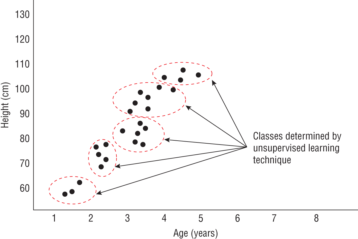
FIGURE 1.2 Clustering technique used to find patterns in the data
Semi-Supervised Learning
Semi-supervised learning is a mix of both supervised and unsupervised learning. In many situations it is practically impossible for a data scientist to label millions of samples for a supervised learning approach; however, the data scientist is already aware that there are known classifications in the data. In such a case, the data scientist labels a small portion of the data to indicate what the known classifications are, and the algorithm then processes the unlabeled data to better define the boundaries between these classes as well as potentially discover new classes altogether. Figure 1.3 depicts the results of applying semi-supervised learning to the same data on the heights and ages of children under 6 years of age, with some of the samples labeled to indicate the level of education.
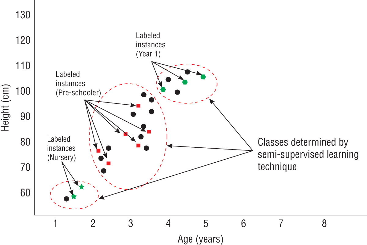
FIGURE 1.3 Semi-supervised learning
Real-world problems that involve extremely large datasets use this approach. Applications include speech recognition, natural language parsing, and gene sequencing.
A distinct advantage of semi-supervised learning is that it is less prone to labeling bias than supervised learning. This is because a data scientist is only labeling a small portion of the data, and the effects of any personal labeling bias introduced by the scientist can be corrected by the unsupervised learning part of the algorithm based on the sheer number of unlabeled samples it will process.
Semi-supervised learning algorithms make an assumption that the decision boundaries are geometrically simple; in other words, points that are close to each other are actually related in some way.
Reinforcement Learning
Reinforcement learning is a computational approach that attempts to learn using techniques similar to how humans learn: by interacting with their environment and associating positive and negative rewards with different actions. For instance, human beings have learned over time that touching a fire is a bad thing; however, using the same fire for cooking or providing warmth is a good thing. Therefore when we come across a fire we use it in positive ways.
A reinforcement learning–based system is typically called an agent and has a number of fixed actions that it can take at any given point in time, and with each action is an associated reward or penalty. The goal of the system is to maximize the cumulative reward over a series of actions. The knowledge gained by the agent is represented as a set of policies that dictate the actions that must be taken when the agent encounters a given situation. Reinforcement learning–based systems are used with two types of tasks:
- Episodic tasks: This is when the problem has a finite end point, such as winning a game.
- Continuous tasks: This is when the problem has no end point, such as maximizing the value of a stock portfolio.
Reinforcement learning algorithms often work in an environment where the results of choices are often delayed. Consider, for instance, an automated stock trading bot. It has several real-time inputs, manages several stocks, and can take one of three given actions at any point in time: buy a stock, sell a stock, or hold on to the stock. The result of several buy and sell decisions could be an eventual increase in the value of the portfolio (reward), or decrease in the value of the portfolio (penalty).
The bot does not know beforehand if taking a given action will result in reward or penalty. The bot must also incorporate a delay mechanism and not attempt to gauge reward/penalty immediately after making a transaction. The goal of the bot is to maximize the number of rewards.
In time the bot would have learned of trading strategies (policies) that it can apply in different situations. Reinforcement learning coupled with deep learning neural networks is a hotly researched topic among machine learning scientists.
Batch Learning
Batch learning refers to the practice of training a machine learning model on the entire dataset before using the model to make predictions. A batch learning system is unable to learn incrementally from new data it encounters in the future. If you have some new additional data that you want to use to train a batch learning system, you need to create a new model on all the data you have used previously plus the new additional data, and replace the older version of the model with this newly trained one.
Batch learning systems work in two distinct modes: learning and prediction. In learning mode the system is in training and cannot be used to make predictions. In prediction mode the system does not learn from observations.
The training process can be quite lengthy, and require several weeks and several computing resources. You also need to retain all training data in the event that you need to train a new version of the model. This can be problematic if the training data is large and requires several gigabytes of storage.
Incremental Learning
Incremental learning, also known as online learning, refers to the practice of training a machine learning model continuously using small batches of data and incrementally improving the performance of the model. The size of a mini batch can range from a single item to several hundred items. Incremental learning is useful in scenarios where the training data is available in small chunks over a period of time, or the training data is too large to fit in memory at once. The aim of incremental learning is to not have to retrain the model with all the previous training data; instead, the model's parameters (knowledge) are updated by a small increment with each new mini batch that it encounters. Incremental learning is often applied to real-time streaming data or very large datasets.
Instance-based Learning
Instance-based learning systems make a prediction on new unseen data by picking the closest instance from instances in the training dataset. In effect the machine learning system memorizes the training dataset and prediction is simply a matter of finding the closest matching item. The training phase of instance-based learning systems involves organizing all the training data in an appropriate data structure so that finding the closest item during the prediction phase will be quicker. There is little (if any) model tuning involved, although some level of preprocessing may have been performed on the training data before presenting it to the machine learning system.
The advantage of an instance-based learning system is that both training and prediction are relatively quick, and adding more items to the training set will generally improve the accuracy of the system. It is important to note that the prediction from an instance-based system will be an instance that exists in the training set. For example, consider an instance-based machine learning system that predicts the shoe size of an individual given a height and weight value as input. Let's assume this system is trained using a training set of 100 items, where each item consists of a height, weight, and shoe size value.
If this instance-based machine learning system were to be used to predict the shoe size for a new individual given a height and weight of the new individual as input values, the predicted shoe size would be the value of the closest matching item in the training set. To put it another way, the machine learning system would never output a shoe size that was not in the training set to start with.
Model-based Learning
Model-based learning systems attempt to build a mathematical, hierarchical, or graph-based model that models the relationships between the inputs and the output. Prediction involves solving the model to arrive at the result. Most machine learning algorithms fall in this category.
While model-based systems require more time to build, the size of the model itself is a fraction of the size of the training data, and the training data need not be retained (or presented to the model) in order to get a prediction. For example, a model built from a training dataset of over a million items could be stored in a small five-element vector.
The Traditional Versus the Machine Learning Approach
As humans, all of us are familiar with the concept of learning. Learning takes two major forms: memorization and understanding. There is a clear difference between memorizing your password and learning to drive a car. The latter involves understanding how the vehicle works, and how to react in different situations on the road. You do not memorize the exact sequence of activities you need to perform to drive between your home and your place of work; instead, you apply the understanding you have gained while assessing the situation on the road.
The capabilities of machine learning algorithms are not as sophisticated as human learning. Machines do not have the capability to understand and reason; however, they can predict and generalize, and they are capable of processing data much faster than humans. In this section you will examine a hypothetical situation and understand how a machine learning system can be applied to solve the problem at hand.
Imagine you have been hired by the credit cards team at a bank and tasked with creating a solution to offer a new credit card product to customers. Eligible customers can, under this new product, get cards with credit limits up to $25,000 at low interest rates. The bank would like to keep its losses to a minimum and requires that the credit card only be offered to customers who are likely to pay the money back to the bank.
To start with, you decide to create a new application form that customers will need to fill out to apply for this credit card. On the application form, you ask for the following information:
- Name
- Age
- Sex
- Number of years lived at current address
- Number of addresses in the last 5 years
- Number of credit cards held with other banks
- Total amount of loan (excluding mortgage)
- Total income after tax
- Estimated regular monthly outgoings
- Total monthly repayments
- Homeowner status
- Marital status
- Number of dependents in the household
In a real-world scenario you would ask for a lot more information and would also use a credit scoring company to provide the applicant's credit rating, but for the purposes of this example this list will do. Let's also assume that the mechanism to allow customers to apply for the credit card is available on the bank's website, and data from all application forms is available in a table in a SQL database within the bank.
When the product is launched, your bank expects it to be popular with customers and you need to have a plan in place to process a large number of applications each week. It is also crucial for your bank to remain competitive in the credit card space, and therefore you cannot keep applicants waiting for weeks to find out the outcome of a credit card application. You need to ensure that the bank's standard terms of service apply to your new product and therefore at least 51% of all credit applications need to be decided within a few minutes of the application being received by the bank.
Clearly, it is not cost effective to a hire few hundred analysts to scrutinize each loan application and make the necessary checks to arrive at a decision. You have two choices before you:
- You can build a rule-based decisioning system
- You can build a machine learning system
Let's first examine how a rule-based system could be used to help with this problem.
A Rule-based Decision System
Faced with the prospect of choosing between an easy-to-understand rule-based approach, and a somewhat unknown, black-box machine learning system, you decide to go with a rule-based decision system.
The business rules themselves are to be stored in a database, and the business logic to apply the rules to a loan application will be encapsulated into a server-side application. You plan to have a cluster of these servers that can be scaled up as necessary to deal with increased volumes. Figure 1.4 depicts the architecture of the proposed system.
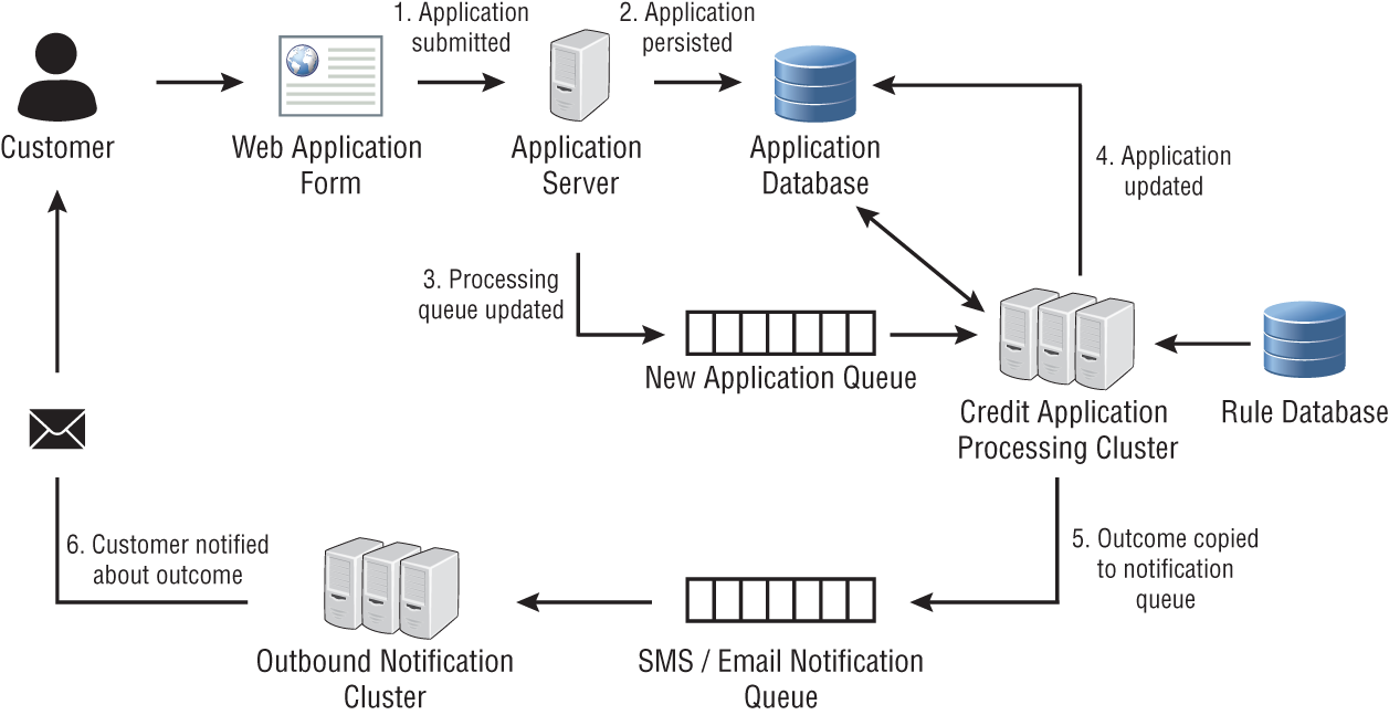
FIGURE 1.4 Architecture of a rule-based decision system
When an applicant submits a credit card application on the bank's website, a unique card application identifier is generated, and a row is added to a database by the web application. The web application also publishes a message onto a message queue; the content of the message contains the unique application identifier. A cluster of loan processing servers subscribe to the message queue and the first available servers will pick up the message and begin processing the credit card application. When the server reaches a decision, it will update the loan application in the database and publish a message on another message queue. The contents of this new message will contain all the information needed to send an SMS or email notification to the customer, informing the customer of the outcome.
How do you define the rules that will be used to make the decision? To start with you will need to create the rules based on your experience of the problem domain and qualities of the loan application form that you feel are favorable. If your business has another rule-based system that your solution is trying to replace, you may also be able to port some of the rules from the existing system.
Let's assume you do not have access to an existing system and need to define the business rules yourself. Looking at the fields in your loan application form, you decide that the following fields can be discarded from the decision-making process as you feel they are not likely to have any impact on the ability of individuals to keep up their monthly repayments:
- Name
- Sex
- Marital status
- Number of dependents in the household
- Homeowner status
You are now left with the following information that you can use to build your rules:
- Number of years lived at current address
- Number of addresses in the last 5 years
- Number of credit cards held with other banks
- Total amount of loan (excluding mortgage)
- Total income after tax
- Estimated regular monthly outgoings
- Total monthly repayments
You decide to create rules that will reject applications that meet any of the following criteria:
- Applicants that have lived less than 1 year at their current address.
- Applicants that have had more than three addresses in the last 5 years.
- Applicants that have two or more credit cards with other banks.
- Applicants whose disposable monthly income is less than 15% of their total income after tax.
These rules can be coded in any programming language using if-then-else statements. Figure 1.5 contains a flowchart that depicts the decision-making process using the rules you have defined.
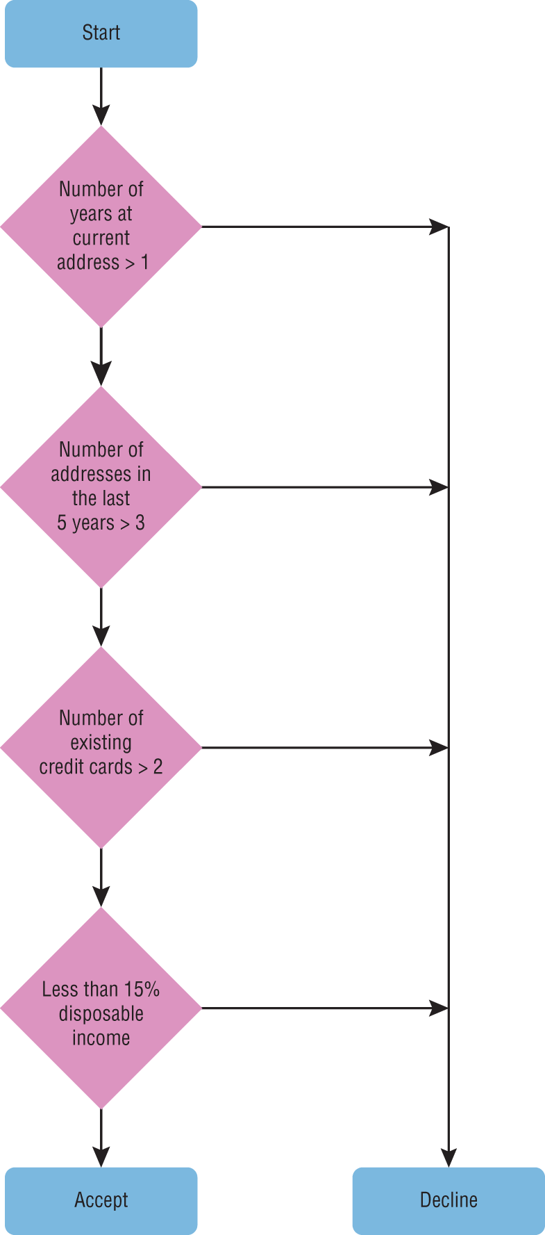
FIGURE 1.5 A flowchart depicting the decision-making process for a rule-based system
There is a possibility that the rules you have created and the initial assumptions you have made were not optimal, but you can always tailor the rules if you observe the losses due to missed payments exceed the bank's risk threshold. In time, as the volume of credit applications increases you will need to tailor your business rules to deal with the increased volume, and you are likely to encounter a few problems:
- Your rules become very complicated and interdependent; it becomes increasingly complex to replace old rules with new ones.
- Your rules have not been based on any numerical analysis; they have been created ad hoc to address increasing demand.
- Your rules do not account for changing patterns in the economy; for example, in the midst of a recession a larger number of people may end up missing their payments even though your rules predict that they should not. You will need to constantly keep updating your rules and that can be a costly and time-consuming process.
Let's now see how a machine learning–based system could be used to address these problems.
A Machine Learning–based System
Unlike a rule-based solution, you cannot create a machine learning solution without historical data from previous applicants. It is important to have data that is accurate and relevant to the problem you are trying to solve. You may be tempted to build your machine learning model using data from a different loan product, such as a personal loan. This is not recommended, as there could be trends in that data that are applicable only for personal loan applications.
You may be wondering why there was no need for historical data while building the rule-based system, and why defining the rules based on an intuitive understanding of the questions alone was sufficient. The reason is that in the rule-based approach, you were defining the rules based on your personal knowledge and experience of the problem domain. A machine-learning system, on the other hand, does not start with any prior knowledge of the problem domain. It does not have the intuitive capability of a human being. Instead, a machine learning system attempts to make its own inferences purely from the data it encounters. Not only do you need data, but also relevant data. If the data that is used to train the machine learning system is significantly different from what the system will encounter when asked to make predictions, the predictions are likely to be incorrect.
Just how much data will you need? There is no simple answer to that question. In general, machine learning algorithms require a lot of data to be trained effectively, but it is not just the quantity that matters; it is also the quality of the data. If your data has too many samples that follow a particular trend, then your machine learning system will be biased toward that trend.
For the purpose of this example, let's assume you have decided to pick the data for 5000 applicants randomly from your database, and exported these rows to a CSV file. These are all applicants that have applied for your credit card product and have either kept up with their regular payments or missed at most one payment. The input variables in this case would be answers to the questions asked on the form; the target variable will be a Boolean that indicates whether the applicant missed at most one payment.
Such type of data, where you already know the value of the target variable, is known as labeled data and is commonly used for training machine learning models. Not all data is labeled; in fact, the vast majority of data in the world is unlabeled. Using unlabeled (or partially labeled) data to train machine learning algorithms is an active area of research.
What if you want to build a machine learning solution, but have absolutely no data of your own, and can't wait months (or years) to collect high-quality labeled data? Your best option in this case would be to try to find existing datasets from free or paid sources on the Internet that are as close as possible to the problem domain you are working in. Chapter 2 provides links to several public machine learning datasets.
PICKING INPUT FEATURES
Once you have collected the labeled input data, you will need to perform basic statistical analysis on the data to pick input variables that are most likely to be relevant and prepare the input data for the machine learning model. Having the data in a CSV file makes it easy to load into data analysis tools. Most cloud-based data analysis tools allow you to upload CSV files, and some also support importing data from cloud-based relational databases.
Data visualization techniques are commonly used to get an indication of the spread and correlation of individual features. You will most likely build and train a model using an initial set of features and calculate the value of a performance metric while making predictions with the model. You will then retrain the model with additional input features and repeat as necessary as long as you observe a significant improvement in the value of the performance metric.
The number of features you choose will also impact the size of the training dataset you are likely to need. A model with 3 features could be built using a dataset of 500 items, whereas a model with 10 features will likely need a training dataset that consists of several thousands of items.
It may surprise you to learn that the bulk of a data scientist's job is looking at data and working out ways to use it. This work is often referred to as data munging, and involves several steps, including but not limited to:
- Finding out if there are any missing values in the data
- Working out the best way to handle missing values
- Examining the statistical distribution of the data
- Examining the correlation between input variables
- Creating new input variables by splitting or combining existing input variables
- NOTE Munge is a technical term coined by MIT students and means to transform data using a series of reversible steps to arrive at a different representation. Data munging is also known as data wrangling and feature engineering.
R, Python, Jupyter Notebook, NumPy, Pandas, and Matplotlib are commonly used for statistical analysis and feature engineering. Chapters 2 and 3 cover a number of techniques that can be used for feature engineering and data visualization to arrive at the final list of input features.
Let's now examine the questions on the application form and perform some simple feature engineering, based on your experience with the rule-based approach, to arrive at the inputs to our first machine learning model. Table 1.1 lists all the questions on the loan application form with their data types, range of expected values, and range of actual values as observed in 5000 samples.
TABLE 1.1: Type and Range of Data across 100 Sample Applications
| QUESTION | TYPE OF DATA | ACTUAL RANGE | MAXIMUM RANGE |
| Name | Free Text | Characters A–Z, some special characters | Characters A–Z, some special characters |
| Age | Continuous Numeric | 22–45 | 18–150 |
| Sex | Categorical | Male, Female, Undisclosed | Male, Female, Undisclosed |
| Number of years lived at current address | Continuous Numeric | 0–7 | 0–150 |
| Number of addresses in the last 5 years | Continuous Numeric | 1–6 | 1–10 |
| Number of credit cards held with other banks | Discrete Numeric | 1, 2, 3 | 1, 2, 3, 4, 5, 6, 7, 8, 9, 10 |
| Total amount of loan (excluding mortgage) | Continuous Numeric | 0–17500 | 0–10 million |
| Total income after tax | Continuous Numeric | 50000–200000 | 0–10 million |
| Estimated regular monthly outgoings | Continuous Numeric | 3000–15000 | 0–10 million |
| Total monthly repayments | Continuous Numeric | 0–1500 | 0–10 million |
| Homeowner status | Categorical | Yes or No | Yes or No |
| Marital status | Categorical | Single, Married, Undisclosed | Single, Married, Undisclosed |
| Number of dependents in the household | Discrete Numeric | 1, 2, 3 | 1, 2, 3, 4, 5, 6, 7, 8, 9, 10 |
It is quite clear that some of the answers are categorical while others are numeric. The numeric features themselves are either discrete or continuous and have different ranges of values.
Most machine learning models are designed to perform better on one type of feature over the other. Some statistical-based learning models are also sensitive to large numeric values. After examining the type of questions on the application form, the range of input values, and sample data for 5000 applicants, you decide that you want to use all of the answers on the application form as input features, except for the following:
- Name of the applicant
- Number of dependents
- Number of credit cards held with other banks
You also decide to engineer a new feature called Total Disposable Income, and split three categorical features into discrete numeric features as listed in Table 1.2.
TABLE 1.2: Transforming Categorical Features into Numeric Features
| ORIGINAL CATEGORICAL FEATURE | NEW NUMERIC FEATURE | ALLOWED VALUES/RANGE |
| Sex | SexIsMale | 0 or 1 |
| SexIsFemale | 0 or 1 | |
| SexIsUndisclosed | 0 or 1 | |
| Homeowner status | IsHomeOwner | 0 or 1 |
| IsNotHomeOwner | 0 or 1 | |
| Marital status | MaritalStatusIsSingle | 0 or 1 |
| MaritalStatusIsMarried | 0 or 1 | |
| MaritalStatusIsUndisclosed | 0 or 1 |
The new engineered feature Total Disposable Income is defined as:
Total Disposable Income = Total Income After Tax – Regular Monthly outgoings – Monthly Loan Repayments
Feature engineering techniques are covered in Chapter 2, but it is worth noting that some of the questions that have been answered as undisclosed are being treated as first-class values, as opposed to treating the question as missing an answer.
Table 1.3 lists the new set of input and engineered features, the expected range of values for each feature, and the actual range of values as observed in 5000 sample application forms.
TABLE 1.3: Modified Input Features
| FEATURE NAME | FEATURE DESCRIPTION | TYPE OF DATA | OBSERVED RANGE | MAXIMUM RANGE |
| F1 | Age | Continuous Numeric | 22–45 | 18–150 |
| F2 | SexIsMale | Discrete Numeric | 0, 1 | 0 or 1 |
| F3 | SexIsFemale | Discrete Numeric | 0, 1 | 0 or 1 |
| F4 | SexIsUndisclosed | Discrete Numeric | 0, 1 | 0 or 1 |
| F5 | Number of years lived at current address | Continuous Numeric | 0–7 | 0–150 |
| F6 | Number of addresses in the last 5 years | Continuous Numeric | 1–6 | 0–150 |
| F7 | Total Disposable Income | Continuous Numeric | 0–5000 | 0–10 million |
| F8 | Total amount of loan (excluding mortgage) | Continuous Numeric | 0–17500 | 0–10 million |
| F9 | Total income after tax | Continuous Numeric | 50000–200000 | 0–10 million |
| F10 | Estimated regular monthly outgoings | Continuous Numeric | 3000–15000 | 0–10 million |
| F11 | Total monthly repayments | Continuous Numeric | 0–1500 | 0–10 million |
| F12 | IsHomeOwner | Discrete Numeric | 0, 1 | 0 or 1 |
| F13 | IsNotHomeOwner | Discrete Numeric | 0, 1 | 0 or 1 |
| F14 | MaritalStatusIsSingle | Discrete Numeric | 0, 1 | 0 or 1 |
| F15 | MaritalStatusIsMarried | Discrete Numeric | 0, 1 | 0 or 1 |
| F16 | MaritalStatusIsUndisclosed | Discrete Numeric | 0, 1 | 0 or 1 |
It is quite clear that the range of allowed values for the features are not all the same. For example, F1 (Age) values lie in the range [18,100], whereas other feature values lie in the ranges [0,1], [0, 150], [1,10] and [0, 10000000]. Before you can use this data you will need to normalize the values of all the features to lie in the same range [0, 1]. Normalization is covered in Chapter 2, and involves transforming the value of each feature so that it lies in the interval [0, 1]. You will need to normalize both the training data as well as data on which your solution will make predictions.
You could also have chosen to transform the numeric features into categorical features by defining ranges of allowed values. For example, a given response to the total income after tax question, which is a continuous value between 0 and 10 million, could be converted into the following categorical value:
- Between0and100000
- Between100001and500000
- Above500001
There is no right or wrong way to engineer features. Sometimes the choice of machine learning algorithm dictates the type of features (numerical or categorical). Some algorithms, such as linear regression, work with numeric features; others that are based on decision trees work better with categorical features. Sometimes you start with a set of features only to realize that the predictive accuracy of the model trained on those features is not good enough and you need to start from scratch with new features, or perhaps a different algorithm or training technique.
PREPARING THE TRAINING AND TEST SET
Before you can build a machine learning model, you need to create separate training and testing datasets. The training set is used to build the model, whereas the test set is used to evaluate the performance of the model. The reason to have a separate training and test set is that a well-trained model will always perform well on the training set, as it has learned all the items in the training set. To truly measure the performance of the model, you need to present it data that it has not encountered during training.
Typically you will use 70% of the data for training and hold out 30% of the data for testing; however, other splits, such as 60:40, are also commonly used. When preparing the training and test set it is important to ensure that the members of the test set are well distributed, and do not exhibit bias toward any particular trend. For instance, if the training set consisted of a large proportion of applicants that were female and had annual incomes exceeding $100,000, the model is likely to incorporate this trend as part of its learning and perform poorly on other types of applicants. When a model performs well on the training set and poorly on the test set, the model is said to overfit the training data.
Cross-validation can help minimize the possibility of the model picking up on unexpected bias in the training set. The idea behind cross-validation is to shuffle the entire dataset randomly and divide it into a number of smaller sets (known as folds). If, for instance, the data were divided into 10 equal folds, the model would be trained and evaluated 10 times. During each training and evaluation cycle, one of the folds will be held out as the test set and the remaining nine will make the training set. This is illustrated in Figure 1.6.
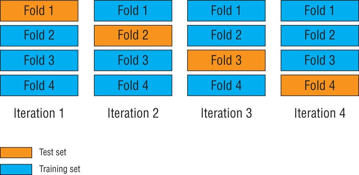
FIGURE 1.6 Cross-validation using multiple folds
Sometimes the bias is introduced during the data collection phase (also known as sampling bias), and no amount of cross-validation can help remove it. For instance, you may be building a model based on a dataset that contains information on consumer shopping trends collected during the Christmas holiday season. This data will be biased toward trends that are specific to holiday shopping, and a model built using this data will perform poorly if used to predict what consumers may buy over the course of the entire year. In such cases the best option is to collect more data to remove the sampling bias.
PICKING A MACHINE LEARNING ALGORITHM
There are a number of machine learning algorithms that can be used for classification tasks. In the current example, the objective is to decide, at the point of application, whether an applicant should be issued a credit card. The machine learning system that makes this decision is to be trained on data that is labeled to indicate if the customer has historically missed any payments (negative outcome), or if the customer did not miss a single payment (positive outcome).
The decision to issue the credit card is directly related to whether the machine learning system indicates the customer will default or not. This is a typical classification problem and a number of algorithms could be used:
- Logistic regression
- Decision trees
- Random forests
- XGBoost
- Neural networks
- Clustering-based techniques
The choice of algorithm is often influenced by factors such as desired accuracy, number of classes desired (binary vs. multi-class classification), availability of sufficient training data, time taken to train the model, memory footprint of the trained model, and resources required to deploy the model into production.
In this example we will make use of an algorithm called logistic regression, which is an algorithm that performs well for binary classification problems—problems that involve classifying something into one of two classes. Logistic regression builds upon the output of an algorithm called linear regression. Linear regression is a simple and effective algorithm for predicting continuous numeric values and assumes that the output variable can be expressed as a linear combination of the input features.
In effect, linear regression attempts to find the best line (or hyperplane in higher dimensions) that fits all the data points. The output of linear regression is a continuous, unbounded value. It can be a positive number or a negative number. It can have any value, depending on the inputs with which the model was trained.
In order to use a continuous value for binary classification, logistic regression converts it into a probability value between 0.0 and 1.0 by feeding the output of linear regression into a sigmoid function. The graph of the sigmoid function is presented in Figure 1.7. The output of the sigmoid function will never go below 0.0 or above 1.0, regardless of the value of the input.
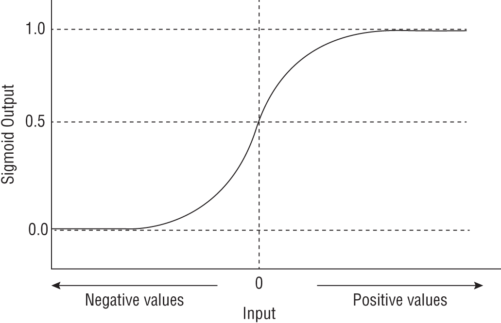
FIGURE 1.7 The sigmoid function
The output of the sigmoid function can be used for binary classification by setting a threshold value and treating all values below that as class A and everything above the threshold as class B (Figure 1.8).
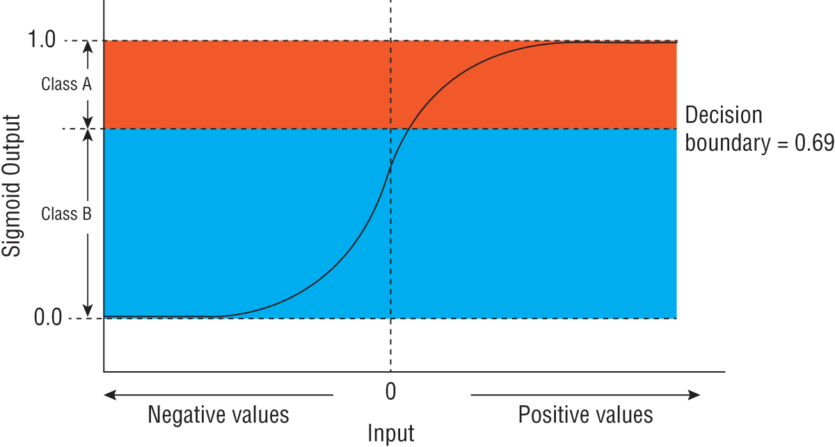
FIGURE 1.8 Using the sigmoid function for binary classification
While logistic regression is simple to understand, it may fail to provide good results if the relationship between the target variable and the input features is complex. In such a case you can consider using a tree-based model such as decision trees or an instance learning–based clustering model. You will learn more about model building in Chapter 4.
EVALUATING MODEL PERFORMANCE
Once you have built a model that can be used to determine if an applicant should be issued a credit card, you need to be able to quantitatively measure its performance. The purpose of evaluating a model is to determine how well it works on new data—models are evaluated using the labeled test set that was set aside during the training phase.
Since the model in this example attempts to solve a classification problem, you could simply count the number of times the model predicted the correct outcome and use this as an evaluation metric.
If issuing a credit card to an applicant is considered as the positive outcome, you can create a few additional metrics that go beyond simple counting:
- True positive count: The number of times the model predicted that a credit card should be issued to an applicant, and this decision matched the outcome in labeled test dataset.
- False positive count: The number of times the model predicted that a credit card should be issued to an applicant where the labeled test data indicated that applicant should not have been successful.
- True negative count: The number of times the model predicted that a credit card should not be issued to an applicant, and this decision matched the outcome in test dataset.
- False negative count: The number of times the model predicted that a credit card should not be issued to an applicant, and this decision was not correct according to the labeled test data.
You will learn to use these metrics and other performance evaluation and model tuning techniques in Chapter 5.
Summary
- Machine learning is a discipline within artificial intelligence that deals with creating algorithms that learn from data.
- Machine learning deals with the problem of creating computer programs that can generalize and predict information reliably and quickly.
- Machine learning is commonly used to implement fraud-detection systems, credit-scoring systems, authentication-decision engines, behavioral biometric systems, churn prediction, and product-recommendation engines.
- The type of training data that is required to train a machine learning system can be used to classify the machine learning system into supervised, unsupervised, or semi-supervised learning.
- Batch learning refers to the practice of training a machine learning model on the entire dataset before using the model to make predictions.
- Incremental learning, also known as online learning, refers to the practice of training a machine learning model continuously using small batches of data and incrementally improving the performance of the model.
- Instance-based learning systems make a prediction on new unseen data by picking the closest instance from instances in the training dataset.
- Model-based learning systems attempt to build a mathematical, hierarchical, or graph-based model that models the relationships between the inputs and the output.