In the previous chapter, we looked at the core strength of the Spark framework and the process to use it in different ways. This chapter focuses on how we can use PySpark to handle data. In essence, we would apply the same steps when dealing with a huge set of data points; but for demonstration purposes, we will consider a relatively small sample of data. As we know, data ingestion, cleaning, and processing are supercritical steps for any type of data pipeline before data can be used for Machine Learning or visualization purposes. Hence, we would go over some of the built-in functions of Spark to help us handle big data. This chapter is divided into two parts. In the first part, we go over the steps to read, understand, and explore data using PySpark. In the second part, we explore Koalas, which is another option to handle big data. For the entire chapter, we will make use of a Databricks notebook and sample dataset.
Load and Read Data
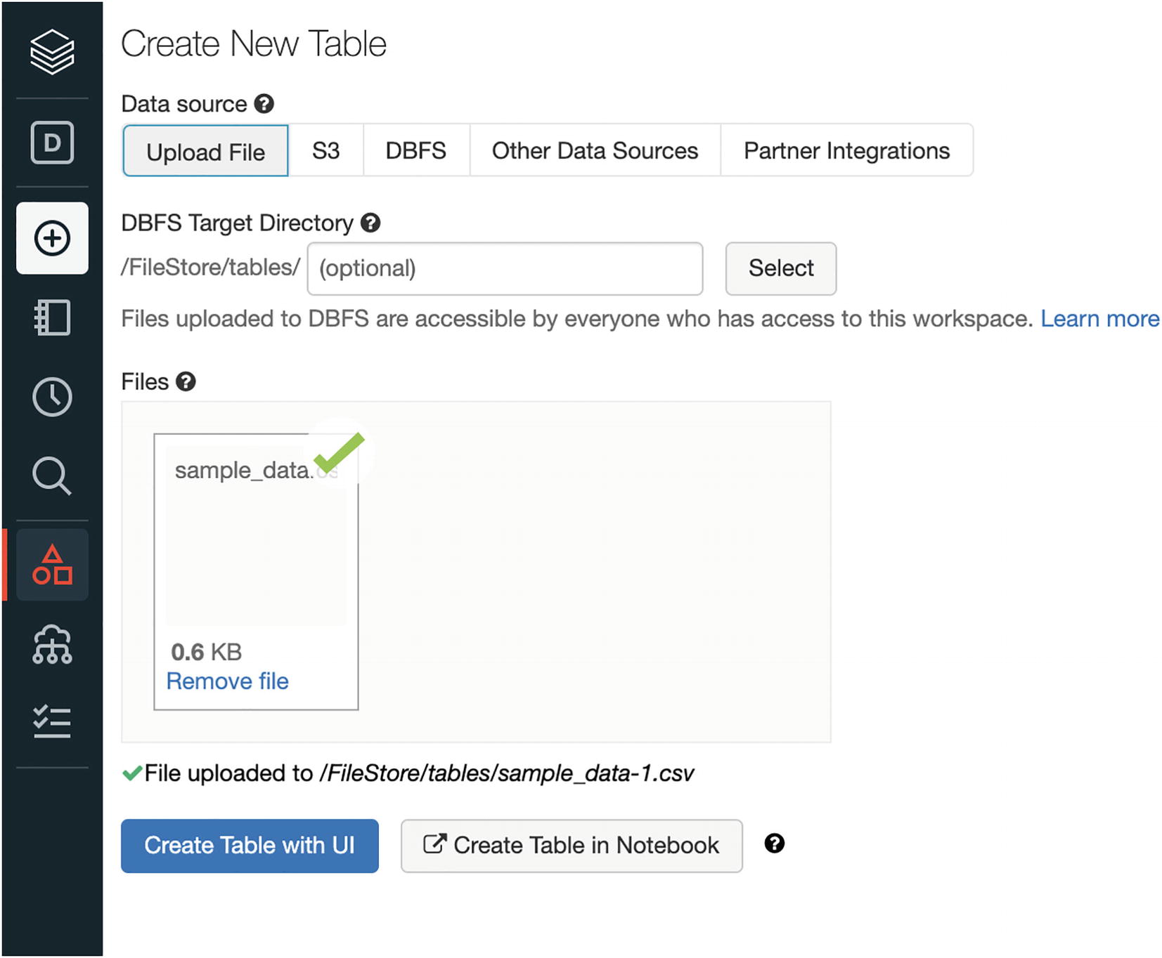
We need to ensure that the data file is uploaded successfully in the Databricks data layer. There are multiple data file types that could be uploaded in Databricks. In our case, we upload using the “Import & Explore Data” option as shown in Figure 2-1.
Figure 2-1
Upload data
We can upload the data file “sample_data.csv” in order to read it in the Databricks notebook. The default file location would be mentioned at the bottom as shown in Figure 2-2.
Figure 2-2
Access data
The next step is to spin up a cluster and attach a new Databricks notebook to it. We can go to the Compute option and start a new cluster. For those who might be not familiar with a cluster, it’s a group of machines on a cloud platform such as AWS or Google Cloud Platform. The size of the cluster depends on the tasks and amount of data one is dealing with. There are clusters with hundreds of machines, but in our case, we would be leveraging the default cluster provided by Databricks.
Once the cluster is active, we can create a new notebook. The first set of commands are to import PySpark and instantiate SparkSession in order to use PySpark:
We can update the read format argument in accordance with the file format (.csv, JSON, .parquet, table, text). For a tab-separated file, we need to pass an additional argument while reading the file to specify the delimiter (sep=' '). Setting the argument inferSchema to true indicates that Spark in the background will infer the datatypes of the values in the dataset on its own:
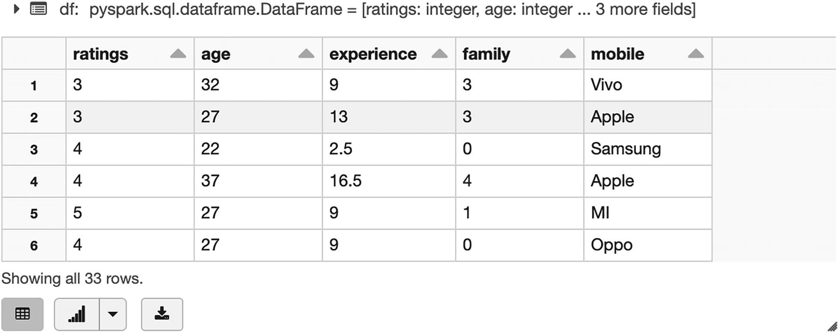
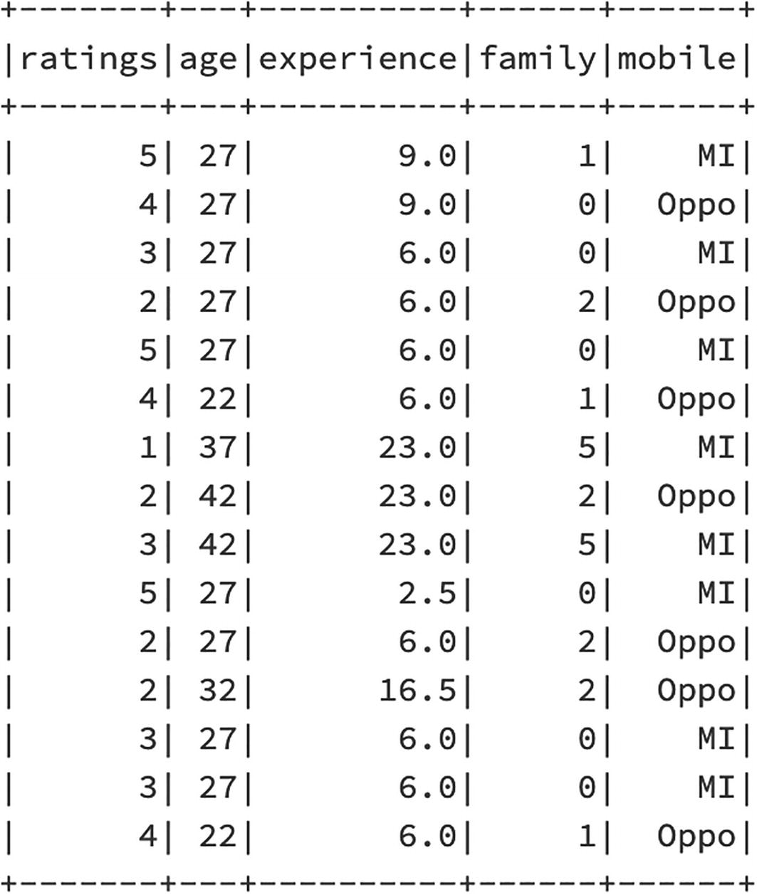
The preceding command creates a Spark dataframe with the values from our sample data file. We can consider this as an Excel spreadsheet in tabular format with columns and headers. We can now perform multiple operations on this Spark dataframe. We can use the display function to look at the dataset:
[In]: display(df)
We can also make use of the show function, which displays the data fields from the top row. Pandas users heavily make use of functions such as head and tail to sneak a peek into the data. Well, those are applicable here as well, but the output might look a bit different compared with display or show as it prints it in forms of rows. We can also pass the number of rows to be displayed by passing the value of n as an argument to show/head/tail:
[In]: df.show(5)
[In]: df.head(5)
[In]: df.tail(3)
We can print the list of column names that are present in the Dataframe using the “columns” method. As we can see, we have five columns in the Dataframe. We can observe the datatype for each of the columns using dtypes. Finally, one of the easiest ways to understand the Dataframe is to use printSchema, which provides a list of columns along with their datatypes:
[In]: df.columns
[In]: df.dtypes
[In]: df.printSchema()
We can use the count method to get the total number of records in the Dataframe. We can also use describe to understand statistical measures of different numerical columns in the Dataframe. For numerical columns, it returns the measure of center and spread along with the count. For non-numerical columns, it shows the count and the min and max values, which are based on an alphabetic order of those fields and doesn’t signify any real meaning. We could also pass specific column names in order to view the details of only selected data fields:
[In]: df.count()
[In]: len(df.columns)
[In]: df.describe().show()
[In]: df.describe('age').show()
Moving on to the next data processing step – filtering data. It is a very common requirement to filter records based on conditions. This helps in cleaning the data and keeping only relevant records for further analysis and building robust Machine Learning models. Data filtering in PySpark is pretty straightforward and can be done using two approaches:
1.
filter
2.
where
Data Filtering Using filter
Data filtering could be based on either a single column or multiple columns. The filter function in PySpark helps us to refine data based on specified conditions. If we were to filter data where the value of column “age” is less than 30, we could simply apply the filter function:
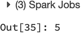
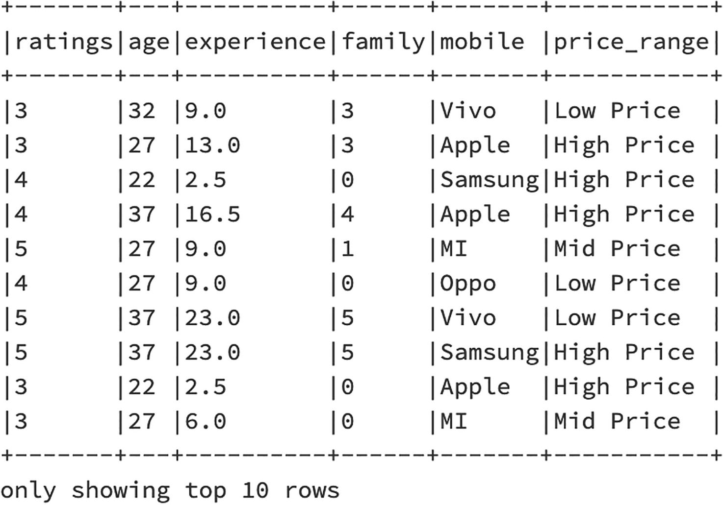
[In]: df.filter(df['age']<30).show()
[Out]:
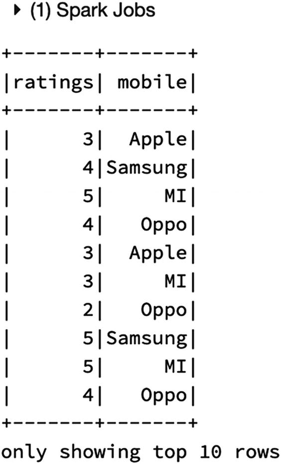
As we can observe, we have all data columns as part of the filtered output for which the age column has values of less than 30. We can apply further filtering using “select” to print only specific columns. For example, if we want to view the ratings and mobile for customers whose age is less than 30, we can do that by using the select function after applying filter to the age column:
If data filtering is based on multiple columns, then we can do it in a couple of ways. We can either use sequential filtering in PySpark or make use of (&,|) operators to provide multiple filter conditions. Let us say we want customers with age less than 30 and who are only “Oppo” users. We apply filter conditions in sequence:
We can also use operators like & and | to apply multiple filter conditions and get the required data. In the following example, we filter for Oppo mobile users who have experience of greater than or equal to 9 using “&”. In the follow-up example, we make use of the “or” condition to filter records with either “Oppo” users or “MI” users:
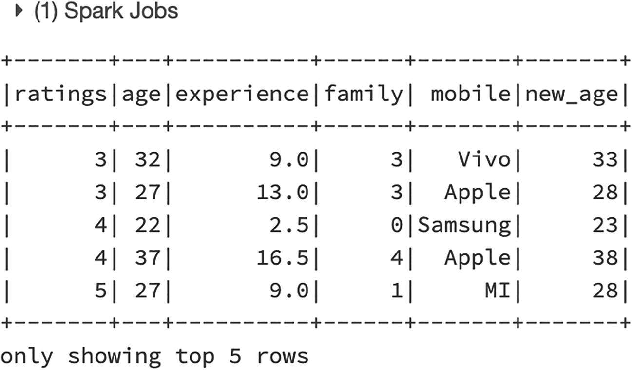
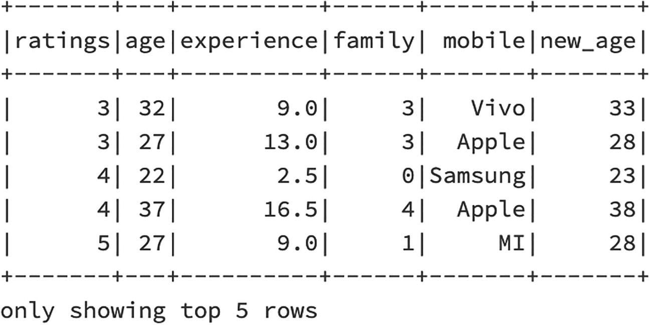
We can add a new column in the Spark dataframe using the withColumn function in PySpark. For example, if we were to create a new column (new age) in the Dataframe by using the age column, we would simply use the withColumn function and add one year to the age column. This would result in a new column being created with updated values. This doesn’t actually transform the Dataframe until it’s assigned to the old Dataframe or a new Dataframe. So if we were to print our Dataframe again, we would observe that the new age column is missing as it wasn’t assigned to the df Dataframe while creating it:
In terms of aggregating data with respect to individual columns, we can use the groupBy function in PySpark and cut the data based on various measures. For example, if we were to look at the number of users for every mobile brand, we would run a groupBy on “mobile” and take a count of users:
[In]: df.groupBy('mobile').count().show()
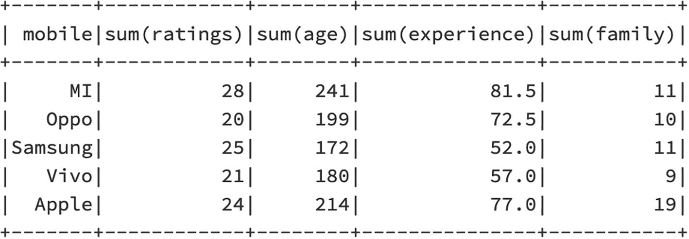
The aggregate measure can be changed based on the requirement such as count, sum, mean, or min. In the following example, we run an aggregate sum of values in other columns for every mobile brand:
[In]: df.groupBy('mobile').sum().show()
If we need different aggregate measures for specific columns, then we can make use of agg along with groupBy as shown in the following example:
In order to find the distinct values in a Dataframe column, we can use the distinct function along with count as shown in the following:
[In]: df.select('mobile').distinct().count()
In this part, we will understand UDFs – user-defined functions. Many times, we have to apply certain conditions and create a new column based on values in other columns of the Dataframe. In Pandas, we typically use the map or apply function to replicate such requirement. In PySpark, we can use UDFs to help us transform values in the Dataframe.
There are two types of UDFs available in PySpark:
1.
Conventional UDF
2.
Pandas UDF
Pandas UDFs are much more powerful in terms of execution speed and processing time. We will see how to use both types of UDFs in PySpark.
First, we need to import udf from PySpark and define the function that we need to apply to an existing Dataframe column. Now we can apply a basic UDF either by using a lambda or typical Python function. In this example, we define a custom Python function price range that returns if the mobile belongs to the High Price, Mid-Price, or Low Price category based on the brand. The next step is to declare the UDF and its return type (StringType in this example). Finally, we can use withColumn and mention the name of the new column to be formed along with applying the UDF and passing the relevant Dataframe column (mobile):
As we can observe, a new column gets added to the DataFrame containing return values from the UDF being applied on original mobile column.
Pandas UDF
As mentioned before, Pandas UDFs are way faster and efficient compared with their peers. There are two types of Pandas UDFs:
1.
Scalar
2.
GroupedMap
Using a Pandas UDF is quite similar to using a basic UDF. We have to first import pandas_udf from pyspark.sql.functions and apply it on any particular column to be transformed:
[In]: from pyspark.sql.functions import pandas_udf
In this example, we define a Python function that calculates the number of years left in a user’s life assuming life expectancy of total 100 years. It is a very simple calculation. We subtract the current age of the user from 100 using the Python function:
[In]:
def remaining_yrs(age):
yrs_left=(100-age)
return yrs_left
Once we create the pandas UDF (length_udf) using the Python function (remaining_yrs), we can apply it on the age column and create a new column yrs_left:
The preceding example showed how to use a Pandas UDF on a single dataframe column, but sometimes we might need to use more than one column. Hence, let’s go over one more example where we understand the method of applying a Pandas UDF on multiple columns of a dataframe. Here we will create a new column, which is simply the product of ratings and experience columns. As usual, we define a Python function and calculate the product of the two columns:
[In]:
def prod(rating,exp):
x=rating*exp
return x
[In]: prod_udf = pandas_udf(prod, DoubleType())
After creating the Pandas UDF, we can apply it on both of the columns (ratings, experience) to form the new column (product):
We can use the dropDuplicates function in order to remove the duplicate records from the Dataframe. The total number of records in this Dataframe is 33, but it also contains 7 duplicate records, which can easily be confirmed by dropping those duplicate records as we are left with only 26 rows:
[In]: df.count()
[Out]: 33
[In]: df=df.dropDuplicates()
[In]: df.count()
[Out]: 26
In order to delete a column or multiple columns, we can use the drop functionality in PySpark:
[In]: df.drop('age').show()
[In]: df.drop('age','experience').show(5)
[Out]:
Writing Data
Once we have the processing steps completed, we can write the clean Dataframe to a desired location (local/cloud) in the required format. In our case, we simply write back the sample processed data to Databricks FileStore. We can choose the desired format (.csv, .parquet, etc.) to save the final Dataframe.
CSV
If we want to save it back in the original .csv format as a single file, we can also use the coalesce function in Spark:
If the dataset is huge and involves a lot of columns, we can choose to compress it and convert it into a .parquet file format. It reduces the overall size of the data and optimizes the performance while processing data because it works on a subset of required columns instead of the entire data. We can convert and save the Dataframe into the .parquet format easily by mentioning the format as parquet as shown in the following:
Data scientists and data engineers often start their data wrangling journey with Pandas as it is the most established data processing library out there along with NumPy and scikit-learn for Machine Learning. Given the adoption rate of Pandas is so high, there is no debate around the use of Pandas as a standard data processing library. It is quite mature in terms of offerings, simple APIs, and extensibility. However, one of the key limitations of using Pandas is that you can hit a roadblock if the data you’re dealing with is very big in terms of size as Pandas is not very scalable. The core reason is Pandas is meant to run on a single-worker machine instead of a multiple-worker setup. Hence, for large datasets, Pandas will either run incredibly slow or usually throw memory errors. However, for proof of concepts (POCs) and minimum viable products (MVPs), Pandas is still the go-to library. The other libraries such as Dask try to address the scalability issue that Pandas has by processing data in partitions and speeding up things in the execution front.
There are some challenges that still persist. Hence, when it comes to handling big data and distributed processing frameworks, Spark becomes the de facto choice for the data community out there. One of the new offerings by Databricks is the open source library called Koalas. It provides a Pandas DataFrame API on top of Apache Spark. As a result, it takes advantage of the Spark implementation of DataFrames, query optimization, and data source connectors all with Pandas syntax. In essence, it offers a nice alternative to use the power of Spark even while working with Pandas.
Note
This Koalas library is still under active development and covering more than 75% of the Pandas API.
There are a number of benefits of using Koalas over Pandas when dealing with large datasets as it allows to use similar syntax as that of Pandas without worrying too much about the underlying Spark details. One can easily transition between Pandas and Koalas Dataframes and into Spark Dataframes. It also offers easy integration with SQL through which one can run multiple queries on a Koalas Dataframe.
The first step is to import koalas and convert a Spark Dataframe to a Koalas Dataframe:
[In]: from databricks import koalas as ks
[In]: k_df = df.to_koalas()
If we look at the type of the new Dataframe, it would return it as a Koalas Dataframe type:
[In]: type(k_df)
[Out]: databricks.koalas.frame.DataFrame
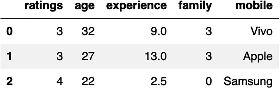
Now we can simply start using the Pandas functions and syntax to transform and process the dataset. For example, a simple df.head(3) would return the top three rows of the dataframe:
[In]: k_df.head(3)
We can also look at the shape of the dataframe now using the shape function, which isn’t possible in PySpark directly:
[In]: k_df.shape
Finally just to reinforce, we can also use groupby, instead of groupBy, on a Koalas Dataframe to aggregate values based on different columns:
[In]: k_df.groupby(['mobile']).sum()
Conclusion
In this chapter, we looked at the steps to read, explore, process, and write data using PySpark. We also looked at Koalas, which offers Pandas users to process data using Spark under the hood.