This is the last chapter of the book and focuses on the techniques to tackle text data using PySpark. Today text-form data is being generated at a lightning pace with multiple social media platforms offering users the options to share their reviews, suggestions, comments, etc. The area that focuses on making machines learn and understand textual data to perform some useful tasks is known as Natural Language Processing. Text data could be structured or unstructured, and we must apply multiple steps to make it analysis ready. The NLP field is already a huge area of research and has an immense number of applications being developed that use text data such as chatbots, speech recognition, language translation, recommender systems, spam detection, and sentiment analysis. This chapter demonstrates a series of steps to process text data and apply Machine Learning algorithms on it. It also showcases sequence embeddings that are learned using word2vec in PySpark as a bonus part.
Steps Involved in NLP
Text data can be very messy sometimes, and it needs careful attention to bring it to a stage where it can be used in the right way. There are multiple ways in which text data can be cleaned and refined. For example, regular expressions are very powerful when it comes to filtering, cleaning, and standardizing text data. However, regular expressions are not the focus area in this chapter. Rather, we look at the steps to prepare text data in a form where we can fit a ML model on it. The five major steps involved in handling text data for ML modeling are
1.
Reading the corpus
2.
Tokenization
3.
Cleaning/stopword removal
4.
Stemming
5.
Converting into numerical form
Before jumping into the steps to load and clean text data, let’s get familiar with a term known as corpus as this would keep appearing in the rest of the chapter.
Corpus
A corpus is known as an entire collection of text documents, for example, a collection of emails, messages, or user reviews. This group of individual text items is known as a corpus. The next step in text processing is tokenization
Tokenize
The method of dividing the given text sequence/sentence or collection of words of a text document into individual words is known as tokenization. It removes the unnecessary characters such as punctuations. The final units post-tokenization are known as tokens. Let’s say we have the following text:
Input: He really liked the London City. He is there for two more days.
Tokenization would result in the following tokens. We end up with 13 tokens for the input text:
He, really, liked, the, London, City, He, is, there, for, two, more, days
Let us see how we can do tokenization using PySpark. The first step is to create a SparkSession object to use Spark. We take some sample user IDs and reviews to create a text Dataframe as shown in the following:
[In]: df=spark.createDataFrame([(1,'I really liked this movie'),
(2,'I would recommend this movie to my friends'),
(3,'movie was alright but acting was horrible'),
(4,'I am never watching that movie ever again')],
['user_id','review'])
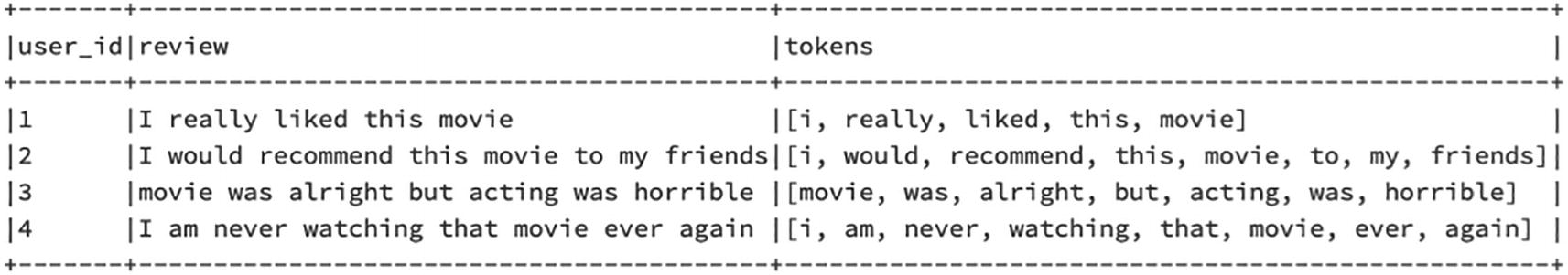
[In]: df.show(4,False)
[Out]:
In this Dataframe, we have four sentences for tokenization. The next step is to import Tokenizer from the Spark library. We must then pass the input column and name the output column after tokenization. We use the transform function to apply tokenization to the review column:
We get a new column named tokens, which contains the tokens for each sentence.
Stopword Removal
As you can observe, the tokens column contains very common words such as “this,” “the,” “to,” “was,” “that,” etc. These words are known as stopwords, and they seem to add very little value to the analysis. If they are to be used in analysis, it increases the computation overheads without adding too much signal. Hence, it’s preferred to drop these stopwords from the tokens. In PySpark, we use StopWordsRemover to remove the stopwords:
As you can observe, the stopwords like “I,” “this,” “was,” “am,” “but,” and “that” are removed from the tokens column.
Bag of Words
Now that we have the key tokens created from the text data, we now need a mechanism to convert the tokens into a numerical form because we know for a fact that a Machine Learning algorithm works on numerical data. Text data is generally unstructured and varies in its length. Bag of words allows to convert the text data into numerical vector form by considering the occurrence of the words in text documents, for example:
Doc 1: The best thing in life is to travel
Doc 2: Travel is the best medicine
Doc 3: One should travel more often
The list of unique words appearing in all the documents is known as vocabulary. In the preceding example, we have a total of 13 unique words appearing that are part of the vocab. Any of these three documents can be represented by this vector of fixed size 13 using a Boolean value (1 or 0):
The
Best
thing
in
life
is
to
travel
medicine
one
should
more
often
Doc 1:
The
Best
thing
in
life
is
to
travel
medicine
one
should
more
often
1
1
1
1
1
1
1
1
0
0
0
0
0
Doc 2:
The
Best
thing
in
life
is
to
travel
medicine
one
should
more
often
1
1
0
0
0
1
0
1
1
0
0
0
0
Doc 3:
The
Best
thing
in
life
is
to
travel
medicine
one
should
more
often
0
0
0
0
0
0
0
1
0
1
1
1
1
Bag of words does not consider the order of words in the document and the semantic meaning of the word and hence is the most baseline method to represent the text data in numerical form. There are other ways by which we can convert the textual data into numerical form, which are covered in the following section. We will use PySpark to go through each one of these methods.
CountVectorizer
In bag of words, we saw the representation of the occurrence of a word by simply 1 or 0 and did not consider the frequency of the word. The count vectorizer instead takes the total count of the tokens appearing in the document. We will use the same text documents that we created earlier during tokenization. We first import CountVectorizer:
[In]: from pyspark.ml.feature import CountVectorizer
As we can observe, each row is represented as a dense vector. It shows that the vector length is 11 and the first sentence contains three values at the 0th, 4th, and 9th indexes.
To validate the vocabulary of the count vectorizer, we can simply use the vocabulary function:
[In]: count_vec.fit(refined_df).vocabulary
[Out]:
Hence, the vocabulary size for the preceding sentences is 11; and if you look at the features carefully, they are like the input feature vector that we have been using for Machine Learning in PySpark. The drawback of using the CountVectorizer method is that it doesn’t consider the co-occurrences of words in other documents. In simple terms, the words appearing often would have larger impact on the feature vector. Hence, another approach to convert text data into numerical form is TF-IDF (Term Frequency – Inverse Document Frequency).
TF-IDF
This method tries to normalize the frequency of token occurrence based on other documents. The whole idea is to give more weight to the token if appearing high number of times in the same document but penalize if it is appearing higher number of times in other documents as well. This indicates that the token is common across the corpus and is not as important as its frequency in the current document indicates.
Term Frequency: Score based on the frequency of the word in the current document
Inverse Document Frequency: Score based on the number of documents that contain the current word
Now, we create features based on TF-IDF in PySpark using the same refined df Dataframe:
[In]: from pyspark.ml.feature import HashingTF,IDF
Now that we understand the steps involved in dealing with text processing and feature vectorization, we can build a text classification model and use it for predictions on text data. The dataset that we are going to use is a sample of the open source movie lens reviews data, and we’re going to predict the sentiment of the given review (positive or negative). Let’s start with reading the text data first and creating a Spark Dataframe:
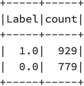
Some of the records got filtered out, and we are now left with 6990 records for the analysis. The next step is to validate the number of reviews for each class:
[In]: text_df.groupBy('Sentiment').count().show()
[Out]:
+---------+-----+
|Sentiment|count|
+---------+-----+
| 0| 3081|
| 1| 3909|
+---------+-----+
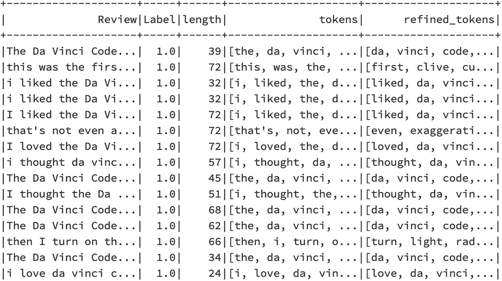
We are dealing with a balanced dataset here as both classes have an almost similar number of reviews. Let us look at a few of the records in the dataset. As a next step, we create a new integer-type Label column and drop the original Sentiment column, which was string type:
There is no major difference between the average length of the positive review and that of the negative review. The next step is to start the tokenization process and remove stopwords:
Since we’re now dealing with tokens only instead of an entire review, it would make more sense to capture the number of tokens in each review rather than using the length of the review. We create another column (token count) that gives the number of tokens in each row:
Now that we have the refined tokens after stopword removal, we can use any of the preceding approaches to convert text into numerical features. In this case, we use CountVectorizer for feature vectorization for the Machine Learning model:
Please evaluate the performance of the logistic regression model using accuracy metrics on test data.
Sequence Embeddings
Let us move on to the second part of this chapter that covers sequence embeddings. We looked at different ways to convert text into numerical form using bag of words, count vectorizer, TF-IDF, etc. However, none of these considers the semantics, context, or order in which the text or neighboring text appears. However, we know for a fact that context and sequence matter a lot for understanding any text data. That’s where embeddings can shine and provide a robust mechanism to understand and represent text data in a numerical form, which is more effective compared with other approaches.
Let us take an example to understand sequence embeddings better. We all use mobile phones connected to the Internet all the time. We use so many apps throughout the day like Facebook, Amazon, Twitter, etc. Some of these apps provide relevant content or items to us to keep us engaged, whereas sometimes we struggle finding the right information or product. Similarly, millions of people use the same apps every day, yet each one of them takes a different route/set of steps to seek the relevant information/product. This could be termed as individual user journey. Many times, people are left frustrated with the app experience or disappointed due to missing information. In such cases, it becomes difficult to find out if the user was satisfied with the overall experience. The individual user journeys vary from the rest on multiple parameters such as total time spent, total number of pages viewed, liked content/product, or reviewed content/product.
So, if a business were to understand their customers better, they would need to understand which set of user journeys are resulting into less conversion or drop-off vs. which user journeys are more engaging and successful.
Sequence embedding is a powerful way that offers us the flexibility to not only compare any two individual user journeys but also use them to predict the probability of a visitor’s conversion.
Embeddings
As mentioned already, the techniques like count vectorizer, TF-IDF, and hashing vectorization do not consider semantic meanings of the text or the context in which words are present. Embeddings are unique in terms of capturing the context of the words and representing it in such a way that words with similar meanings are represented with a similar sort of embeddings. There are two ways to calculate the embeddings:
1.
Skip gram
2.
Continuous bag of words (CBOW)
Now we would not be going in depth to cover these techniques mentioned, but on a high level, both the methods give the embedding values that are the weights of the hidden layer in a neural network. The embedding vector size can be chosen based on a requirement, but a size of 100 works well for most of the cases. We will make use of word2vec in Spark to create embeddings. We will use a sample retail dataset for this exercise:
As we can see, the dataset contains six columns. It includes the unique user ID, the web page category being viewed, visit number, time spent on the page category, and conversion status. The total number of records in the dataset is close to 1M, and there are 0.1M unique users. All the columns are of the string datatype:
The whole idea of sequence embeddings is to translate the series of steps taken by the user during their online journey into a page sequence that can be used for calculating embedding scores. The first step is to remove any of the consecutive duplicate pages during the journey of a user. We create an additional column that captures the previous page of the user using the window function in PySpark:
[In]: w = Window.partitionBy("user_id").orderBy('timestamp')
Now, we create a function to check if the current page is like the previous page and indicate the same in a new column indicator. indicator_cumulative is the column to track the number of distinct pages during the user journey:
In the next stage, we calculate the aggregated time spent on similar pages so that only a single record can be kept for representing consecutive pages:
Finally, we use collect list to combine all the pages of the user journey into a single list and for time spent as well. As a result, we end with a user journey in the form of a page list and time spent list:
We can now move to create embeddings using the word2vec model by feeding it the user journey sequence. The embedding size is kept to 100 for this part:
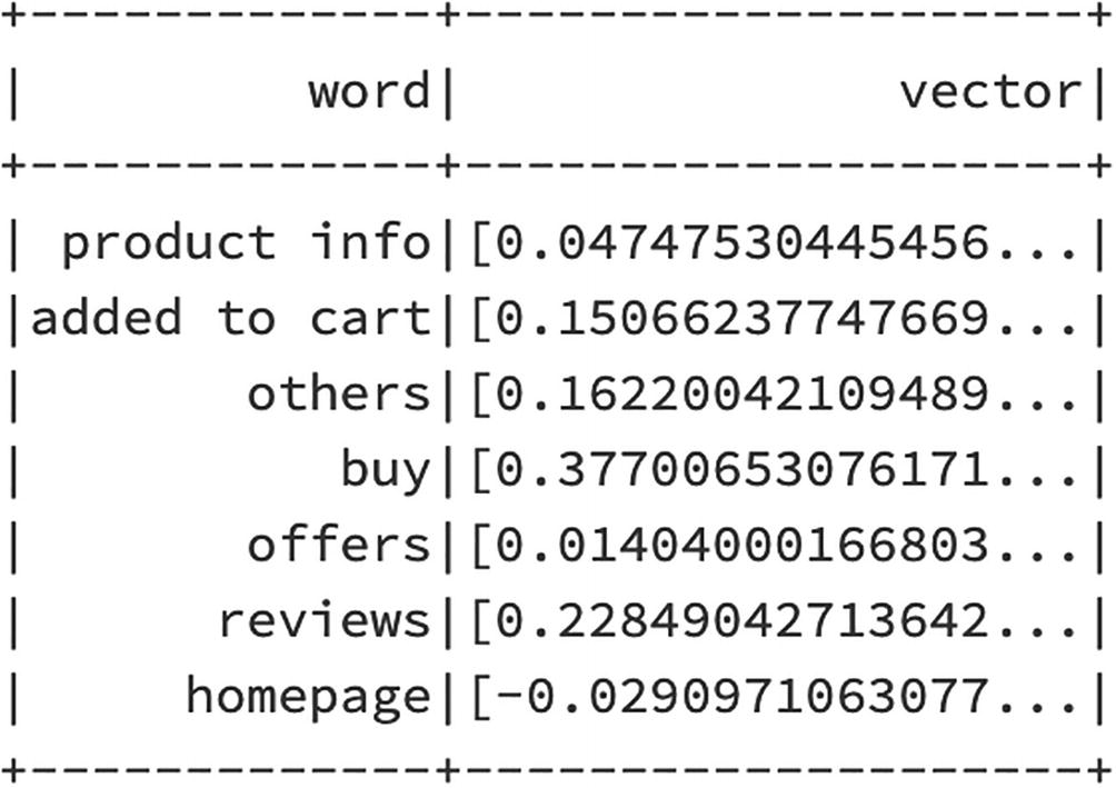
We can extract embeddings for each page category using getVectors(), but do ensure to change the datatype of the embeddings to double as the embeddings’ original format is vector in Spark:
As we can observe, the vocabulary size is 7 because we were dealing with seven page categories only. Each of these page categories now can be represented with the help of the embedding vector of size 100:
[In]: unique_pages = [i.word for i in page_categories]
[In]: print(unique_pages)
[Out]:
In order to visualize the embeddings of each of the page categories, we can convert the embeddings Dataframe to a Pandas Dataframe and later use matplotlib to plot the embeddings:
In order to better understand the relation between these page categories, we can use the dimensionality reduction technique (PCA) and plot these seven page embeddings on a two-dimensional space:
[In]: from sklearn.decomposition import PCA
[In]: pca = PCA(n_components=2)
[In]: pca_df = pca.fit_transform(X)
[In]: pca_df
[Out]:
[In]: import matplotlib.pyplot as plt
[In]: %matplotlib inline
[In]: plt.figure(figsize=(10,10))
[In]: plt.scatter(pca_df[:, 0], pca_df[:, 1])
[In]: for i,unique_page in enumerate(unique_pages):
As we can clearly observe, the embeddings of product info and homepage are near to each other in terms of similarity. Offers and reviews are very far when it comes to representation through embeddings. These individual embeddings can be combined and used for user journey comparison and classification using Machine Learning.
Conclusion
In this chapter, we covered the steps to do text processing using PySpark and creating sequence embeddings for representing online user journey data.
Overall in the book, we looked at multiple sets of algorithms to solve different problems right from linear regression to building a recommender system in PySpark. Again, we used some standard datasets (small and mid-size), but the same codebase could be applied on big datasets as well without changing too many things. Spark provides the flexibility to create customized pipelines as per requirement of the workflow. Now sometimes Spark might be an overkill to solve a small problem or for a small POC (proof of concept) because Pandas and sklearn could handle that much data. Hence, one should carefully evaluate the resource and tool landscape before starting to write code. There could be a bunch of metrics on which the right framework could be chosen such as size of data, scale of the project, timelines, latency rate, resources available, costs, etc. The bottom line is that one can leverage the power of Spark to deal with large data and build scalable ML models very quickly.