In brick-and-mortar stores, we have salespeople guiding and recommending us the relevant products while shopping. On the other hand, on online retail platforms, there are zillions of different products available, and we have to navigate ourselves to find the right product. The situation is that users have too many options and choices available, yet don’t like to invest a lot of time going through the entire catalogue of items. Hence, the role of recommender systems (RSs) becomes critical for recommending relevant items and driving customer conversion.
Traditional physical stores use a planogram to arrange the items in such a way that can increase the visibility of high-selling items and can increase revenue, whereas online retail stores need to keep it dynamic based on the preference of each individual customer rather than keeping it the same for everyone.
Recommender systems are mainly used for auto-suggesting the right content or product to the right user in a personalized manner to enhance the overall experience. Recommender systems are really powerful in terms of using huge amount of data and learning to understand the preference for specific users. Recommendations help users to easily navigate through millions of products or tons of content (articles/videos/movies) and show them the right item/information that they might like or buy. So, in simple terms, a RS helps discover information on behalf of the users. Now, it depends on the users to decide if the RS did a good job at recommendations or not, and they can choose to either select the product/content or discard and move on. Each of the decisions of users (positive or negative) helps to retrain the RS on latest data to be able to give even better recommendations. In this chapter, we will go over how the RS works and what are different types of techniques used under the hood for making these recommendations. We will also build a recommender system using PySpark.
Recommendations
Recommender systems can be used for multiple purposes in the sense of recommending various things to the users. For example, some of them might fall in the following categories:
1.
Retail products
2.
Jobs
3.
Connections/friends
4.
Movies/music/videos/books/articles
5.
Ads
The “What to Recommend” part totally depends on the context in which the RS is used and can help the business to increase revenues by providing most likely items that users can buy or increasing the engagement by showcasing relevant content at the right time. The RS takes care of the critical aspect that the product or content that is being recommended should be something that users might like but would not have discovered on their own. Along with that, the RS also needs an element of varied recommendations to keep it interesting enough. Examples of heavy usage of RSs by businesses today are Amazon products, Facebook’s friend suggestions, LinkedIn’s “People You May Know,” Netflix’s movies, YouTube’s videos, Spotify’s music, and Coursera’s courses.
The impact of these recommendations is proving to be immense from a business standpoint, and hence more time is being spent in making these RSs more efficient and relevant. Some of the immediate benefits that RSs offer in retail settings are
1.
Increased revenue
2.
Positive reviews and ratings by users
3.
Increased engagement
For the other verticals such as ad recommendations and other content recommendations, the RS helps immensely to help them find the right thing for users and hence increase adoptions and subscriptions. Without the RS, recommending online content to millions of users in a personalized manner or offering generic content to each user can be incredibly off target and lead to negative impact on users.
Now that we know the usage and features of RSs, we can take a look at different types of RSs. There are mainly five types of RSs that can be built:
1.
Popularity-based RS
2.
Content-based RS
3.
Collaborative filtering (CF)–based RS
4.
Hybrid RS
5.
Association rule mining–based RS
We will briefly go over each one of these except for the last item, that is, association rule mining–based RS, as it’s out of scope for this book.
Popularity-Based RS
This is the most basic and simplest RS that can be used to recommend products or content to the users. It recommends items/content based on items/content bought/viewed/liked/downloaded by most of the users. While it is easy and simple to implement, it doesn’t produce relevant results as the recommendations stay the same for every user, but it sometimes outperforms some of the more sophisticated RSs. The way this RS is implemented is by simply ranking the items on various parameters and recommending the top-ranked items in the list. As already mentioned, items or content can be ranked by
1.
No. of times downloaded
2.
No. of times bought
3.
No. of times viewed
4.
Highest rated
5.
No. of times shared
6.
No. of times liked
This kind of RS directly recommends the best-selling or most watched/bought items to the customers and hence increases the chances of customer conversion. The limitation of this RS is that it is not hyper-personalized.
Content-Based RS
This type of RS recommends similar items to the user that the user has liked in the past. So the whole idea is to calculate a similarity score between any two items and recommend to the user based upon the profile of the user’s interests. We start with creating item profiles for each of the items. Now these item profiles can be created in multiple ways, but the most common approach is to include information regarding the details or attributes of the item. For example, the item profile of a movie can have values on various attributes such as Horror, Art, Comedy, Action, Drama, and Commercial, as shown in the following:
Movie ID
Horror
Art
Comedy
Action
Drama
Commercial
2310
0.01
0.3
0.8
0.0
0.5
0.9
The preceding table is an example of an item profile, and each of the items would have a similar vector representing its attributes. Now, let’s assume the user has watched ten such movies and really liked them. So, for that particular user, we end with an item matrix as given in Table 8-1.
Table 8-1
Movie Attributes
Movie ID
Horror
Art
Comedy
Action
Drama
Commercial
2310
0.01
0.3
0.8
0.0
0.5
0.9
2631
0.0
0.45
0.8
0.0
0.5
0.65
2444
0.2
0.0
0.8
0.0
0.5
0.7
2974
0.6
0.3
0.0
0.6
0.5
0.3
2151
0.9
0.2
0.0
0.7
0.5
0.9
2876
0.0
0.3
0.8
0.0
0.5
0.9
2345
0.0
0.3
0.8
0.0
0.5
0.9
2309
0.7
0.0
0.0
0.8
0.4
0.5
2366
0.1
0.15
0.8
0.0
0.5
0.6
2388
0.0
0.3
0.85
0.0
0.8
0.9
User Profile
The other component in a content-based RS is the user profile, which is created using item profiles that the user has liked or rated. Assuming that the user has liked the movies in Table 8-1, the user profile might look like a single vector that is simply the mean of item vectors. The user profile might look something like what is shown in Table 8-2.
Table 8-2
User Profile
User ID
Horror
Art
Comedy
Action
Drama
Commercial
1A92
0.251
0.23
0.565
0.21
0.52
0.725
This approach to create the user profile is the most baseline one, and there are other sophisticated ways to create more enriched user profiles such as normalized values, weighted values, etc. The next step is to recommend the items (movies) that this user might like based on the earlier preferences. So the similarity score between the user profile and an item profile is calculated and ranked accordingly. The higher the similarity score, the higher the chances of the movie being liked by the user. There are a couple of ways by which the similarity score can be calculated.
Euclidean Distance
The user profile and item profile both are high-dimensional vectors, and hence to calculate the similarity between two, we need to calculate the distance between both vectors. The Euclidean distance can be easily calculated for n-dimensional vectors using the following formula:
The higher the distance value, the less similar are the two vectors. Hence, the distance between the user profile and all other items is calculated and ranked in decreasing order. The top few items are recommended to the user in this manner.
Cosine Similarity
Another way to calculate the similarity score between the user and item profiles is cosine similarity. Instead of distance, it measures the angle between two vectors (user profile vector and item profile vector). The smaller the angle between both vectors, the more similar they are to each other. Cosine similarity can be found out using the following formula:
sim(x,y)=cos(⎝)= x*y / |x|*|y|
Let’s go over some of the pros and cons of a content-based RS.
Advantages:
1.
A content-based RS works independent of other users’ data and hence can be applied to an individual’s historical data.
2.
The rationale behind this RS can be easily understood as the recommendations are based on the similarity score between the user profile and item profiles.
3.
New and unknown items can also be recommended to users just based on historical interests and preferences of users.
Disadvantages:
1.
An item profile can be biased and might not reflect exact attribute values, which might lead to incorrect recommendations.
2.
Recommendations entirely depend on the history of the user, and hence recommend items are similar to historically watched/liked items, meaning new interests or likings of the visitor are not taken into consideration.
Collaborative Filtering–Based RS
A CF-based RS doesn’t require the item attributes or description for recommendations but instead works on user item interactions. These interactions can be measured in various ways such as ratings, item bought, time spent, shared on another platform, etc. Before diving deep in CF, let’s take a step back and reflect on how we make certain decisions on a day-to-day basis, decisions such as
1.
Which movie to watch
2.
Which book to read
3.
Which restaurant to go to
4.
Which place to travel to
We ask our friends, right? We ask for recommendations from people who are similar to us in some ways and have same tastes and likings as ours. Our interests match in some areas, and hence we trust their recommendations. These people can be our family members, friends, colleagues, relatives, or community members. In real life, it’s easy to know who are the people falling in this circle; but when it comes to online recommendations, the key task in collaborative filtering is to find the users who are most similar to you. Each user can be represented by a vector that contains the feedback value of user item interaction. Let’s understand the user item (UI) matrix first to understand the CF approach.
User Item Matrix
A user item matrix is exactly what the name suggests. In the rows, we have all the unique users, and along the columns we have all the unique items. The values are filled with a feedback or interaction score to highlight the liking or disliking of the user for that product. A simple user item matrix might look something as shown in Table 8-3.
Table 8-3
User Item Matrix
User ID
Item 1
Item 2
Item 3
Item 4
Item 5
Item n
14SD
1
4
5
26BB
3
3
1
24DG
1
4
1
5
2
59YU
2
5
21HT
3
2
1
2
5
68BC
1
5
26DF
1
4
3
3
25TR
1
4
5
33XF
5
5
5
1
5
5
73QS
1
3
1
As you can observe, the user item matrix is generally very sparse as there are millions of items and each user doesn’t interact with every item. Hence, the matrix contains a lot of null values. The values in the matrix are generally feedback values deduced based upon interaction of users with particular items. There are two types of feedback that can be considered in a UI matrix.
Explicit Feedback
This sort of feedback is generally when a user gives a rating to an item after the interaction and experiencing the item features. Ratings can be of multiple types:
1.
Rating on a 1–5 scale
2.
Simple rating through recommending to others (yes or no or never)
3.
Liked the item (yes or no)
Explicit feedback data contains a very limited amount of data points as a very small percentage of users take out time to give ratings even after buying or using the item. A perfect example can be of a movie, as very few users give the ratings even after watching the movie. Hence, building RSs solely on explicit feedback data can put us in a tricky situation. Although the data itself is less noisy, sometimes it’s not enough to build recommender systems.
Implicit Feedback
This kind of feedback is not direct and mostly inferred from the activities of the user on the online platform and is based on interactions with items. For example, if the user has bought the item, added to cart, viewed, or spent a great deal of time on information of the item, this indicates that the user has a higher amount of interest in the item. Implicit feedback values are easy to collect, and plenty of data points are available for each user as they navigate their way through the online platform. The challenge with implicit feedback is that it contains a lot of noisy data and hence doesn’t add too much value in the recommendations.
Now that we understand the UI matrix and the type of values that go into that matrix, we can see the different types of collaborative filtering. There are mainly two kinds of CF:
1.
Nearest neighbors–based CF
2.
Latent factor–based CF
Nearest Neighbors–Based CF
This CF works by finding out the K-nearest neighbors of a user by finding the most similar users who also like or dislike the same items as the active user (for the user we are trying to recommend to). There are two steps involved in nearest neighbors collaborative filtering. The first step is to find the K-nearest neighbors, and the second step is to predict the rating or likelihood of whether the active user would like a particular item. The K-nearest neighbors can be found out using some of the earlier techniques we have discussed in the chapter. Metrics such as cosine similarity and Euclidean distance can help us to find the most similar users to the active user out of the total number of users based on the common items both groups have liked or disliked. One other metric that can also be used is Jaccard similarity. Let’s take an example to understand this metric. Going back to the earlier user item matrix and taking just five users, the data is as shown in Table 8-4.
Table 8-4
User Item Matrix
User ID
Item 1
Item 2
Item 3
Item 4
Item 5
Item n
14SD
1
4
5
26BB
3
3
1
24DG
1
4
1
5
2
59YU
2
5
26DF
1
4
3
3
Let’s say we have in total five users and we want to find the two nearest neighbors to the active user (14SD). Jaccard similarity can be found out using
sim(x, y)=|Rx ∩ Ry|/ | Rx ∪ Ry|
So this means the number of items that any two users have rated in common divided by the total number of items both users have rated.
sim (user1, user2) = 1 / 5 = 0.2 (Since they have rated only Item 2 in common)
The similarity score for the rest of the four users with the active user then would look something as shown in Table 8-5.
Table 8-5
User Similarity Score
User ID
Similarity Score
14SD
1
26BB
0.2
24DG
0.6
59YU
0.677
26DF
0.75
So, according to Jaccard similarity, the top two nearest neighbors are the fourth and fifth users. There is a major issue with this approach though. Jaccard similarity doesn’t consider the feedback value while calculating the similarity score and only considers the common items rated. So there could be a possibility that users might have rated many items in common but one might have rated them high and the other might have rated them low. The Jaccard similarity score still might end up high for both users, which is counterintuitive. In the preceding example, it is clearly evident that the active user is most similar to the third user (24DG) as they have exact same ratings for three common items, but the third user doesn’t even appear in the top two nearest neighbors. Hence, we can opt for other metrics to calculate the K-nearest neighbors.
Missing Values
The user item matrix would contain a lot of missing values for the simple reason that there are a lot of items and not every user interacts with each item. There are a couple of ways to deal with missing values in a UI matrix:
1.
Replace the missing values with 0s.
2.
Replace the missing values with average ratings of the user.
The more similar the ratings on common items, the nearer the neighbor is to the active user. There are again two categories of nearest neighbors–based CF:
1.
User-based CF
2.
Item-based CF
The only difference between both RSs is that in user-based CF we find K-nearest users and in item-based CF we find K-nearest items to be recommended to users. We will see how recommendations work in a user-based RS.
As the name suggests, in user-based CF, the whole idea is to find the most similar user to the active user and recommend the items that the similar user has bought/rated highly to the active user, which they haven’t seen/bought/tried yet. The assumption that this kind of RS makes is that if two or more users have the same opinion about a bunch of items, then they are likely to have the same opinion about other items as well. Let’s take an example to understand user-based collaborative filtering. There are three users, one of which we want to recommend a new item to. The two users are the top two nearest neighbors in terms of likes and dislikes of items with the active user as shown in Figure 8-1.
Figure 8-1
Active user and nearest neighbors (images used are from iconfinder.com and under the commercial usage license)
All three users have rated a particular camera brand very highly, and the first two users are the most similar users to the active user based on their similarity scores as shown in Figure 8-2.
Figure 8-2
All users like an item (images used are from iconfinder.com and under the commercial usage license)
Now, the first two users have also rated another item (Xbox 360) very highly, which the third user is yet to interact with and has not seen yet as shown in Figure 8-3. Using this information, we try to predict the rating that the active user would give to the new item (Xbox 360), which again is the weighted average of ratings of the nearest neighbors for that particular item (Xbox 360).
Figure 8-3
Nearest neighbors also like another item (images used are from iconfinder.com and under the commercial usage license)
User-based CF then recommends the other item (Xbox 360) to the active user since they are most likely to rate this item higher as the nearest neighbors have rated this item highly as shown in Figure 8-4.
Figure 8-4
Active user recommendation (images used are from iconfinder.com and under the commercial usage license)
Latent Factor–Based CF
This kind of collaborative filtering also uses a user item matrix, but instead of finding nearest neighbors and predicting ratings, it tries to decompose the UI matrix into two latent factor matrices. The latent factors are derived values from original values. They are intrinsically related to the observed variables. These new matrices are much lower in terms of rank and contain latent factors. This is also known as matrix factorization. Let’s take an example to understand the matrix factorization process. We can decompose an mxn-size matrix “A” of rank r into two lower-rank matrices X and Y such that the dot product of X and Y results in the original A matrix. Let’s say we have a matrix A as shown in Table 8-6.
Table 8-6.
Sample Matrix
1
2
3
5
2
4
8
12
3
6
7
13
We can write all the column values as linear combinations of the first and third columns (A1 and A3):
A1 = 1 * A1 + 0 * A3
A2 = 2 * A1 + 0 * A3
A3 = 0 * A1 + 1 * A3
A4 = 2 * A1 + 1 * A3
Now we can create the two lower-rank matrices in such a way that the product between those two would return the original matrix A:
X =
1
3
2
8
3
7
Y =
1
2
0
2
0
0
1
1
X contains columns values of A1 and A3, and Y contains the coefficients of linear combinations.
The dot product between X and Y results back in matrix “A” (original matrix).
Considering the same user item matrix as shown in Table 1-2, we factorize or decompose it into two lower-rank matrices:
1.
Users latent factor matrix
2.
Items latent factor matrix
0.23
0.1
0.8
The users latent factor matrix contains all the users mapped to these latent factors, and similarly the items latent factor matrix contains all items in columns mapped to each of the latent factors. The process of finding these latent factors is done using machine learning optimization techniques such as alternating least squares (ALS). The user item matrix is decomposed into latent factor matrices in such a way that the user rating for any item is the product between the user latent factor value and item latent factor value. The main objective is to minimize the total sum of squared errors over the entire user item matrix ratings and predicted item ratings. For example, the predicted rating of the second user (26BB) for Item 2 would be
Rating (user2, item2) =
There would be some amount of error on each of the predicted ratings, and hence the cost function becomes the overall sum of squared errors between predicted ratings and actual ratings. Training the recommendation model includes learning these latent factors in such a way that it minimizes the SSE for overall ratings. We can use the ALS method to find the lowest SSE. The way ALS works is that it fixes first the user latent factor values and tries to vary the item latent factor values such that the overall SSE reduces. In the next step, the item latent factor values are kept fixed, and the user latent factor values are updated to further reduce the SSE. This keeps alternating between user matrix and item matrix till there can be no more reduction in SSE.
Advantages
1.
Content information of the item is not required, and recommendations can be made based on valuable user item interactions.
2.
Personalizing experience based on other users.
Limitations
1.
Cold Start Problem: If the user has no historical data of item interactions, then the RS cannot predict the K-nearest neighbors for the new user and hence cannot make recommendations.
2.
Missing Values: Since the items are huge in numbers and very few users interact with all the items, some items are never rated by users and can’t be recommended.
3.
Cannot Recommend New or Unrated Items: If an item is new and yet to be seen by the user, it can’t be recommended to existing users till other users interact with it.
4.
Poor Accuracy: It doesn’t perform that well as many components keep changing such as interests of users, limited shelf life of items, and very few ratings of items.
Hybrid Recommender Systems
As the name suggests, hybrid recommender systems include inputs from multiple recommender systems, making it more powerful and relevant in terms of meaningful recommendations to users. As we have seen, there are a few limitations in using the individual RSs, but in combination they overcome few of those and hence are able to recommend items or information that users find more useful and personalized. The hybrid RS can be built in specific ways to suit the requirement of the business. One of the approaches is to build individual RSs and combine the recommendations from multiple RSs before recommending to the user as shown in Figure 8-5.
Figure 8-5
Combining recommendations
The other approach is leveraging content-based recommender strengths and using them as input for collaborative filtering–based recommendations to provide better recommendations to users. This approach can also be reversed, and collaborative filtering can be used as input for content-based recommendations as shown in Figure 8-6.
Figure 8-6
Hybrid recommendations
Hybrid recommendations also include using other types of recommendations such as demographic-based and knowledge-based recommendations to enhance their performance. Hybrid RSs have become an integral part of various businesses to help their users consume the right content, hence driving a lot of value.
Code
This section of the chapter focuses on building a recommender system using ALS in PySpark and a Databricks notebook.
Note
The complete dataset along with the code is available for reference on the GitHub repo of this book and executes best on Spark 3.1.0 or higher.
Data Info
The dataset that we are going to use for this chapter is a subset from a famous open source movie lens dataset and contains a total of 0.1M records with three columns (User_Id, title, rating). We will train our recommender model using 75% of the data and test it on the rest of the user ratings (25%). We will try to predict the next best movie that the user has not seen yet but might like to watch. We will build a function at the end to recommend “n” number of movies that the user would like based on their history. We start the Databricks cluster and import the movie ratings dataset. We then import SparkSession and create a new SparkSession object to use Spark:
We then read the movie ratings dataset within Spark to create a Dataframe. Since the data contains the header row already, we mark the first_row_is_header as true:
As we can see, the Dataframe contains three columns. Let us explore the dataset further to understand the total number of unique users and movies being rated:
[In]:print((df.count(), len(df.columns)))
[Out]: (100000,3)
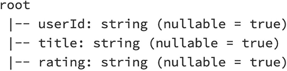
So the preceding output confirms the size of our dataset, and we can then validate the datatypes of the input values to check if we need to change/cast any column datatypes:
[In]: df.printSchema()
[Out]:
There are a total of three columns, and one of them seems to be of the string datatype. We will have to convert it into numerical form to build the recommender system. We now view a few rows of the dataframe using the rand function to shuffle the records in random order:
The movie with the highest number of ratings is Star Wars (1977) and has been rated 583 times, and each movie has been rated by at least one user. We now cast the datatype for the title column. We convert the movie title column from categorical to numerical values using StringIndexer. We import StringIndexer and IndexToString from the PySpark library:
[In]: from pyspark.sql.functions import *
[In]: from pyspark.ml.feature import StringIndexer,IndexToString
Next, we create the StringIndexer object by mentioning the input column and output column. Then we fit the object on the dataframe and apply it on the movie title column to create a new dataframe with numerical values:
Let’s validate the numerical values of the title column by viewing a few rows from the new dataframe (indexed):
[In]: indexed.show(10)
[Out]:
As we can see, now we have an additional column (title_new) with numerical values representing the movie titles. Just to validate the movie counts, we rerun the groupBy function on the new dataframe:
Now that we have prepared the data for building the recommender model, we can split the dataset into training and test sets. We split it in 75/25 ratio to train the model and test its accuracy:
[In]: train,test=indexed.randomSplit([0.75,0.25])
[In]: train.count()
[Out]: 75159
[In]: test.count()
[Out]: 24841
We import the ALS function from PySpark’s ML library and build the model on the training set. There are multiple hyperparameters that can be tuned to improve the performance of the model. Two of the important ones are as follows: nonnegative =‘True’ doesn’t create negative ratings in recommendations, and coldStartStrategy=‘drop’ prevents any NaN rating predictions:
The final part of the entire exercise is to check the performance of the model on unseen or test data. We use the transform function to make predictions on the test data and RegressionEvaluate to check the RMSE value of the model on test data:
[In]: predicted_ratings=rec_model.transform(test)
[In]: predicted_ratings.printSchema()
root
|-- userId: integer (nullable = true)
|-- title: string (nullable = true)
|-- rating: integer (nullable = true)
|-- title_new: double (nullable = false)
|-- prediction: float (nullable = false)
[In]: predicted_ratings.orderBy(rand()).show(10)
[Out]:
[In]: from pyspark.ml.evaluation import RegressionEvaluator
The RMSE is not very high. We are making an error of one point in actual rating and predicted rating. This can be improved further by tuning model parameters and using the hybrid approach. After checking the performance of the model and tuning the hyperparameters, we can move ahead to recommend top movies to users, which they have not seen and might like. The first step is to create a list of unique movies in the dataframe:
So there are a total of 287 unique movies out of 1664 movies that this active user has already rated. So we would want to recommend movies from the remaining 1377 items. We now combine both the tables to find the movies that we can recommend by filtering null values from the joined table:
Finally, we can now make the predictions on this remaining movies dataset for the active user using the recommender model that we built earlier. We filter only the top few recommendations that have the highest predicted ratings:
So movie titles 1277 and 1054 have the highest predicted rating for this active user (85). We can make it more intuitive by adding the movie title back to the recommendations. We use the IndexToString function to create an additional column that returns the movie title:
So the recommendations for the userId (85) are Mina Tannenbaum (1994) and Primary Colors (1998). This can be nicely wrapped in a single function that executes the preceding steps in sequence and generates recommendations for the active user as shown in the following:
#create function to recommend top 'n' movies to any particular user
def top_movies(user_id,n):
"""
This function returns the top 'n' movies that user has not seen yet but might like
"""
#assigning alias name 'a' to unique movies df
a = unique_movies.alias('a')
#creating another dataframe which contains already watched movie by active user
In this chapter, we went over various types of recommendation models along with strengths and limitations of each. We then created a collaborative filtering–based recommender system in PySpark using the ALS method to recommend movies to users.