4

Unpacking, Decryption, and Deobfuscation

In this chapter, we are going to explore different techniques that have been introduced by malware authors to bypass antivirus software static signatures and trick inexperienced reverse engineers. These are mainly, packing, encryption, and obfuscation. We will learn how to identify packed samples, how to unpack them, how to deal with different encryption algorithms – from simple ones, such as sliding key encryption, to more complex algorithms, such as 3DES, AES, and RSA – and how to deal with API encryption, string encryption, and network traffic encryption.

This chapter will help you deal with malware that uses packing and encryption to evade detection and hinder reverse engineering. With the information in this chapter, you will be able to manually unpack malware samples with custom types of packers, understand the malware encryption algorithms that are needed to decrypt its code, strings, APIs, or network traffic, and extract its infiltrated data. You will also understand how to automate the decryption process using IDA Python scripting.

In this chapter, we will cover the following topics:

• Exploring packers
• Identifying a packed sample
• Automatically unpacking packed samples
• Manual unpacking techniques
• Dumping the unpacked sample and fixing the import table
• Identifying simple encryption algorithms and functions
• Advanced symmetric and asymmetric encryption algorithms
• Applications of encryption in modern malware – Vawtrak banking Trojan
• Using IDA for decryption and unpacking

Exploring packers

A packer is a tool that packs together the executable file’s code, data, and sometimes resources, and contains code for unpacking the program on the fly and executing it. Here are some processes we are going to tackle:

• Advanced symmetric and asymmetric encryption algorithms
• Applications of encryption in modern malware – Vawtrak banking Trojan
• Using IDA for decryption and unpacking

Here is a high-level diagram of this process:

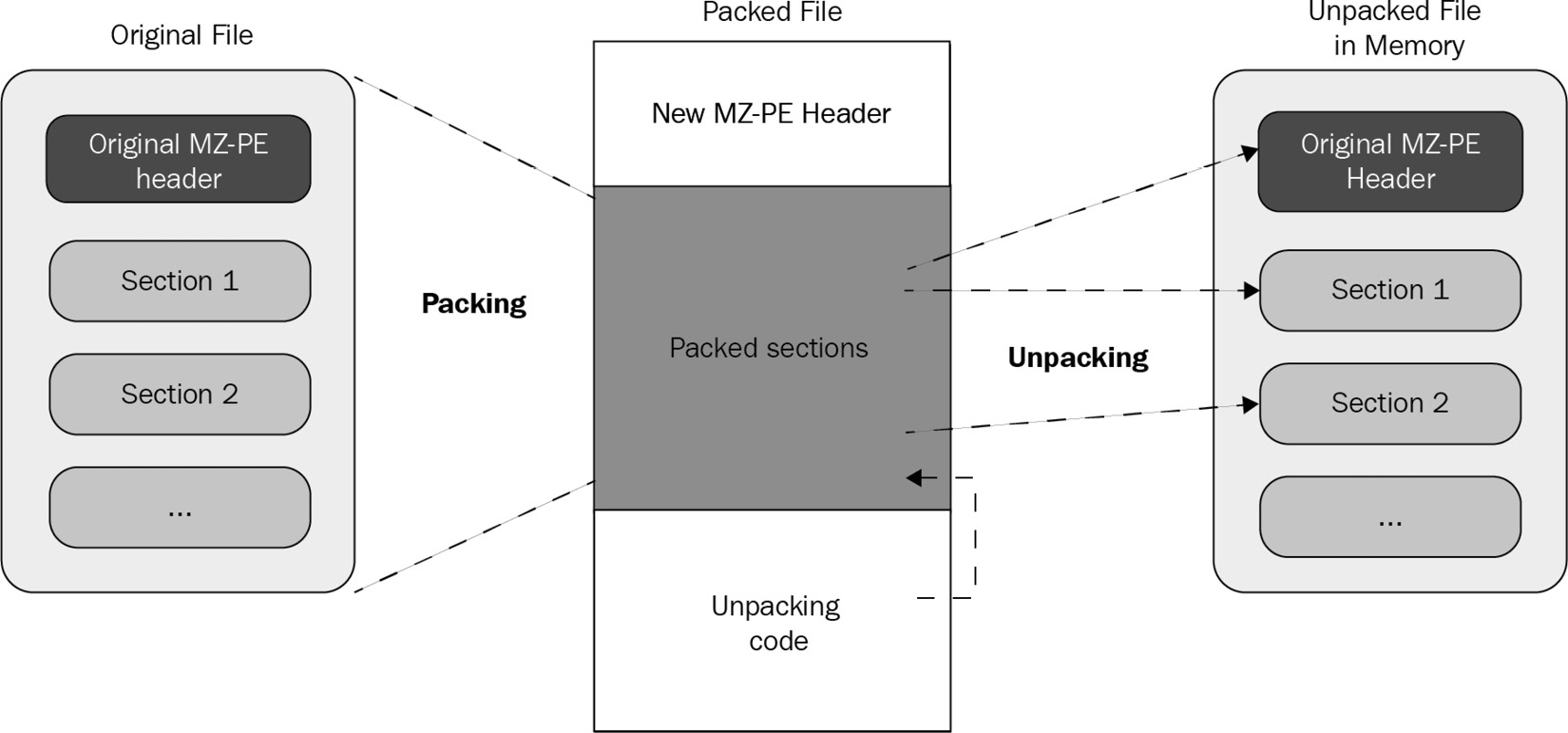
Figure 4.1 – The process of unpacking a sample

Packers help malware authors hide their malicious code behind these compression and/or encryption layers. This code only gets unpacked and executed once the malware is executed (in runtime mode), which helps malware authors bypass static signature-based detections when they are applied against packed samples.

Exploring packing and encrypting tools

Multiple tools can pack/encrypt executable files, but each has a different purpose. It’s important to understand the difference between them as their encryption techniques are customized for the purpose they serve. Let’s go over them:

• Packers: These programs mainly compress executable files, thereby reducing their total size. Since their purpose is compression, they were not created for hiding malicious traits and are not malicious on their own. Therefore, they can’t be indicators that the packed file is likely malicious. There are many well-known packers around, and they are used by both benign software and malware families, such as the following:
  • UPX: This is an open source packer, and its command-line tool can unpack the packed file.
  • ASPack: This is a commonly used packer that has a free and a premium version. The same company that provides ASPack also provides protectors such as ASProtect.
• Legal protectors: The main purpose of these tools is to protect programs against reverse engineering attempts – for example, to protect the licensing system of shareware products or to hide implementation details from competitors. They often incorporate encryption and various anti-reverse engineering tricks. Some of them might be misused to protect malware, but this is not their purpose.
• Malicious encryptors: Similar to legal protectors, their purpose is also to make the analysis process harder; however, the focus here is different: to avoid antivirus detection, you need to bypass sandboxes and hide the malicious traits of a file. Their presence indicates that the encrypted file is more than likely to be malicious as they are not available on the legal market.

In reality, all of these tools are commonly called packers and may include both protection and compression capabilities.

Now that we know more about packers, let’s talk about how to identify them.

Identifying a packed sample

There are multiple tools and multiple ways to identify whether the sample is packed. In this section, we will take a look at different techniques and signs that you can use, from the most straightforward to more intermediate ones.

Technique 1 – using static signatures

The first way to identify whether the malware is packed is by using static signatures. Every packer has unique characteristics that can help you identify it. Some PE tools, such as PEiD and CFF Explorer, can scan the PE file using these signatures or traits and identify the packer that was used to compress the file (if it’s packed); otherwise, they will identify the compiler that was used to compile this executable file (if it’s not packed). The following is an example:

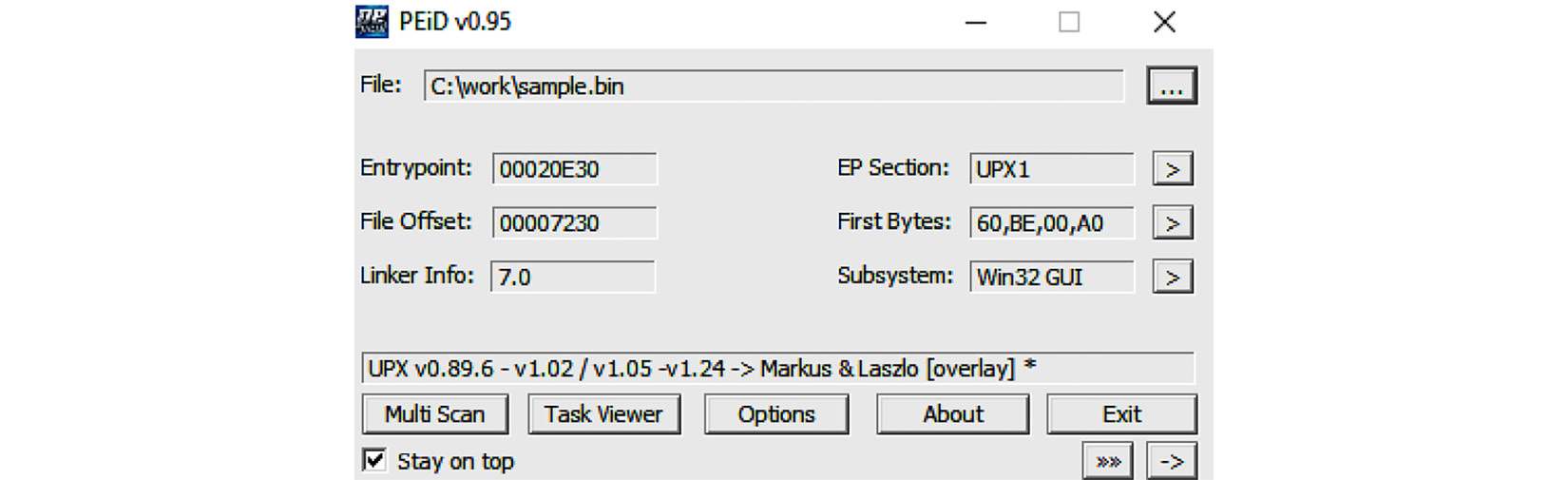
Figure 4.2 – The PEiD tool detecting UPX

All you need to do is open this file in PEiD – you will see the signature that was triggered on this PE file (in the preceding screenshot, it was identified as UPX). However, since they can’t always identify the packer/compiler that was used, you need other ways to identify whether it’s packed and what packer was used, if any.

Technique 2 – evaluating PE section names

Section names can reveal a lot about the compiler or the packer if the file is packed. An unpacked PE file contains sections such as .text, .data, .idata, .rsrc, and .reloc, while packed files contain specific section names, such as UPX0, .aspack, .stub, and so on. Here is an example:

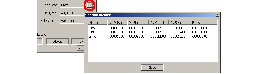
Figure 4.3 – The PEiD tool’s section viewer

These section names can help you identify whether this file is packed. Searching for these section names on the internet could help you identify the packer that uses these names for its packed data or its stub (unpacking code). You can easily find the section names by opening the file in PEiD and clicking on the > button beside EP Section. By doing this, you will see the list of sections in this PE file, as well as their names.

Technique 3 – using stub execution signs

Most packers compress PE file sections, including the code section, data section, import table, and so on, and then add a new section at the end that contains the unpacking code (stub). Since most of the unpacked PE files start the execution from the first section (in most cases, .text), the packed PE files start the execution from one of the last sections, which is a clear indication that a decryption process will be running. The following signs are an indication that this is happening:

• The entry point is not pointing to the first section (it would mostly be pointing to one of the last two sections) and this section’s memory permission is EXECUTE (in the section’s characteristics).
• The first section’s memory permission will be mostly READ | WRITE.

It is worth mentioning that many virus families that infect executable files have similar attributes.

Technique 4 – detecting a small import table

For most applications, the import table is full of APIs from system libraries, as well as third-party libraries; however, in most of the packed PE files, the import table will be quite small and will include a few APIs from known libraries. This is enough to unpack the file. Only one API from each library of the PE file will be used after being unpacked. The reason for this is that most of the packers load the import table manually after unpacking the PE file, as shown in the following screenshot:

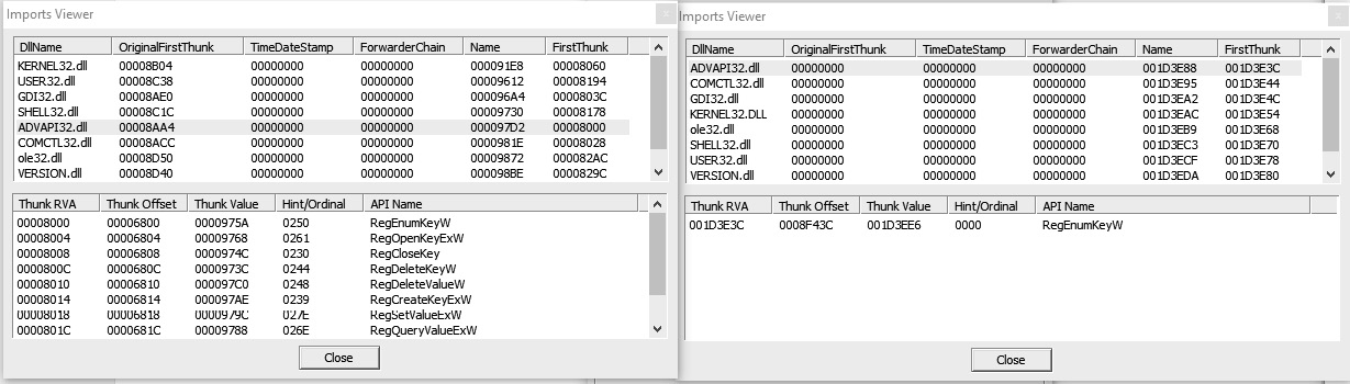
Figure 4.4 – The import table of an unpacked sample versus a packed sample with UPX

The packed sample removed all the APIs from ADVAPI32.dll and left only one, so the library will be automatically loaded by Windows Loader. After unpacking, the unpacker stub code will load all of these APIs again using the GetProcAddress API.

Now that we have a fair idea of how to identify a packed sample, let’s venture forward and explore how to automatically unpack packed samples.

Automatically unpacking packed samples

Before you dive into the manual, time-consuming unpacking process, you need to try some fast automatic techniques first to get a clean unpacked sample in no time at all. In this section, we will explain the most well-known techniques for quickly unpacking samples that have been packed with common packers.

Technique 1 – the official unpacking process

Some packers, such as UPX or WinRAR, are self-extracting packages that include an unpacking technology that’s shipped with the tool. As you may know, these tools are not created to hide any malicious traits, so some of them provide these unpacking features for both developers and end users.

In some cases, malware illegally uses a commercial protector to protect itself from reverse engineering and detection. In this case, you can even directly contact the protection provider to unprotect this piece of malware for your analysis.

In the case of UPX, it is common for attackers to patch the packed sample so that it remains executable, but the standard tool can no longer unpack it. For example, in many cases, it involves replacing the UPX magic value at the beginning of its first section with something else:

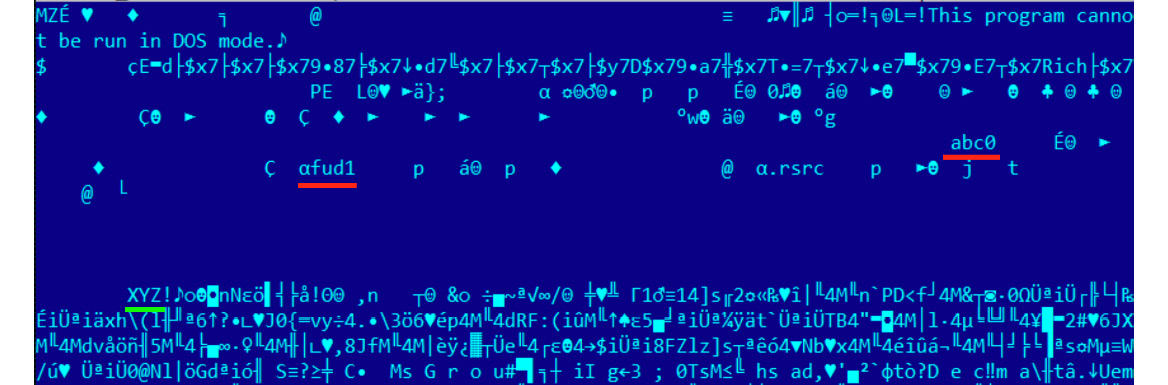
Figure 4.5 – The UPX magic value and section names have changed but the sample remains fully functional

Restoring the original values can make the sample unpackable by a standard tool.

Technique 2 – using OllyScript with OllyDbg

There is an OllyDbg plugin called OllyScript that can help automate the unpacking process. It does this by scripting OllyDbg actions, such as setting a breakpoint, continuing execution, pointing the EIP register to a different place, or modifying some bytes.

Nowadays, OllyScript is not that widely used, but it inspired the next technique.

Technique 3 – using generic unpackers

Generic unpackers are debuggers that have been pre-scripted to unpack specific packers or to automate the manual unpacking process, which we will describe in the next section. Here is an example of one of them:

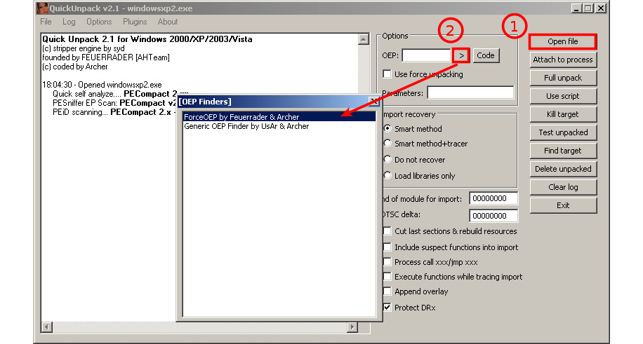
Figure 4.6 – The QuickUnpack tool in detail

They are more generic and can work with multiple packers. However, malware may escape from these tools, which may lead to the malware being executed on the user’s machine. Because of this, you should always use these tools on an isolated virtual machine or in a safe environment.

Technique 4 – emulation

Another group of tools worth mentioning is emulators. Emulators are programs that simulate the execution environment, including the processor (for executing instructions, dealing with registers, and so on), memory, the operating system, and so on.

These tools have more capabilities for running malware safely (as it’s all simulated) and have more control over the execution process. Therefore, they can help set up more sophisticated breakpoints and can also be easily scripted (such as libemu and the Pokas x86 Emulator), as shown in the following code:

from pySRDF import *
emu = Emulator(“upx.exe”)
x = emu.SetBp(“isdirty(eip)”) # which set bp on Execute on modified data
emu.Run() # OR emu.Run(“ins.log”) to log all running instructions
emu.Dump(“upx_unpacked.exe”, DUMP_FIXIMPORTTABLE) # DUMP_FIXIMPORTTABLE create new import table for new API
print(“File Unpacked Successfully

The Disassembled Code
---------------”)

In this example, we used the Pokas x86 Emulator. It was much easier to set more complicated breakpoints, such as Execute on modified data, which gets triggered when the instruction pointer (EIP) is pointing to a decrypted/unpacked place in memory.

Another great example of such a tool based on emulation is unipacker. It is based on the Unicorn engine and supports a decent amount of popular legitimate packers, including ASPack, FSG, MEW, MPRESS, and others.

Technique 5 – memory dumps

The last fast technique we will mention is incorporating memory dumps. This technique is widely used as it’s one of the easiest for most packers and protectors to apply (especially if they have anti-debugging techniques). The idea behind it is to just execute the malware and take a memory snapshot of its process. Some common sandboxing tools provide a process’s memory dump as a core feature or as one of their plugins’ features, such as Cuckoo sandbox.

This technique is very beneficial for static analysis, as well as for static signature scanning; however, the memory dump that is produced is different from the original sample and can’t be executed. Apart from mismatching locations of code and data compared to the offsets specified in the section table, the import table will also need to be fixed before any further dynamic analysis is possible.

Since this technique doesn’t provide a clean sample, and because of the limitations of the previous automated techniques we described, understanding how to unpack malware manually can help you with these special cases that you will encounter from time to time. With manual unpacking, and by understanding anti-reverse engineering techniques (these will be covered in Chapter 6, Bypassing Anti-Reverse Engineering Techniques), you will be able to deal with the most advanced packers.

In the next section, we will explore manual unpacking using OllyDbg.

Manual unpacking techniques

Even though automated unpacking is faster and easier to use than manual unpacking, it doesn’t work with all packers, encryptors, or protectors. This is because some of them require a specific, custom way to unpack. Some of them have anti-VM techniques or anti-reverse engineering techniques, while others use unusual APIs or assembly instructions that emulators can’t detect. In this section, we will look at different techniques for unpacking malware manually.

The main difference between the previous technique and manual unpacking is when we take the memory dump and what we do with it afterward. If we just execute the original sample, dump the whole process memory, and hope that the unpacked module will be available there, we will face multiple problems:

• It is possible that the unpacked sample will already be mapped by sections and that the import table will already have been populated, so the engineer will have to change the physical addresses of each section so that it’s equal to the virtual ones, restore imports, and maybe even handle relocations to make them executable again.
• The hash of this sample will be different from the original one.
• The original loader may unpack the sample to allocated memory, inject it somewhere else, and free the memory so that it won’t be a part of the full dump.
• It is very easy to miss some modules; for example, the original loader may unpack only a sample for either a 32- or 64-bit platform.

The much cleaner way is to stop unpacking when the sample has just been unpacked but hasn’t been used yet. This way, it will just be an original file. In some cases, even its hash will match the original not-yet-packed sample and therefore can be used for threat hunting purposes.

In this section, we will cover several common universal methods of unpacking samples.

Technique 1 – memory breakpoint on execution

This technique works for packers that place an unpacked sample in the same place in memory where the packed file was loaded. As we know, the packed sample will contain sections of the original file (including the code section), and the unpacker stub just unpacks each of them and then transfers control to the original entry point (OEP) for the application to run it normally. This way, we can assume that OEP will be in the first section so that we can set a breakpoint to catch any instructions being executed there. Let’s cover this process step by step.

Step 1 – setting the breakpoints

To intercept the moment when the code in the first section receives control, we can’t use hardware breakpoints on execution as they can be only set to a maximum of four bytes. This way, we would need to know where exactly the execution will start. The more effective solution is to set a memory breakpoint on execution.

The ability to use memory breakpoints on execution is available in OllyDbg implicitly. It can be accessed by going to View | Memory, where we can change the first section’s memory permissions to Read/write if it was Full access. Here is an example:

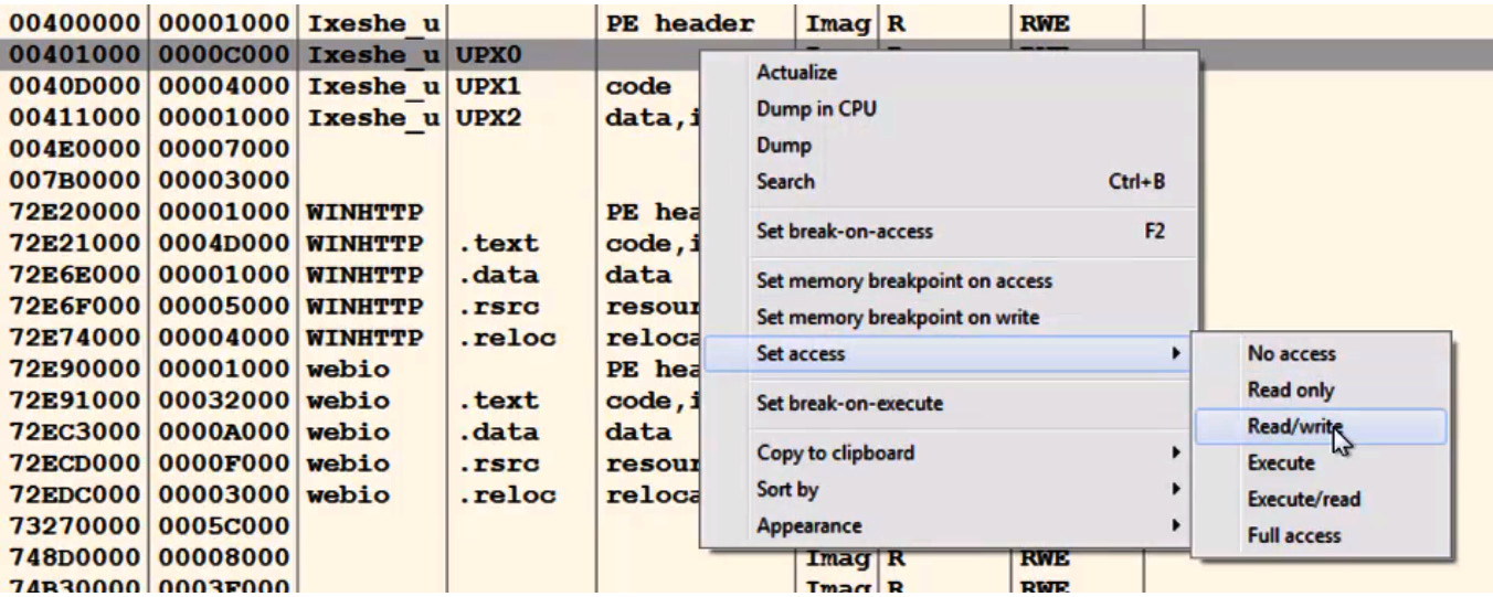
Figure 4.7 – Changing memory permissions in OllyDbg

In this case, we can’t execute code in this section until it gets execute permission. By default, in multiple Windows versions, it will still be executable for noncritical processes, even if the memory permissions don’t include the EXECUTE permission. Therefore, you need to enforce what is called Data Execution Prevention (DEP), which enforces the EXECUTE permission and does not allow any non-executable data to be executed.

This technology is used to prevent exploitation attempts, which we will cover in more detail in Chapter 8, Handling Exploits and Shellcode; however, it comes in handy when we want to unpack malware samples easily.

Step 2 – turning on Data Execution Prevention

To turn on DEP, you can go to Advanced system settings and then Data Execution Prevention. You will need to turn it on for all programs and services, as shown in the following screenshot:

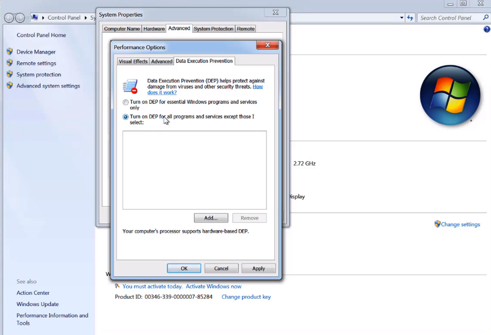
Figure 4.8 – Changing the DEP settings on Windows

Now, these types of breakpoints should be enforced and the malware should be prevented from executing in this section, particularly at the beginning of the decrypted code (OEP).

Step 3 – preventing any further attempts to change memory permissions

Unfortunately, just enforcing DEP is not enough. The unpacking stub can easily bypass this breakpoint by changing the permission of this section to full access again by using the VirtualProtect API.

This API gives the program the ability to change the memory permissions of any memory chunk to any other permissions. You need to set a breakpoint on this API by going to CPU View and right-clicking on the disassemble area. Then, select C | Go To | Expression (or use Ctrl + G), type in the name of the API (in our case, this is VirtualProtect), and set a breakpoint on the address it takes you to.

If the stub tries to call VirtualProtect to change the memory permissions, the debugged process will stop, and you can change the permission it tries to set in the first section. You can change the NewProtect argument value to READONLY or READ|WRITE and remove the EXECUTE bit from it. Here is how it will look in the debugger:

Figure 4.9 – Finding an address that the VirtualProtect API changes permissions for

Once we have handled this part, it is time to let the breakpoint trigger.

Step 4 – executing and getting the OEP

Once you click Run, the debugged process will eventually transfer control to the OEP, which will cause an access violation error to appear, as shown in the following screenshot:

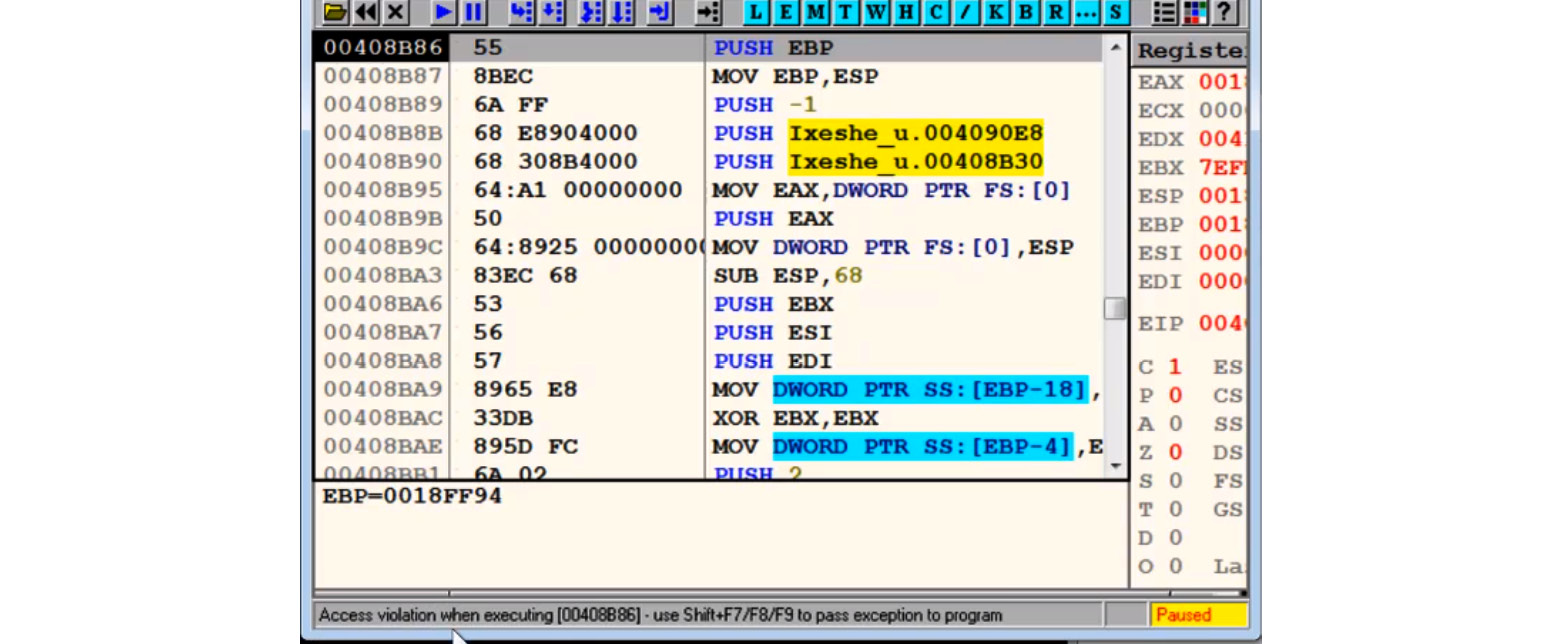
Figure 4.10 – Staying at the OEP of the sample in OllyDbg

This may not happen immediately as some packers modify the first few bytes of the first section with instructions such as ret, jmp, or call, just to make the debugged process break on this breakpoint; however, after a few iterations, the program will break. This occurs after full decryption/decompression of the first section, which it does to execute the original code of the program.

Technique 2 – call stack backtracing

Understanding the concept of the call stack is very useful for speeding up your malware analysis process. First up is the unpacking process.

Take a look at the following code and imagine what the stack will look like:

func01:
1: push ebp
2: mov ebp, esp ; now ebp = esp
...
3: call func02
...
func02:
4: push ebp     ; which was the previous esp before the call
5: mov ebp, esp ; now ebp = new esp
...
6: call func03
...
func03:
7: push ebp     ; which is equal to previous esp
8: mov ebp, esp ; ebp = another new esp
...

When we look at the stack just after the return address saved by call func03, the value of the previous esp is saved using push ebp (it was copied to ebp at line 5). On top of the stack from this previous esp value, the first esp value is stored (this is because instruction 4 of ebp is equal to the first esp value), followed by the return address from call func02, and so on. Here, the stored esp value is followed by a return address. This esp value points to the previously stored esp value, followed by the previous return address, and so on. This is known as a call stack. The following screenshot shows what this looks like in OllyDbg:

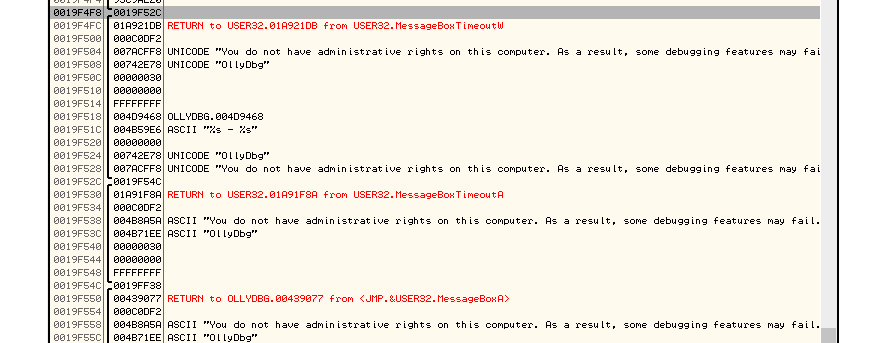
Figure 4.11 – Stored values followed by a return address in OllyDbg

As you can see, the stored esp value points to the next stack frame (another stored esp value and the return address of the previous call), and so on.

OllyDbg includes a view window for the call stack that can be accessed through View | Call Stack. It looks as follows:

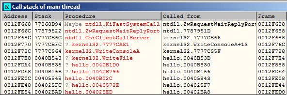
Figure 4.12 – Call stack in OllyDbg

Now, you may be wondering: how can the call stack help us unpack our malware in a fast and efficient way?

Here, we can set a breakpoint that we are sure will make the debugged process break in the middle of the execution of the decrypted code (the actual program code after the unpacking phase). Once the execution stops, we can backtrace the call stack and get to the first call in the decrypted code. Once we are there, we can just slide up until we reach the start of the first function that was executed in the decrypted code, and we can declare this address as the OEP. Let’s describe this process in greater detail.

Step 1 – setting the breakpoints

To apply this approach, you need to set the breakpoints on the APIs that the program will execute at some point. You can rely on the common APIs that are used (examples include GetModuleFileNameA, GetCommandLineA, CreateFileA, VirtualAlloc, HeapAlloc, and memset), your behavioral analysis, or a sandbox report that will give you the APIs that were used during the execution of the sample.

First, you must set a breakpoint on these APIs (use all of your known ones, except the ones that could be used by the unpacking stub) and execute the program until the execution breaks, as shown in the following screenshot:

Figure 4.13 – The return address in the stack window in OllyDbg

Now, you need to check the stack, since most of your next steps will be on the stack side. By doing this, you can start following the call stack.

Step 2 – following the call stack

Follow the stored esp value in the stack and then the next stored esp value until you land on the first return address, as shown in the following screenshot:

Figure 4.14 – The last return address in the stack window in OllyDbg

Now, follow the return address on the disassembled section in the CPU window, as follows:

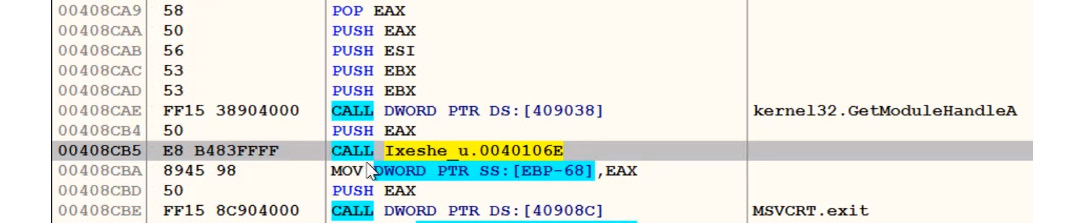
Figure 4.15 – Following the last return address in OllyDbg

Once you have reached the first call in the unpacked section, the only step left is reaching the OEP.

Step 3 – reaching the OEP

Now, you only need to slide up until you reach the OEP. It can be recognized by a standard function prologue, as follows:

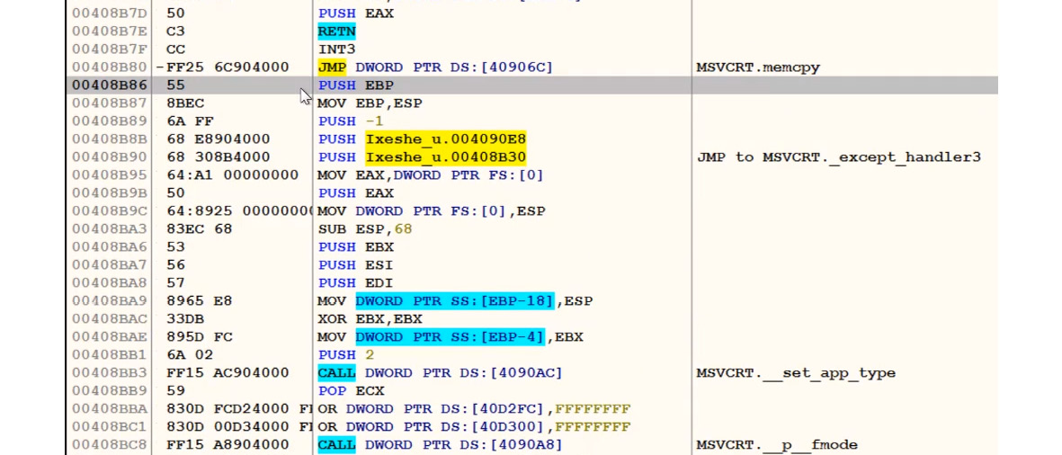
Figure 4.16 – Finding the OEP in OllyDbg

This is the same entry point that we were able to reach using the previous technique. It’s a simple technique to use and it works with many complex packers and encryptors. However, this technique could easily lead to the actual execution of the malware or at least some pieces of its code, so it should be used with care.

Technique 3 – monitoring memory allocated spaces for unpacked code

This method is extremely useful if the time to analyze a sample is limited, or if there are many of them, as here, we are not going into the details of how the original sample is stored.

The idea here is that the original malware usually allocates a big block of memory to store the unpacked/decrypted embedded sample. We will cover what happens when this is not the case later.

There are multiple Windows APIs that can be used for allocating memory in user mode. Attackers generally tend to use the following ones:

• VirtualAlloc/VirtualAllocEx/VirtualAllocExNuma
• LocalAlloc/GlobalAlloc/HeapAlloc
• RtlAllocateHeap

In kernel mode, there are other functions such as ZwAllocateVirtualMemory; ExAllocatePoolWithTag can be used in pretty much the same way.

If the sample is written in C, it makes sense to monitor malloc/calloc functions straight away. For C++ malware, we can also monitor the new operator.

Once we have stopped at the entry point of the sample (or at the beginning of the TLS routine, if it is available), we can set a breakpoint on execution at these functions. Generally, it is OK to put a breakpoint on the first instruction of the function, but if there is a concern that malware can hook it (that is, replace the first several bytes with some custom code), the breakpoint at the last instruction will work better.

Another advantage of this is that this way, it only needs one breakpoint for both VirtualAllocEx and VirtualAlloc (which is a wrapper around the former API). In the IDA debugger, it is possible to go to the API by pressing the G hotkey and prefixing the API name with the corresponding DLL without the file extension and separating it with an underscore, for example, kernel32_VirtualAlloc, as shown in the following screenshot:

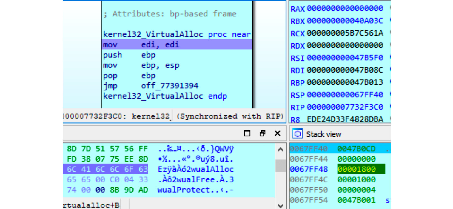
Figure 4.17 – Setting a breakpoint at memory allocation in WinAPI

After this, we continue execution and keep monitoring the sizes of the allocated blocks. So long as it is big enough, we can put a breakpoint on the write operation to intercept the moment when the encrypted (or already decrypted on the fly) payload is being written there. If the malware calls one of these functions too many times, it makes sense to set a conditional breakpoint and monitor only allocations of blocks bigger than a particular size. After this, if the block is still encrypted, we can keep a breakpoint on write and wait until the decryption routine starts processing it. Finally, we can dump the memory block to disk when the last byte is decrypted.

Other API functions that can be used in the same approach include the following:

• VirtualProtect: Malware authors can use this to make the memory block store the unpacked sample executable or make the header or the code section non-writeable.
• WriteProcessMemory: This is often used to inject the unpacked payload, either into some other process or into itself.

Some packers, such as UPX, follow a slightly different approach by having an entry in their section table with a section that takes a lot of space in RAM but is not present on a disk (having a physical size equal to 0). This way, the Windows Loader will prepare this space for the unpacker for free without any need for it to allocate memory dynamically. In this case, placing a breakpoint on write at the beginning of this section will work the same way as described previously.

In most cases, malware unpacks the whole sample at once so that after dumping it, we get the correct MZ-PE file, which can be analyzed independently. However, other options exist, such as the following:

• A decrypted block is a corrupted executable and depends on the original packer to perform correctly.
• The packer decrypts the sample section by section and loads each of them one by one. There are many ways this can be handled, as follows:
  • Dump sections, so long as they become available, and concatenate them later.
  • Modify the decryption routine to process the whole sample at once.
  • Write a script that decrypts the whole encrypted block.

If the malicious program terminates at any stage, it might be a sign that it either needs something extra (such as command-line arguments or an external file, or perhaps it needs to be loaded in a specific way) or that an anti-reverse engineering trick needs to be bypassed. You can confirm this in many ways – for example, by intercepting the moment when the program is going to terminate (for example, by placing a breakpoint on ExitProcess, TerminateProcess, or the more fancy PostQuitMessage API call) and tracing which part of the code is responsible for it. Some engineers prefer to go through the main function manually, step by step – without going into subroutines until one of them causes a termination – and then restart the process and trace the code of this routine. Then, we can trace the code of the routine inside it, if necessary, right up until the moment the terminating logic is confirmed.

Technique 4 – in-place unpacking

While not common, it is possible to either decrypt the sample in the same section where it was originally located (this section should have WRITE|EXECUTE permissions) or in another section of an original file.

In this case, it makes sense to perform the following steps:

1. Search for a big encrypted block (usually, it has high entropy and is visible to the naked eye in a hex editor).
2. Find the exact place where it will be read (the first bytes of the block may serve other purposes – for example, they may store various types of metadata, such as sizes or checksums/hashes, to verify the decryption).
3. Put a breakpoint on read and/or write there.
4. Run the program and wait for the breakpoint to be triggered.

So long as this block is accessed by the decryption routine, it is pretty straightforward to get the decrypted version of it – either by placing a breakpoint on execution at the end of the decryption function or a breakpoint on write to the last bytes of the encrypted block to intercept the moment when they are processed.

It is worth mentioning that this approach can be used together with the one that relies on malware allocating memory. This will be discussed in the Manual unpacking techniques section.

Technique 5 – searching for and transferring control to OEP

In theory, any control flow instruction can be used to transfer control to the OEP once the unpacking is done. However, in reality, many unpackers just use the jmp instruction as they don’t need any conditions and they don’t need to get the control back (another less common option is using a combination of push <OEP_addr> and ret). As the address of the OEP is often not known at compilation time, it is generally passed to jmp in the form of a register or a value stored at a particular offset rather than an actual virtual address and therefore easy to spot. Another option might be that the OEP address is known at compilation time, but there is no code there yet as the unpacking hasn’t finished yet. In both cases, searching for anomalous control transfer instructions may be a quick way to spot the OEP. In the case of jmp, it can be done by running a full-text search for all jmp instructions (In IDA, you can use the Alt + T hotkey combination) and sorting them to spot anomalous entries. Here is an example of such a control transfer:

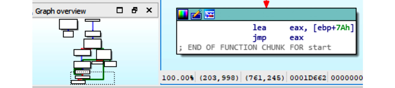
Figure 4.18 – Uncommon control transfer involving a register

Now let’s move on to technique 6.

Technique 6 – stack restoration-based

This technique is usually quicker to do than the previous two, but it is less reliable. The idea here is that some packers will transfer control to the unpacked code at the end of the main function when the unpacking is done. We already know that, at the end of the function, the stack pointer is returned to the same address that it had at the beginning of this function. In this case, it is possible to set a breakpoint on access to the [esp-4]/[rsp-8] value while staying at the entry point of the sample and then execute it so that the breakpoint will hopefully trigger just before it transfers control to the unpacked code.

This may never happen, depending on the implementation of the unpacking code, and there may be other situations where this does happen (for example, when there are multiple garbage calls before starting the actual unpacking process). Therefore, this method can only be used as a first quick check before more time is spent on the other methods.

After we reach the point where we have the unpacked sample in memory, we need to save it to disk. In the next section, we will describe how to dump the unpacked malware from memory to disk and fix the import table.

Dumping the unpacked sample and fixing the import table

In this section, we will learn how to dump the unpacked malware in memory to disk and fix its import table. In addition to this, if the import table has already been populated with API addresses by the loader, we will need to restore the original values. In this case, other tools will be able to read it, and we will be able to execute it for dynamic analysis.

Dumping the process

To dump the process, you can use OllyDump. OllyDump is an OllyDbg plugin that can dump the process back to an executable file. It unloads the PE file back from memory into the necessary file format:

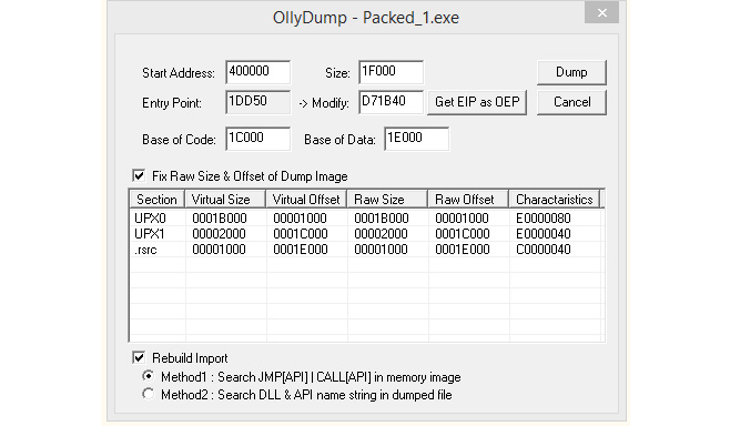
Figure 4.19 – The OllyDump UI

Once you reach the OEP from the previous manual unpacking process, you can set the OEP as the new entry point. OllyDump can fix the import table (as we will soon describe). You can either use it or uncheck the Rebuild Import checkbox if you are willing to use other tools.Another option is to use tools such as PETools or Lord PE for 32-bit and VSD for both 32- and 64-bit Windows. The main advantage of these solutions is that apart from the so-called Dump Full option, which mainly dumps original sections associated with the sample, it is also possible to dump a particular memory region – for example, allocated memory with the decrypted/unpacked sample(s), as shown in the following screenshot:

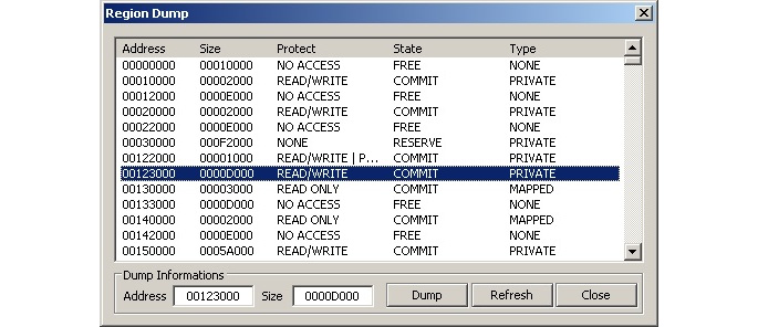
Figure 4.20 – The Region Dump window of PETools

Next, we are going to look at fixing the import table of a piece of malware.

Fixing the import table

Now, you may be wondering: what happens to the import table that needs to be fixed? The answer is: when the PE file gets loaded in the process memory or the unpacker stub loads the import table, the loader goes through the import table (you can find more information in Chapter 3, Basic Static and Dynamic Analysis for x86/x64) and populates it with the actual addresses of API functions from DLLs that are available on the machine. Here is an example:

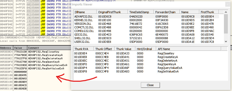
Figure 4.21 – The import table before and after PE loading

After this, these API addresses are used to access these APIs throughout the application code, usually by using the call and jmp instructions:

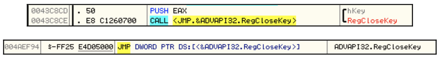
Figure 4.22 – Examples of different API calls

To restore the import table, we need to find this list of API addresses, find which API each address represents (we need to go through each library list of addresses and their corresponding API names for this), and then replace each of these addresses with either an offset pointing to the API name string or an ordinal value. If we don’t find the API names in the file, we may need to create a new section that we can add these API names to and use them to restore the import table.

Fortunately, some tools do this automatically. In this section, we will talk about Import REConstructor (ImpREC). Here is what it looks like:

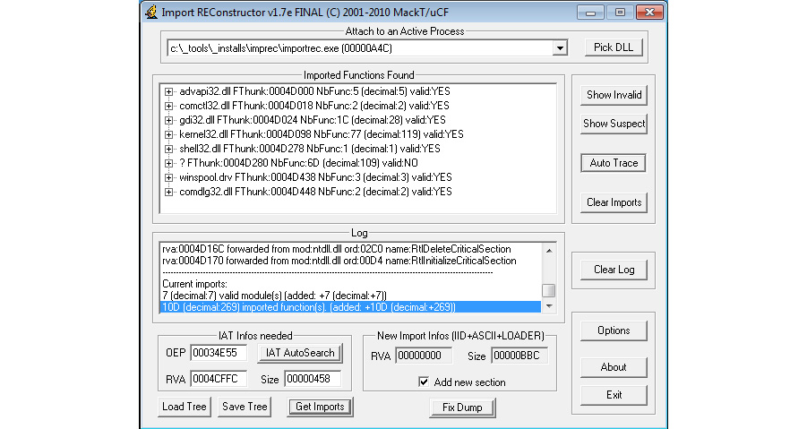
Figure 4.23 – The ImpREC interface

To fix the import table, you need to follow these steps:

1. Dump the process or any library you want to dump using, for example, OllyDump (and uncheck the Rebuild Import checkbox) or any other tool of preference.
2. Open ImpREC and choose the process you are currently debugging.
3. Now, set the OEP value to the correct value and click on IAT AutoSearch.
4. After that, click on Get Imports and delete any rows with valid: NO from the Imported Functions Found section.
5. Click on the Fix Dump button and then select the previously dumped file. Now, you will have a working, unpacked PE file. You can load it into PEiD or any other PE explorer application to check whether it is working.

Important Note

For a 64-bit Windows system, the Scylla or CHimpREC tools can be used instead.

In the next section, we will discuss basic encryption algorithms and functions to strengthen our knowledge base and thus enrich our malware analysis capabilities.

Identifying simple encryption algorithms and functions

In this section, we will take a look at the simple encryption algorithms that are widely used in the wild. We will learn about the difference between symmetric and asymmetric encryption, and we will learn how to identify these encryption algorithms in the malware’s disassembled code.

Types of encryption algorithms

Encryption is the process of modifying data or information to make it unreadable or unusable without a secret key, which is only given to people who are expected to read the message. The difference between encoding or compression and encryption is that they do not use any key, and their main goal is not related to protecting the information or limiting access to it compared to encryption.

There are two basic types of encryption algorithms: symmetric and asymmetric (also called public-key algorithms). Let’s explore the differences between them:

• Symmetric algorithms: These types of algorithms use the same key for encryption and decryption. They use a single secret key that’s shared by both sides:

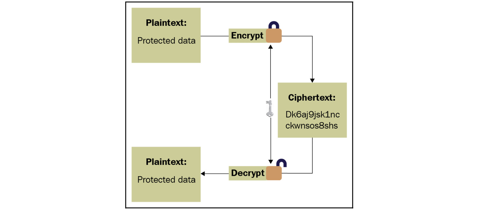
Figure 4.24 – Symmetric algorithm explained

• Asymmetric algorithms: In this case, two keys are used. One is used for encryption and the other is used for decryption. These two keys are called the public key and the private key. One key is shared publicly (the public key), while the other one is kept secret (the private key). Here is a high-level diagram describing this process:

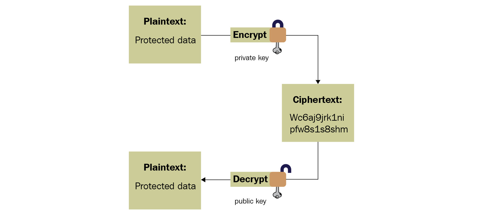
Figure 4.25 – Asymmetric algorithm explained

Now, let’s talk about simple custom-made encryption algorithms commonly used in malware.

Basic encryption algorithms

Most encryption algorithms that are used by malware consist of basic mathematical and logical instructions – that is, xor, add, sub, rol, and ror. These instructions are reversible, and you don’t lose data while encrypting with them compared to instructions such as shl or shr, where it is possible to lose some bits from the left and right. This also happens with the and and or instructions, which can lead to data loss when using or with 1 or and with 0.

These operations can be used in multiple ways, as follows:

• Simple static encryption: Here, the malware just uses the aforementioned operations to change the data using the same key. Here is an example of it that uses the rol instruction:

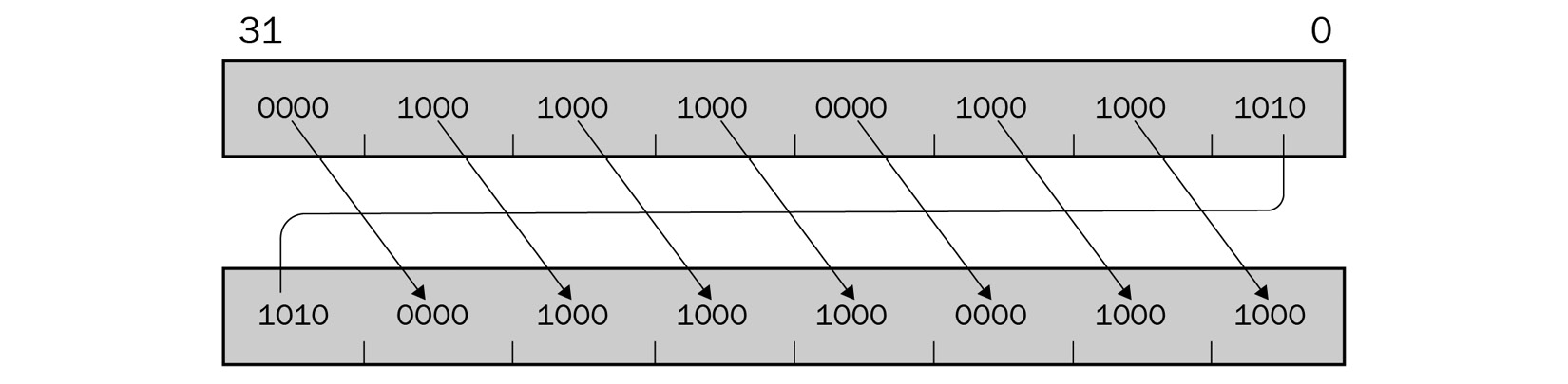
Figure 4.26 – Example of the rol instruction

• Running key encryption: Here, the malware changes the key during the encryption. Here is an example:

  loop_start:

  mov edx, <secret_key>

  xor dword ptr [<data_to_encrypt> + eax], edx

  add edx, 0x05 ; add 5 to the key

  inc eax

  loop loop_start

• Substitutional key encryption: Malware can substitute bytes with each other or substitute each value with another value (for example, for each byte with a value of 0x45, the malware could change this value to 0x23).
• Other encryption algorithms: Malware authors never run out of ideas when it comes to creating new algorithms that represent a combination of these arithmetic and logical instructions. This leads us to the next question: how can we identify encryption functions?

Identifying encryption functions in disassembly

The following screenshot demonstrates sections that have been numbered from 1 to 4. These sections are key to understanding and identifying the encryption algorithms that are used in malware:

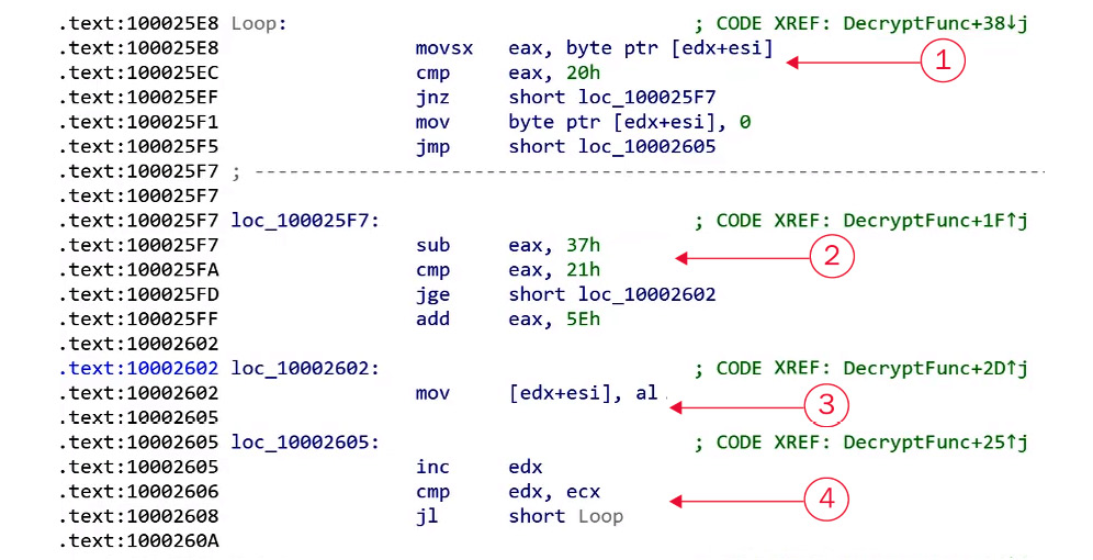
Figure 4.27 – Things to pay attention to when identifying the encryption algorithm

To identify an encryption function, there are four things you should be searching for, as shown in the following table:

These four points are the core parts of any encryption loop. They can easily be spotted in a small encryption loop but may be harder to spot in a more complicated encryption loop such as RC4 encryption, which we will discuss later.

String search detection techniques for simple algorithms

In this section, we will be looking into a technique called X-RAYING (first introduced by Peter Ferrie in the PRINCIPLES AND PRACTISE OF X-RAYING article in VB2004). This technique is used by antivirus products and other static signature tools to detect samples with signatures, even if they are encrypted. This technique can dig under the encryption layers to reveal the sample code and detect it without knowing the encryption key in the first place and without incorporating time-consuming techniques such as brute-forcing. Here, we will describe the theory and the applications of this technique, as well as some of the tools we can use to help us use it. We may use this technique to detect embedded PE files or decrypt malicious samples.

The basics of X-RAYING

For the types of algorithms that we described earlier, if you have the encrypted data, the encryption algorithm, and the secret key, you can easily decrypt the data (which is the purpose of all encryption algorithms); however, if you have the encrypted data (ciphertext) and a piece of the decrypted data, can you still decrypt the remaining parts of the encrypted data?

In X-RAYING, you can brute-force the algorithm and its secret key(s) if you have a piece of decrypted data (plaintext), even if you don’t know the offset of this plain text data in the whole encrypted blob. It works on almost all the simple algorithms that we described earlier, even with multiple layers of encryption. For most of the encrypted PE files, the plain text includes strings such as This program cannot run in DOS mode or kernel32.dll, as well as arrays of null bytes.

First of all, we will choose the first candidate to be an encryption algorithm, for example, XOR. Then, we will search for a part of the plain text inside ciphertext. To do that, we will use a part of the expected plain text to XOR it against the ciphertext, for example, a 4-byte string. The result of XORing will give us a candidate decryption key (a property of the XOR algorithm). Then, we will test this key with the remaining plain text. If this key works, it will reveal the remaining plain text of the ciphertext, which means that we will have found the secret key and can decrypt the remaining data.

Now, let’s talk about various tools that may help us speed up this process.

X-RAYING tools for malware analysis and detection

Some tools have been written to help malware researchers use the X-RAYING technique for scanning. The following are some of these tools that you can use, either from the command line or by using a script:

• XORSearch: This is a tool that was created by Didier Stevens, and it searches inside ciphertext by using a given plain text sample to search for. It doesn’t only cover XOR – it also covers other algorithms, including bit shifting (based on the rol and ror instructions):

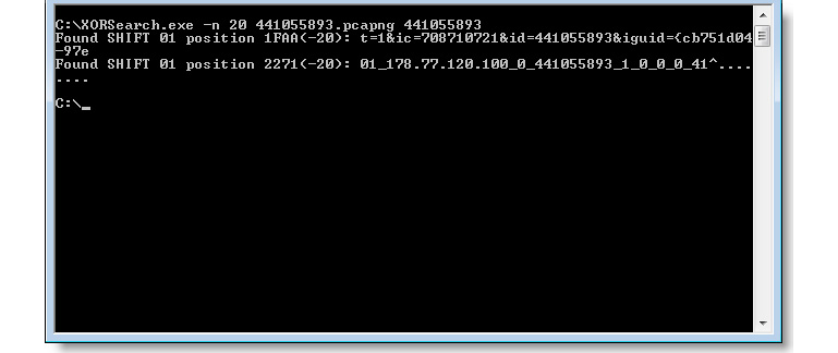
Figure 4.28 – The XORSearch UI

• Yara Scanner: Yara is a static signature tool that helps scan files with predefined signatures. It allows regex, wildcard, and other types of signatures. It also allows xor signatures:

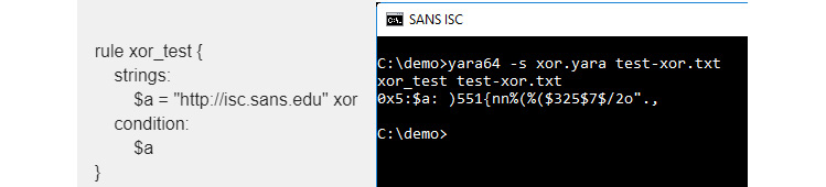
Figure 4.29 – Example of using a YARA signature

For more advanced X-RAYING techniques, you may need to write a small script to scan with manually.

Identifying the RC4 encryption algorithm

The RC4 algorithm is one of the most common encryption algorithms that is used by malware authors, mainly because it is simple and, at the same time, strong enough to not be broken like other simple encryption algorithms. Malware authors generally implement it manually instead of relying on WinAPIs, which makes it harder for novice reverse engineers to identify. In this section, we will see what this algorithm looks like and how you can spot it.

The RC4 encryption algorithm

The RC4 algorithm is a symmetric stream algorithm that consists of two parts: a key-scheduling algorithm (KSA) and a pseudo-random generation algorithm (PRGA). Let’s have a look at each of them in greater detail.

The key-scheduling algorithm

The key-scheduling part of the algorithm creates an array of 256 bytes called an S array from the secret key. This array will be used to initialize the stream key generator. This consists of two parts:

• It creates an S array with values from 0 to 256 sequentially:

  for i from 0 to 255

    S[i] := i

  endfor

• It permutates the S array using key material:

  for i from 0 to 255

    j := (j + S[i] + key[i mod keylength]) mod 256

    swap values of S[i] and S[j]

  endfor

Once this initiation part for the key is done, the decryption algorithm starts. In most cases, the KSA part is written in a separate function that takes only the secret key as an argument, without the data that needs to be encrypted or decrypted.

Pseudo-random generation algorithm (PRNG)

The pseudo-random generation part of the algorithm just generates pseudo-random values (again, based on swapping bytes, as we did for the S array), but also performs an XOR operation with the generated value and a byte from the data:

i := 0
j := 0
while GeneratingOutput:
  i := (i + 1) mod 256
  j := (j + S[i]) mod 256
  swap values of S[i] and S[j]
  K := S[(S[i] + S[j]) mod 256]
  Data[i] = Data[i] xor K
endwhile

As you can see, the actual encryption algorithm that was used was xor. However, all this swapping aims to generate a different key value every single time (similar to sliding key algorithms).

Identifying RC4 algorithms in a malware sample

To identify an RC4 algorithm, some key characteristics can help you detect it:

• The generation of the 256 bytes array: This part is easy to recognize, and it’s unique for a typical RC4 algorithm like this:

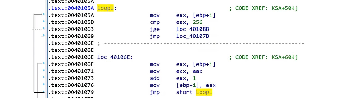
Figure 4.30 – Array generation in the RC4 algorithm

• There’s lots of swapping: If you can recognize the swapping function or code, you will find it everywhere in the RC4 algorithm. The KSA and PRGA parts of the algorithm are a good sign that it is an RC4 algorithm:

Figure 4.31 – Swapping in the RC4 algorithm

• The actual algorithm is XOR: At the end of a loop, you will notice that this algorithm is an XOR algorithm. All the swapping is done on the key. The only changes that affect the data are done through XOR:

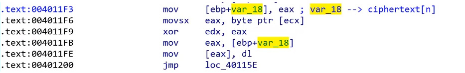
Figure 4.32 – The XOR operation in the RC4 algorithm

• Encryption and decryption similarity: You will also notice that the encryption and the decryption functions are the same functions. The XOR logical gate is reversible. You can encrypt the data with XOR and the secret key and decrypt this encrypted data with XOR and the same key (which is different from the add/sub algorithms, for example).

Now, it is time to talk about more complex algorithms.

Advanced symmetric and asymmetric encryption algorithms

Standard encryption algorithms such as symmetric DES and AES or asymmetric RSA are widely used by malware authors. However, the vast majority of samples that include these algorithms never implement these algorithms themselves or copy their code into their malware. They are generally implemented using Windows APIs.

These algorithms are mathematically more complicated than simple encryption algorithms or RC4. While you don’t necessarily need to understand their mathematical background to understand how they are implemented, it is important to know how to identify the way they can be used and how to figure out the exact algorithm involved, the encryption/decryption key(s), and the data.

Extracting information from Windows cryptography APIs

Some common APIs are used to provide access to cryptographic algorithms, including DES, AES, RSA, and even RC4 encryption. Some of these APIs are CryptAcquireContext, CryptCreateHash, CryptHashData, CryptEncrypt, CryptDecrypt, CryptImportKey, CryptGenKey, CryptDestroyKey, CryptDestroyHash, and CryptReleaseContext (from Advapi32.dll).

Here, we will take a look at the steps malware has to go through to encrypt or decrypt its data using any of these algorithms and how to identify the exact algorithm that’s used, as well as the secret key.

Step 1 – initializing and connecting to the cryptographic service provider (CSP)

The cryptographic service provider is a library that implements cryptography-related APIs in Microsoft Windows. For the malware sample to initialize and use one of these providers, it executes the CryptAcquireContext API, as follows:

CryptAcquireContext(&hProv,NULL,MS_STRONG_PROV,PROV_RSA_FULL,0);

You can find all the supported providers in your system in the registry in the following key:

HKEY_LOCAL_MACHINESOFTWAREMicrosoftCryptographyDefaultsProvider

Step 2 – preparing the key

There are two ways to prepare the encryption key. As you may know, the encryption keys for these algorithms are usually of a fixed size. Here are the steps that malware authors commonly take to prepare the key:

1. First, the author uses their plain text key and hashes it using any of the known hashing algorithms, such as MD5, SHA128, SHA256, or others:

   CryptCreateHash(hProv,CALG_MD5,0,0,&hHash); CryptHashData(hHash,secretkey,secretkeylen,0);

2. Then, they create a session key from this hash using CryptDeriveKey, like so:

   CryptDeriveKey(hProv, CALG_3DES, hHash, 0, &hKey);

From here, they can easily identify the algorithm from the second argument value that’s provided to this API. The most common algorithms/values are as follows:

CALG_DES = 0x00006601  // DES encryption algorithm.

CALG_3DES = 0x00006603 // Triple DES encryption algorithm.

CALG_AES = 0x00006611  // Advanced Encryption Standard (AES).

CALG_RC4 = 0x00006801   // RC4 stream encryption algorithm.

CALG_RSA_KEYX = 0x0000a400 // RSA public key exchange algorithm.

3. Some malware authors use a KEYBLOB, which includes their key, along with CryptImportKey. A KEYBLOB is a simple structure that contains the key type, the algorithm that was used, and the secret key for encryption. The structure of a KEYBLOB is as follows:

   typedef struct KEYBLOB { BYTE bType;

   BYTE bVersion; WORD reserved; ALG_ID aiKeyAlg; DWORD KEYLEN;

   BYTE[] KEY;}

The bType phrase represents the type of this key. The most common types are as follows:

• PLAINTEXTKEYBLOB (0x8): States a plain text key for a symmetric algorithm, such as DES, 3DES, or AES
• PRIVATEKEYBLOB (0x7): States that this key is the private key of an asymmetric algorithm
• PUBLICKEYBLOB (0x6): States that this key is the public key of an asymmetric algorithm

The aiKeyAlg phrase includes the type of the algorithm as the second argument of CryptDeriveKey. Some examples of this KEYBLOB are as follows:

BYTE DesKeyBlob[] = { 0x08,0x02,0x00,0x00,0x01,0x66,0x00,0x00, // BLOB header 0x08,0x00,0x00,0x00, // key length, in bytes
0xf1,0x0e,0x25,0x7c,0x6b,0xce,0x0d,0x34 // DES key with parity
};

As you can see, the first byte (bType) shows us that it’s a PLAINTEXTKEYBLOB, while the algorithm (0x01,0x66) represents CALG_DES (0x6601).

Another example of this is as follows:

BYTE rsa_public_key[] = {
0x06, 0x02, 0x00, 0x00, 0x00, 0xa4, 0x00, 0x00,
0x52, 0x53, 0x41, 0x31, 0x00, 0x08, 0x00, 0x00,
...
}

This represents a PUBLICKEYBLOB (0x6), while the algorithm represents CALG_RSA_KEYX (0xa400). After that, they are loaded via CryptImportKey:

CryptImportKey(akey->prov, (BYTE *) &key_blob, sizeof(key_blob), 0, 0, &akey->ckey)

Here is an example of how this looks in assembly:

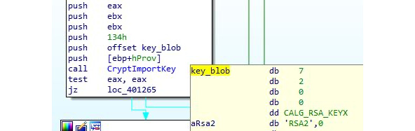
Figure 4.33 – The CryptImportKey API is being used to import an RSA key

Once the key is ready, it can be used for encryption and decryption purposes.

Step 3 – encrypting or decrypting the data

Now that the key is ready, the malware uses CryptEncrypt or CryptDecrypt to encrypt or decrypt the data, respectively. With these APIs, you can identify the start of the encrypted blob (or the blob to be encrypted). These APIs are used like this:

CryptEncrypt(hKey,NULL,1,0,cyphertext,ctlen,sz); CryptDecrypt(hKey,NULL,1,0,plaintext,&ctlen);

Step 4 – freeing the memory

This is the last step, where we free the memory and all the handles that have been used by using the CryptDestroyKey APIs.

Cryptography API: Next Generation (CNG)

There are other ways to implement these encryption algorithms. One of them is by using Cryptography API: Next Generation (CNG), which is a new set of APIs that has been implemented by Microsoft. Still not widely used in malware, they are much easier to understand and extract information from. The steps for using them are as follows:

1. Initialize the algorithm provider: In this step, you can identify the exact algorithm (check MSDN for the list of supported algorithms):

   BCryptOpenAlgorithmProvider(&hAesAlg, BCRYPT_AES_ALGORITHM, NULL, 0)

2. Prepare the key: This is different from preparing a key in symmetric and asymmetric algorithms. This API may use an imported key or generate a key. This can help you extract the secret key that’s used for encryption, like so:

   BCryptGenerateSymmetricKey(hAesAlg, &hKey, pbKeyObject, cbKeyObject, (PBYTE)SecretKey, sizeof(SecretKey), 0)

3. Encrypt or decrypt data: In this step, you can easily identify the start of the data blob to be encrypted (or decrypted):

   BCryptEncrypt(hKey, pbPlainText, cbPlainText, NULL, pbIV, cbBlockLen, NULL, 0, &cbCipherText, BCRYPT_BLOCK_PADDING)

4. Cleanup: This is the last step, and it uses APIs such as BCryptCloseAlgorithmProvider, BCryptDestroyKey, and HeapFree to clean up the data.

Now, let’s see how all this knowledge will help us understand malware’s functionality.

Applications of encryption in modern malware – Vawtrak banking Trojan

In this chapter, we have seen how encryption or packing is used to protect the whole malware. Here, we will look at other implementations of these encryption algorithms inside the malware code for obfuscation and for hiding malicious key characteristics. These key characteristics can be used to identify the malware family using static signatures or even network signatures.

In this section, we will take a look at a known banking trojan called Vawtrak. We will see how this malware family encrypts its strings and API names and obfuscates its network communication.

String and API name encryption

Vawtrak implements a quite simple encryption algorithm. It’s based on sliding key algorithm principles and uses subtraction as its main encryption technique. Its encryption looks like this:

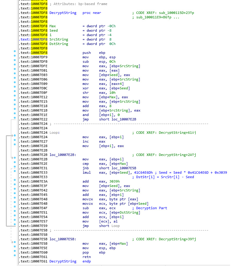
Figure 4.34 – Encryption loop in the Vawtrak malware

The encryption algorithm consists of two parts:

• Generating the next key: This generates a 4-byte number (called a seed) and uses only 1 byte of it as a key:

  seed = ((seed * 0x41C64E6D) + 0x3039 ) & 0xFFFFFFFF key = seed & 0xFF

• Encrypting the data: This part is very simple as it encrypts the data using the following logic:

  data[i] = data[i] - eax

This encryption algorithm is used to encrypt API names and DLL names so that after decryption, the malware can load the DLL dynamically using an API called LoadLibrary, which loads a library if it wasn’t loaded or just gets its handle if it’s already loaded.

After getting the DLL address, the malware gets the API address to execute using an API called GetProcAddress, which gets this function address by the handle for the library and the API name. The malware implements it as follows:

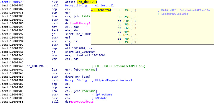
Figure 4.35 – Resolving API names in the Vawtrak malware

The same function (DecryptString) is used a lot inside the malware to decrypt each string on demand (only when it’s being used), as follows:

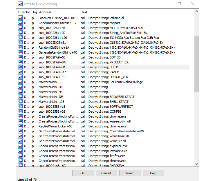
Figure 4.36 – The xrefs to decryption routine in Vawtrak malware

To decrypt this, you need to go through each call to the decrypt function being called and pass the address of the encrypted string to decrypt it. This may be exhausting or time-consuming, so automation (for example, using IDA Python or a scriptable debugger/emulator) could help, as we will see in the next section.

Network communication encryption

Vawtrak can use different encryption algorithms to encrypt its network communications. It implements multiple algorithms, including RC4, LZMA compression, the LCG encryption algorithm (this is used with strings, as we mentioned in the previous section), and others. In this section, we will take a look at the different parts of its encryption.

Inside the requests, it has implemented some encryption to hide basic information, including CAMPAIGN_ID and BOT_ID, as shown in the following screenshot:

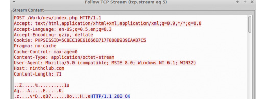
Figure 4.37 – The network traffic of the Vawtrak malware

The cookie, or PHPSESSID, included an encryption key. The encryption algorithm that was used was RC4 encryption. Here is the message after decryption:

Figure 4.38 – Extracted information from the network traffic of the Vawtrak malware

The decrypted PHPSESSID includes the RC4 key in the first 4 bytes. BOT_ID and the next byte represent Campaign_Id (0x03), while the remaining ones represent some other important information.

The data that’s received is in the following structure and includes the first seed that will be used in decryption, the total size, and multiple algorithms that are used to decrypt them:

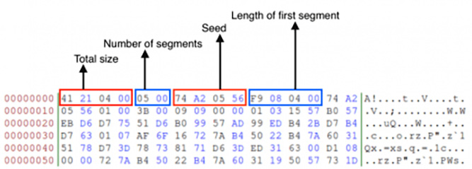
Figure 4.39 – The structure that’s used for decryption in the Vawtrak malware

Unfortunately, with network communication, there’s no simple way to grab the algorithms that were used or the protocol’s structure. You have to search for network communication functions such as HttpAddRequestHeadersA (the one we saw in the decryption process earlier) and other network APIs and trace the data that was received, as well as trace the data that’s going to be sent, until you find the algorithms and the structure behind the command-and-control communication.

Now, let’s explore various capabilities of IDA that may help us understand and circumvent the encryption and packing techniques involved.

Using IDA for decryption and unpacking

IDA is a very convenient tool for storing the markup of analyzed samples. Its embedded debuggers and several remote debugger server applications allow you to perform both static and dynamic analysis in one place for multiple platforms – even the ones where IDA can’t be executed on its own. It also has multiple plugins that can extend its functionality even further, as well as embedded script languages that can automate various tedious tasks.

IDA tips and tricks

While OllyDbg provides pretty decent functionality in terms of debugging, generally, IDA has more options for maintaining the markup. This is why many reverse engineers tend to do both static and dynamic analysis there, which is particularly useful in terms of unpacking. Here are some tips and tricks that will make this process more enjoyable.

Static analysis

First, let’s look at some recommendations that are mainly applicable to static analysis:

• When working with the memory dump rather than the original sample, it may happen that the import table has already been populated with APIs’ addresses.

The easy way to get the actual API names is to use the pe_dlls.idc script, which is distributed in the pe_scripts.zip package. This is available for free on the official IDA website. From there, you need to load the required DLLs from the machine where the dump was made. When specifying the DLL name, don’t forget to remove the filename extension as a dot symbol can’t be used in names in IDA. In addition, the script won’t allow you to select the base address for the DLL. To fix that, add the following code at line 692 of the pe_sections.idc script:

imageBase = long(ask_addr(imageBase, “Enter base address”));

• It generally makes sense to recreate structures that are used by malware in IDA’s Structures tab rather than adding comments throughout the disassembly, next to the instructions that are accessing their fields by offsets. Keeping track of structures is a much less error-prone approach and means that we can reuse them for similar samples, as well as for comparing different versions of malware.

After this, you can simply right-click on the value and select the Structure offset option (the T hotkey). A structure can be quickly added by pressing the Ins hotkey in the Structures sub-view and specifying its name. Then, a single field can be added by putting your cursor at the end of the structure and pressing the D hotkey one, two, or three times, depending on the size that’s required. Finally, to add the rest of the fields that have the same size, select the required field, right-click and choose the Array... option, specify the required number of elements that have the same size, and remove the ticks in the checkboxes for the Use “dup” construct and Create as array options.

• For cases where the malware accesses fields of a structure stored in the stack, it is possible to get the actual offsets by right-clicking and selecting the Manual... option (the Alt + F1 hotkeys) on the variable, replacing the variable name with the name of the pointer at the beginning of the structure and remaining offset, and then replacing the offset with the required structure field, as shown in the following screenshot:

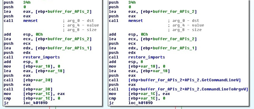
Figure 4.40 – Mapping a local variable to the corresponding structure field

Make sure that the Check operand option is enabled when renaming the operand to verify that the total sum of values remains accurate.

Another option is to select the text of the variable (not just left-click on it), right-click the Structure offset option (again, the T hotkey), specify the offset delta value, which should be equal to the offset of the pointer at the beginning of the structure, and finally select the structure field that’s suggested.

This method is quicker but doesn’t preserve the name of the pointer, as shown in the following screenshot:

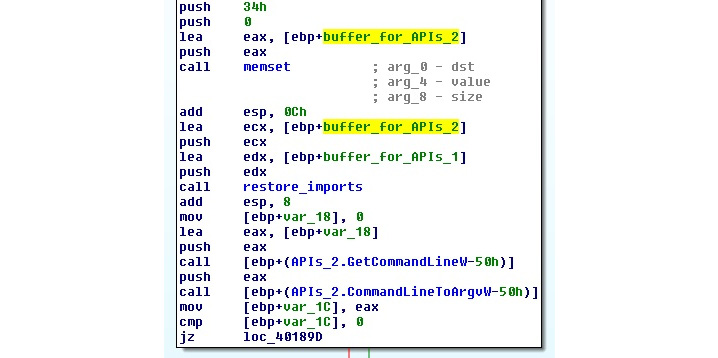
Figure 4.41 – Another way to map a local variable to the structure field

• Many custom encryption algorithms incorporate the xor operation, so the easy way to find them is by following these steps:
  1. Open the Text search window (the Alt + T hotkey).
  2. Type xor in the String field and search for it.
  3. Check the Find all occurrences checkbox.
  4. Sort the results and search for xor instructions that incorporate two different registers or a value in memory that is not accessed using the frame pointer register (ebp).
• Don’t hesitate to use free plugins such as FindCrypt, IDAscope, or IDA Signsrch that can search for encryption algorithms by signatures. Another great alternative to them is a standalone tool called capa, where you can use the –v command-line argument to get the virtual addresses of identified functions.
• If you need to import a C file with a list of definitions as enums, it is recommended that you use the h2enum.idc script (don’t forget to provide a correct mask in the second dialog window). When importing C files with structures, it generally makes sense to prepend them with a #pragma pack(1) statement to keep offsets correct. Both the File | Load file | Parse C header file... option and the Tilib tool can be used pretty much interchangeably.
• If you need to rename multiple consequent values that are pointing to the actual APIs in the populated import table, select all of them and execute the renimp.idc script, which can be found in IDA’s idc directory.
• If you need to have both IDA <= 6.95 and IDA 7.0+ together on one Windows machine, do the following:
  1. Install both x86 and x64 Python to different locations – for example, C:Python27 and C:Python27x64.
  2. Make sure that the following environment variables point to the setup for IDA <= 6.95:

  set PYTHONPATH=C:Python27;C:Python27Lib;C:Python27DLLs;C:Python27Liblib-tk;

  set NLSPATH=C:IDA6.95

By doing this, IDA <= 6.95 can be used as usual by clicking on its icon. To execute IDA 7.0+, create a special LNK file that will redefine these environment variables before executing IDA:

C:WindowsSystem32cmd.exe /c “SET PYTHONPATH=C:Python27x64;C:Python27x64Lib;C:Python27x64DLLs;C:Python27x64Liblib-tk; && SET NLSPATH=C:IDA7.0 && START /D ^”C:IDA7.0^” ida.exe”

• If your IDA version is shipped without FLIRT signatures for the Delphi programming language, it is still possible to mark them using an IDC script generated by the IDR tool. It is recommended to apply only names from the scripts that it produces.
• Recent versions of IDA provide decent support for the programs written in the Go language. For older versions of IDA, you should use plugins such as golang_loader_assist and IDAGolangHelper.
• To handle variable extension obfuscation, if the IDA Hex-Rays decompiler is available, use the D-810 plugin based on the Z3 project. Here is what its interface looks like:

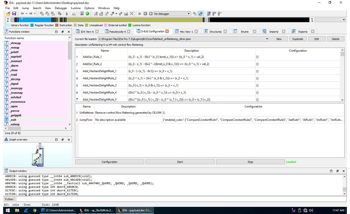
Figure 4.42 – Deobfuscation rules supported by the D-810 plugin

• Often, malware samples come with open source libraries such as OpenSSL that are statically linked to take advantage of the properly implemented encryption algorithms. Analyzing such code can be quite tricky, as it may not be immediately obvious which part of the code belongs to malware and which part belongs to the legitimate library. In addition, it may take a reasonable amount of time to figure out the purpose of each function within the library itself. Open source projects such as FLIRTDB and sig-database provide FLIRT signatures for the OpenSSL library for many operating systems. In addition, it is possible to create FLIRT signatures that can be reused later for other samples. Here’s how you can do this; we will be using OpenSSL as an example:
  1. Either find the already compiled file or compile a .lib/.a file for OpenSSL for the required platform (in our case, this is Windows). The compiler should be as close to the one that was used by the malware as possible.
  2. Get Flair utilities for your IDA from the official website. This package contains a set of tools for generating unified PAT files from various object and library formats (OMF, COFF, and so on), as well as the sigmake tool.
  3. Generate PAT files, for example, by using the pcf tool:

  pcf libcrypto.a libcrypto.pat

4. Use sigmake to generate .sig files:

sigmake libcrypto.pat libcrypto.sig

If necessary, resolve collisions by editing the .exc file that was created and rerun sigmake.

5. Place the resulting .sig file in the sig folder of the IDA root directory.
6. Follow these steps to learn how to use it:
   1. Go to View | Open subviews | Signatures (the Shift + F5 hotkey).
   2. Right-click Apply new signature (the Ins hotkey).
   3. Find the signature with the name you specified and confirm it by pressing OK or double-clicking on it.
   4. Another way to do this is by using the File | Load file | FLIRT signature file... option.

Another popular option for creating custom FLIRT signatures is the idb2pat tool.

Now, let’s talk about IDA capabilities in terms of dynamic analysis.

Dynamic analysis

These days, apart from its classic disassembler capabilities, IDA features multiple debugging options. Here are some tips and tricks that aim to facilitate dynamic analysis in IDA:

• To debug samples in IDA, make sure that the sample has an executable file extension (for example, .exe); otherwise, older versions of IDA may refuse to execute it, saying that the file does not exist.
• Older versions of IDA don’t have the Local Windows debugger option available for x64 samples. However, it is possible to use the Remote Windows debugger option together with the win64_remotex64.exe server application located in the IDA’s dbgsrv folder. It is possible to run it on the same machine if necessary and make them interact with each other via localhost using the Debugger | Process options... option.

The graph view only shows graphs for recognized or created functions. It is possible to quickly switch between text and graph views using the spacebar hotkey. When debugging starts, the Graph overview window in the graph view may disappear, but it can be restored by selecting the View | Graph Overview option.

• By default, IDA runs an automatic analysis when it opens the file, which means that any code that’s unpacked later won’t be analyzed. To fix this dynamically, follow these steps:
  1. If necessary, make the IDA recognize the entry point of the unpacked block as code by pressing the C hotkey. Usually, it also makes sense to make a function from it using the P hotkey.
  2. Mark the memory segment that stores the unpacked code as a loader segment. Follow these steps to do this:
     1. Go to View | Open subviews | Segments (the Shift + F7 hotkey combination).
     2. Find the segment storing the code of interest.
     3. Either right-click on it and select the Edit segment... option or use the Ctrl + E hotkey combination.
     4. Put a tick in the Loader segment checkbox.
  3. Rerun the analysis by either going to Options | General... | Analysis and pressing the Reanalyze program button or right-clicking in the bottom-left corner of the main IDA window and selecting the Reanalyze program option there.
• If you need to unpack a DLL, follow these steps:
  1. Load it into IDA just like any other executable.
  2. Choose your debugger of preference:
     • Local Win32 debugger for 32-bit Windows
     • Remote Windows debugger with the win64_remote64.exe application for 64-bit Windows
  3. Go to Debugger | Process options..., where you should do the following:
  • Set the full path of rundll32.exe (or regsvr32.exe for COM DLL, which can be recognized by DllRegisterServer/DllUnregisterServer or the DllInstall exports that are present) to the Application field.
  • Set the full path to the DLL in the Parameters field. Additional parameters will vary, depending on the type of DLL:

a. For a typical DLL that’s loaded using rundll32.exe, append either a name or a hash followed by the ordinal (for example, #1) of the export function you want to debug and separate it from the path by a comma. You have to provide an argument, even if you want to execute only the main entry point logic.

b. For Control Panel (CPL) DLLs that can be recognized by the CPlApplet export, the shell32.dll,Control_RunDLL argument can be specified before the path to the analyzed DLL instead.

c. For the COM DLLs that are generally loaded with the help of regsvr32.exe, the full path should be prepended with the /u argument in case the DllUnregisterServer export needs to be debugged. For a DllInstall export, a combination of /n/i[:cmdline] arguments should be used instead.

d. If the DLL is a service DLL (generally, it can be recognized by the ServiceMain export function and services-related imports) and you need to properly debug ServiceMain, see Chapter 3, Basic Static and Dynamic Analysis for x86/x64, for more details on how to debug services.

• Among other scripts that are useful for dynamic analysis, the funcap tool appears to be extremely handy as it allows you to record arguments that have been passed to functions during the execution process and keep them in comments once it’s done.
• If, after decryption, the malware constantly uses code and data from another memory segment (Trickbot is a good example), it is possible to dump these segments and then add them separately to the IDB using the File | Load File | Additional binary file... option. When using it, it makes sense to set the Loading segment value to 0 and specify the actual virtual address in the Loading offset field. If the engineer has already put the virtual address value (in paragraphs) in the Loading segment area and kept the loading offset equal to 0 instead, it is possible to fix it by going to View | Open subviews | Selectors and changing the value of the associated selector to zero.

Classic and new syntax of IDA scripts

Talking about scripting, the original way to write IDA scripts was to use a proprietary IDC language. It provides multiple high-level APIs that can be used in both static and dynamic analysis. Later, IDA started supporting Python and providing access to IDC functions with the same names under the idc module. Another functionality (generally, this is more low level) is available in the idaapi and idautils modules, but for automating most generic things, the idc module is good enough.

Since the list of APIs has extended over time, more and more naming inconsistencies have been accumulated. Eventually, at some stage, it started requiring a revision, which would be impossible to implement while keeping it backward-compatible. As a result, starting from IDA version 7.0 (the next version after 6.95), a new list of APIs was introduced that affected plugins that relied on the SDK and IDC functions. Some of them were just renamed from CamelCase to underscore_case, while others were replaced with new ones.

Here are some examples of them, showing both the original and new syntax:

• Navigation:
  • Functions/NextFunction: get_next_func allows you to iterate through functions.
  • Heads/NextHead: next_head allows you to iterate through instructions.
  • ScreenEA: get_screen_ea gets a sample’s virtual address where the cursor is currently located.
• Data access:
  • Byte/Word/Dword: byte/word/dword reads a value of a particular size.
• Data modification:
  • PatchByte/PatchWord/PatchDword: patch_byte/patch_word/patch_dword writes a block of a particular size.
  • OpEnumEx: op_enum converts an operand into an enum value.

Auxiliary data storage:

• AddEnum: add_enum adds a new enum.
• AddStrucEx: add_struc adds a new structure.

Here is an example of an IDA Python script implementing a custom XOR decryption algorithm for short blocks:

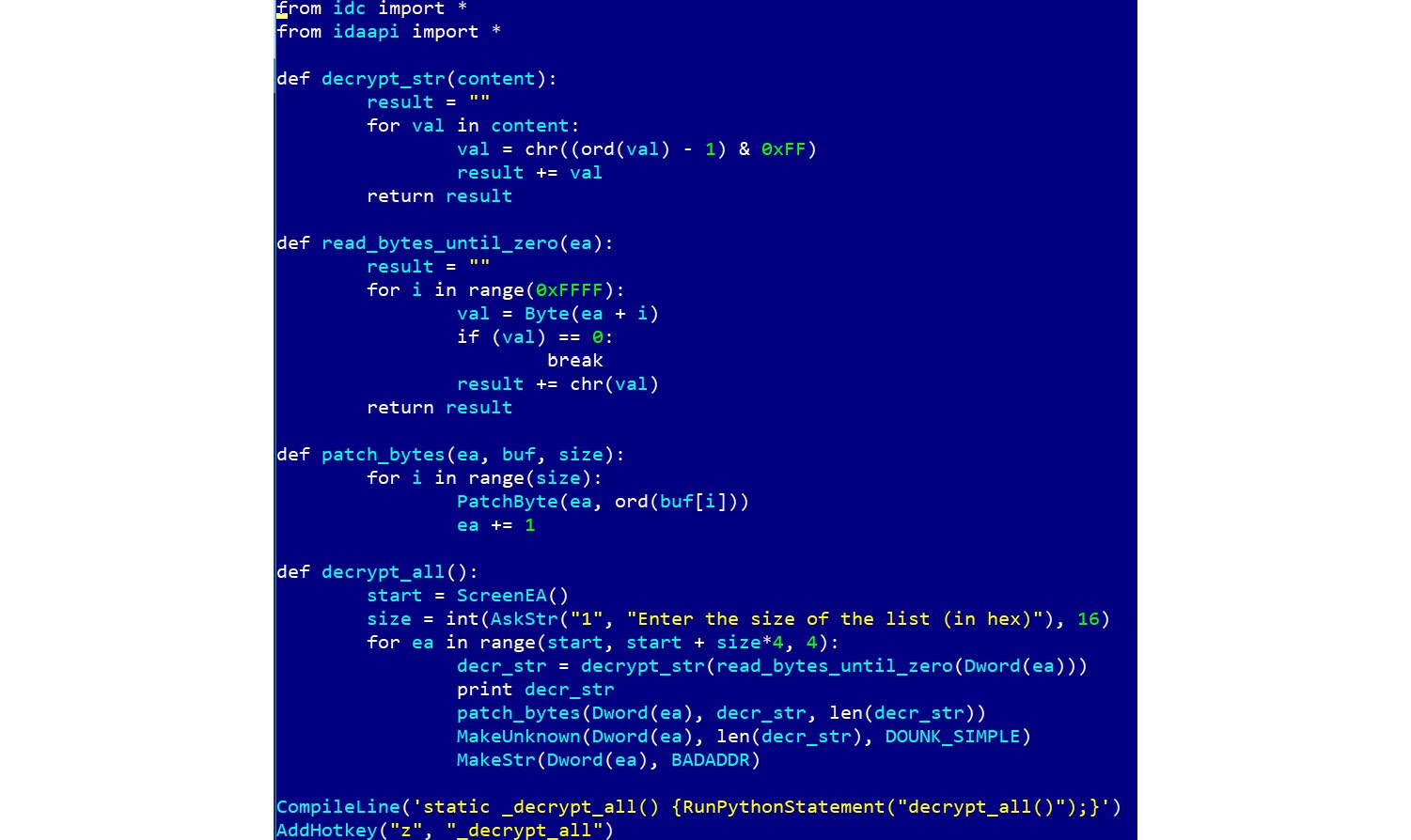
Figure 4.43 – Original IDA Python API syntax for 32-bit Windows

Here is a script implementing the same custom XOR decryption algorithm for a 64-bit architecture using the new syntax:

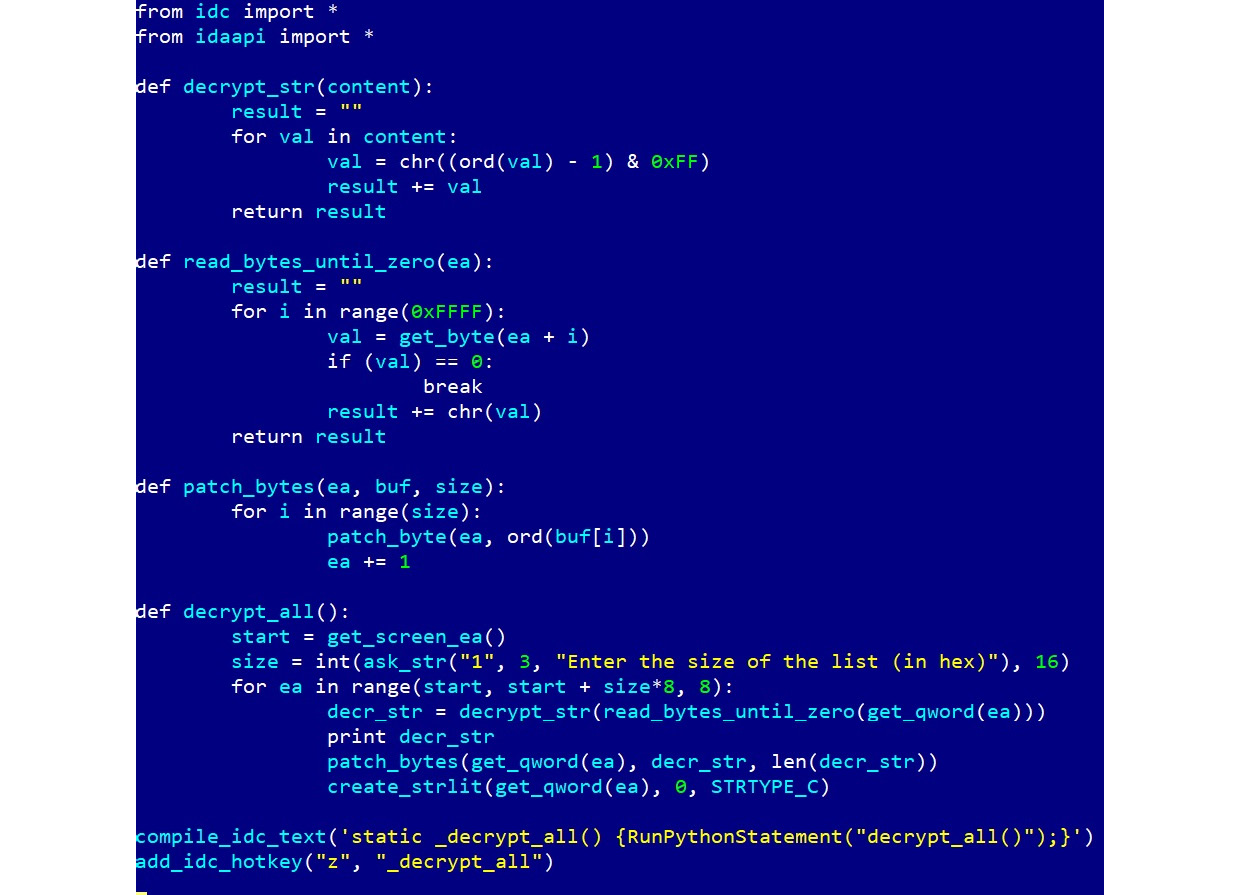
Figure 4.44 – New IDA Python API syntax for 64-bit Windows

Some situations may require an enormous amount of time to analyze a relatively big sample (or several of them) if the engineer doesn’t use IDA scripting and malware is using dynamic string decryption and dynamic WinAPIs resolution.

Dynamic string decryption

In this case, the block of encrypted strings is not decrypted at once. Instead, each string is decrypted immediately before being used, so they are never decrypted all at the same time. To solve this problem, follow these steps:

1. Find a function that’s responsible for decrypting all strings.
2. Replicate the decryptor’s behavior in a script.
3. Let the script find all the places in the code where this function is being called by following cross-references and read an encrypted string that will be passed as its argument.
4. Decrypt it and write it back on top of the encrypted one so that all the references will remain valid.

Dynamic WinAPIs resolution

With the dynamic WinAPIs resolution, only one function with different arguments is used to get access to all the WinAPIs. It dynamically searches for the requested API (and often the corresponding DLL), usually using some sort of checksum of the name that’s provided as an argument. There are two common approaches to making this readable:

• Using enums:
  1. Find the matches between all checksums, APIs, and DLLs used.
  2. Store the associations as enum values.
  3. Find all the places where the resolving function is being used, take its checksum argument, and convert it into the corresponding enum name.
• Using comments:
  1. Find the matches between all checksums, APIs, and DLLs used.
  2. Store the associations in memory.
  3. Find all the places where the resolving function is being used, take its checksum argument, and place a comment with the corresponding API name next to it.

IDA scripting is really what makes a difference and turns novice analysts into professionals who can efficiently solve any reverse engineering problem promptly. After you have written a few scripts using this approach, it becomes pretty straightforward to update or extend them with extra functionality for new tasks.

Summary

In this chapter, we covered various types of packers and explained the differences between them. We also gave recommendations on how we can identify the packer that’s being used. Then, we went through several techniques of how to unpack samples both automatically and manually and provided real-world examples of how to do so in the most efficient way, depending on the context. After this, we covered advanced manual unpacking methods that generally take more time to execute but give you the ability to unpack virtually any sample in a meaningful time frame.

Furthermore, we covered different encryption algorithms and provided guidelines on how to identify and handle them. Then, we went through a modern malware example that incorporated these guidelines so that you could get an idea of how all this theory can be applied in practice. Finally, we covered IDA script languages – a powerful way to drastically speed up the analysis process.

In Chapter 5, Inspecting Process Injection and API Hooking, we are going to expand our knowledge about various techniques that are used by malware authors to achieve their goals and provide a handful of tips on how to deal with them.