2

A Crash Course in Assembly and Programming Basics

Before diving deeper into the malware world, we need to have a complete understanding of the core of the machines we are analyzing malware on. For reverse engineering purposes, it makes sense to focus largely on the architecture and the operating system (OS) it supports. Of course, multiple devices and modules comprise a system, but it is mainly these two that define a set of tools and approaches that are used during the analysis. The physical representation of any architecture is a processor. A processor is like the heart of any smart device or computer in that it keeps it alive.

In this chapter, we will cover the basics of the most widely used architectures, from the well-known x86 and x64 Instruction Set Architectures (ISAs) to solutions that power multiple mobile and Internet of Things (IoT) devices, which are often misused by malware families, such as Mirai. This will set the tone for your journey into malware analysis, as static analysis is impossible without understanding assembly instructions. Although modern decompilers are becoming better and better, they don’t exist for all platforms that are targeted by malware. Besides, they will probably never be able to handle obfuscated code. Don’t be daunted by the complexity of assembly; it just takes time to get used to it, and after a while, it becomes possible to read it like any other programming language. While this chapter provides a starting point, it always makes sense to deepen your knowledge by practicing and exploring further.

In this chapter, we will cover the following topics:

• Basics of informatics
• Architectures and their assembly
• Becoming familiar with x86 (IA-32 and x64)
• Exploring ARM assembly
• Basics of MIPS
• Covering the SuperH assembly
• Working with SPARC
• Moving from assembly to high-level programming languages

Basics of informatics

Before we dive deeper into the internals of the various architectures, now is a good time to revise the numeral systems, which will lay a foundation for understanding both data types and bitwise operations.

Numeral systems

In our daily life, we use the decimal system with digits from 0 to 9, which gives us 10 different 1-digit options in total. There is a good reason for that – most of us as human beings have 10 fingers on our hands in total, which are always in front of us and are great tools for counting. However, from a data science point of view, there is nothing particular about the number 10. Using another base would allow us to store information much more efficiently.

The absolute minimum required to store some information is two different values: yes or no, true or false, and so on. This lays a foundation for the binary numeral system that uses only two digits: 0 and 1. The way we use it is the same as in the case of decimal: every time we reach the maximum digit on the right, we drop it to 0 and increment the next digit to the left from it while following the same logic. Therefore, 0, 1, 2, 3, 4, ... 9, 10, 11, ... becomes 0, 1, 10, 11, 100, ..., 1001, 1010, 1011, ... and so on. This approach makes it possible to efficiently encode big amounts of information to be read automatically by machines. Examples include magnetic tapes and floppy disks (lack or presence of magnetization), CD/DVD/BD (lack or presence of the indentation read by a laser), and flash memory (lack or presence of the electric charge). To not mix up binary values with decimals, it is common to use the “b” suffix for binary values (for example, 1010b).

Now, if we want to work with groups of binary digits, we need to choose the size of the group. The group of 3 (from 000 to 111) would give 2^3 = 8 possible combinations of 0 and 1, allowing us to encode eight different numbers. Similarly, the group of 4 (from 0000 to 1111) would give 2^4 = 16 possible combinations. This is why octal and hexadecimal systems started to be used: they allow you to efficiently convert binary numbers. The octal system uses the base of 8, which means it can use digits from 0 to 7. The hexadecimal system supports 16 digits, which were encoded using digits 0 to 9, followed by the first six letters of the English alphabet: A to F. Here, hexadecimal A stands for decimal 10, B stands for 11, and so on up to the maximum possible value of F, which stands for decimal 15. The way we use them is the same as for decimal and binary numeral systems: once the maximum digit on the right is reached, the next value would have dropped back to 0 and the digit to the left from it incremented while following the same logic. In this case, a decimal sequence such as 14, 15, 16, 17 will be represented as E, F, 10, 11 in hexadecimal. To not confuse hexadecimal numbers with decimals, you can use the “0x” and “x” prefixes or the “h” suffix to mark hexadecimal numbers (for example, 0x33, x73, and 70h).

Converting binary values into hexadecimal is extremely easy. The whole binary value should be split into groups of four digits, where each group will represent a single hexadecimal digit. For example, 0001b = 1h and 00110001b comprising 0011b = 3h and 0001b = 1h gives us 31h.

Now, it is time to learn how different data types are encoded using this approach.

Basic data units and data types

As we know, the smallest data storage unit should be able to store two different values – a 0 or a 1; that is, a single digit in the binary numeral system. This unit is called a bit. A group of 8 bits comprises a byte. A single byte can be used to encode all possible combinations of zeroes and ones from 00000000b to 11111111b, which gives us 2^8 = 256 different variants in total, from 0x0 to 0xFF. Other widely used data units are word (2 bytes), dword (4 bytes), and qword (8 bytes).

Now, let’s talk about how we can encode the data that’s stored using these data units. Here are some of the most common primitive data types found in various programming languages:

• Boolean: A binary data type that can only store two possible values: true or false.
• Integer: This stores whole numbers. The size varies. In some cases, it can be specified as a suffix defining the number of bits (int16, int32, and so on).
• Unsigned: All bits are dedicated to storing the numeric value.
• Signed: The most significant bit (the top left) is dedicated to storing the sign, 0 for plus and 1 for minus. So 0xFFFFFFFF = -1.
• Short and long: These data types are integers that are smaller or bigger than the standard integer, respectively. The size is 2 bytes for short and 4 or 8 bytes for long.
• Float and double: These data types are designed to store floating-point numbers (values that can have fractions). They are pretty much never used in malware.
• Char: Generally used to store characters of strings, each value has a size of 1 byte.
• String: A group of bytes that defines human-readable strings. It can utilize one or multiple bytes per character, depending on the encoding.
• ASCII: Defines the mappings between characters (letters, numbers, punctuation signs, and so on) and the byte values. It uses 7 bits per character:
  

Figure 2.1 – ASCII table

Figure 2.1 – ASCII table

• Extended ASCII: Utilizes 8 bits per character, where the first half (0x0-0x7F) is equal to the ASCII table and the rest depend on the code page (for example, Windows-1252 encoding).
• UTF8: This is a Unicode encoding that uses 1 to 4 bytes per character. It’s commonly used in the *nix world. The beginning matches the ASCII table.
• UTF16: This is a Unicode encoding that uses 2 or 4 bytes per character. The order of the bytes depends on the endianness.
• Little Endian: The least significant byte goes to the lowest address (UTF16-LE, the default Unicode encoding used by the Windows OS; the corresponding strings are known as Wide strings there).
• Big Endian: The most significant byte goes to the lowest address (UTF16-BE):

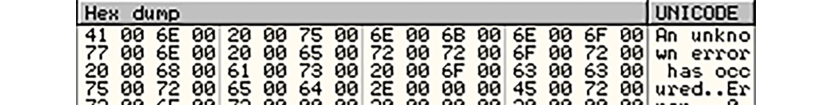
Figure 2.2 – Example of a UTF16-LE string

Apart from knowing how the data can be stored using bits, it is also important to understand bitwise operations as they have multiple applications in assembly.

Bitwise operations

Bitwise operations operate at the bit level and can be unary, which means they only require one operand, and binary, which means they work with two operands and apply the corresponding logic to each pair of the aligned bits. Because they are fast to perform, bitwise operations have found multiple applications in machine code. Let’s look at the most important ones.

AND (&)

Here, the result bit will only be set (become equal to 1) if both corresponding operand bits are equal to 1.

The following is an example:

10110111b

AND

11001001b

=

10000001b

The most common application of this operation in assembly is to separate part of the provided hexadecimal value (operand #1) by using a mask (operand #2) and nullify the rest. It is based on two features of this operation:

• If one operand’s bit is set to 0, the result will always be 0
• If one operand’s bit is set to 1, the result will be equal to another operand’s bit

Therefore, 0x12345678 & 0x000000FF = 0x00000078 (as 0xFF = 11111111b).

OR (|)

In this case, the result bit will be equal to 1 if any of the corresponding operand bits are equal to 1.

The following is an example:

10100101b

OR

10001001b

=

10101101b

Here, the common application of this operation is setting bits by mask while preserving the rest of the value. It is based on the following features of this operation:

• If one operand’s bit is set to 0, the result will be equal to another operand’s bit
• If one operand’s bit is set to 1, the result will always be 1

This way, 0x12345678 & 0x000000FF = 0x123456FF (again, as 0xFF = 11111111b).

XOR (^)

Here, the result bit will only be 1 if the corresponding operands’ bits are different. Otherwise, the result is 0.

The following is an example:

11101001b

XOR

10011100b

=

01110101b

There are two very common applications of this operation:

• Nullification: This is based on the principle that if we use the same value for both operands, all its bits will meet equal bits, so the whole result will be 0.
• Encryption: This is based on the fact that applying this operation twice with the same key as one of the operands restores the original value. The actual property it is based on is that if one of the operands is 0, the result will be equal to another operand, and this is exactly what happens in the end:
  • plain_text ^ key = encrypted_text
  • encrypted_text ^ key = (plain_text ^ key) ^ key = plain_text ^ (key ^ key) = plain_text ^ 0 = plain_text

Now let’s look at the NOT (~) operation.

NOT (~)

Unlike the previous operations, this operation is unary and requires only one operand, flipping all its bits to the opposite ones.

The following is an example:

NOT

11001010b

=

00110101b

The common application of this operation is to change the sign of signed integer values to the opposite one (for example, -3 to 3 or 5 to -5). The formula, in this case, will be ~value + 1.

Now, let’s take a look at bit shifts.

Logical shift (<< or >>)

This operation requires the direction (left or right) to be specified, along with the actual value to change and the number of shift positions. During the shift, each bit of the original value will move to the left or right on the number of positions specified; the empty spaces on the opposite side are filled in with zeroes. All bits shifted outside of the data unit are lost.

The following are some examples:

10010011b >> 1 = 01001001b

10010011b << 2 = 01001100b

There are two common applications of this operation:

• Moving the data to a particular part of the register (as you’ll see shortly)
• Multiplication (shift left) or division (shift right) by a power of two for every shift position

Circular shift (Rotate)

This bitwise shift is very similar to the logical shift with one important difference – all the bits shifted out on one side of the data unit will appear on the opposite side.

The following are some examples:

10010011b ROR 1 = 11001001b

10010011b ROL 2 = 01001110b

Because, unlike logical shift, the operation is reversible and the data is not lost, it can be used in cryptography algorithms.

Other types of shifts, such as arithmetic shift or rotate with carrying, are present much more rarely in the assembly in general and in malware in particular, so they are outside the scope of this book.

Now, it is finally time to start learning more about various architectures and their assembly instructions.

Architectures and their assembly

Simply put, the processor, also known as the central processing unit (CPU), is quite similar to a calculator. If you look at the instructions (whatever the assembly language is), you will find many of them dealing with numbers and doing some calculations. However, multiple features differentiate processors from usual calculators. Let’s look at some examples:

• Modern processors support a much bigger memory space compared to traditional calculators. This memory space allows them to store billions of values, which makes it possible to perform more complex operations. Additionally, they have multiple fast and small memory storage units embedded inside the processors’ chips called registers.
• Processors support many instruction types other than arithmetic instructions, such as changing the execution flow based on certain conditions.
• Processors can work in conjunction with other peripheral devices such as speakers, microphones, hard disks, graphics cards, and others.

Armed with such features and coupled with great flexibility, processors became the go-to universal machines to power various advanced modern technologies such as machine learning. In the following sections, we will explore these features before diving deeper into different assembly languages and how these features are manifested in these languages’ instruction sets.

Registers

Even though processors have access to a huge memory space that can store billions of values, this storage is provided by separate RAM devices, which makes it longer for the processors to access the data. So, to speed up the processor operations, they contain small and fast internal memory storage units called registers.

Registers are built into the processor chip and can store the immediate values that are needed while performing calculations and data transfers from one place to another.

Registers may have different names, sizes, and functions, depending on the architecture. Here are some of the types that are widely used:

• General-purpose registers: These are registers that are used to temporarily store arguments and results for various arithmetic, bitwise, and data transfer operations.
• Stack and frame pointers: These point to the top and a certain fixed point of the stack (as you’ll see shortly).
• Instruction pointer/program counter: The instruction pointer is used to point to the next instruction to be executed by the processor.

Memory

Memory plays an important role in the development of all the smart devices that we use nowadays. The ability to manage lots of values, text, images, and videos on a fast and volatile memory allows CPUs to process more information and, eventually, perform more complicated operations, such as displaying graphical interfaces in 3D and virtual reality.

Virtual memory

In modern OSs, whether they are 32-bit or 64-bit based, the OS creates an isolated virtual memory (in which its pages are mapped to the physical memory pages) for each process. Applications are only supposed to have the ability to access their virtual memory. They can read and write code and data and execute instructions located in virtual memory. Each memory range that comprises virtual memory pages has a set of permissions, also known as protection flags, assigned to it, which represents the types of operations the application is allowed to perform on it. Some of the most important of them are READ, WRITE, and EXECUTE, as well as their combinations.

For an application to attempt to access a value stored in memory, it needs its virtual address. Behind the scenes, the Memory Management Unit (MMU) and the OS are transparently mapping these virtual addresses to physical addresses that define where the values are stored in hardware:

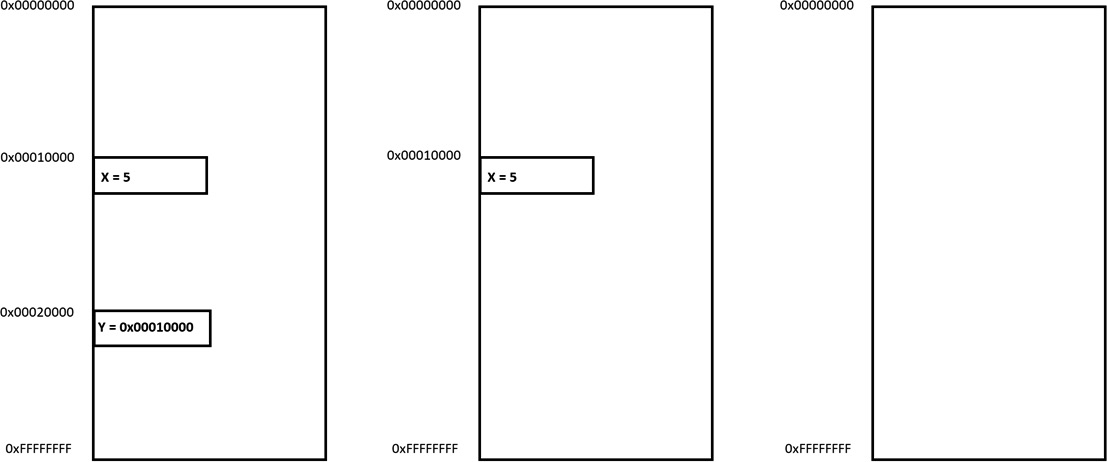
Figure 2.3 – Virtual memory addresses

To save the space that’s required to store and use addresses of values, the concept of the stack has been developed.

Stack

A stack is a pile of objects. In computer science, the stack is a data structure that helps save different values of the same size in memory in a pile structure using the principle of Last In First Out (LIFO).

The top of the stack (where the next element will be placed) is pointed to by a dedicated stack pointer, which will be discussed in greater detail shortly.

A stack is common among many assembly languages and it may serve multiple purposes. For example, it may help in solving mathematical equations, such as X = 5*6 + 6*2 + 7(4 + 6), by temporarily storing each calculated value and later pulling them back to calculate the sum of all of them and saving them in a variable, X.

Another application for the stack is to pass arguments to functions and store local variables. Finally, on some architectures, a stack can also be used to save the address of the next instruction before calling a function. This way, once this function finishes executing, it is possible to pop this return address back from the top of the stack and transfer control to where it was called from to continue the execution.

While the stack pointer is always pointing to the current top of the stack, the frame pointer is storing the address of the top of the stack at the beginning of the function to make it possible to access passed arguments and local variables, and also restore the stack pointer value at the end of the routine. We will cover this in greater detail when we talk about calling conventions for different architectures.

Instructions (CISC and RISC)

Instructions are machine code represented in the form of bytes that CPUs can understand and execute. For us humans, reading bytes is extremely problematic, which is why we developed assemblers to convert assembly code into instructions and disassemblers to be able to read it back.

Two big groups of architectures define assembly languages that we will cover in this section: Complex Instruction Set Computer (CISC) and Reduced Instruction Set Computer (RISC).

Without going into too many details, the main difference between CISC assemblies, such as Intel IA-32 and x64, and RISC assembly languages associated with architectures such as ARM is the complexity of their instructions.

CISC assembly languages have more complex instructions. They generally focus on completing tasks using as few lines of assembly instructions as possible. To do that, CISC assembly languages include instructions that can perform multiple operations, such as mul in Intel assembly, which performs data access, multiplication, and data store operations in one go.

In the RISC assembly language, assembly instructions are simple and generally perform only one operation each. This may lead to more lines of code to complete a specific task. However, it may also be more efficient, as this omits the execution of any unnecessary operations.

Overall, we can split all the instructions, regardless of the architecture, into several groups:

• Data manipulation: This comprises arithmetic and bitwise operations.
• Data transfer: Allows data that may involve registers, memory, and immediate values to be moved.
• Control flow: This makes it possible to change the order the instructions are executed in. In every assembly language, there are multiple comparison and control flow instructions, which can be divided into the following categories:
  • Unconditional: This type of instruction forcefully changes the flow of the execution to another address (without any given condition).
  • Conditional: This is like a logical gate that switches to another branch based on a given condition (such as equal to zero, greater than, or less than), as shown in the following diagram:

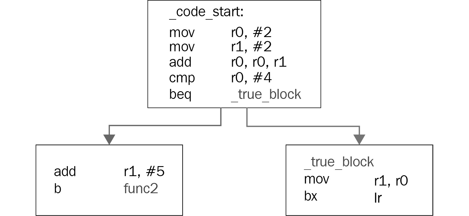
Figure 2.4 – An example of a conditional jump

• Subroutine call: These instructions change the execution to another function and save the return address to be restored later when necessary.

Now, it is time to learn about the most common instructions that you may see when performing reverse engineering. Becoming able to read them fluently and understand the meaning of groups of them is an important step in the journey of becoming a professional malware analyst.

Becoming familiar with x86 (IA-32 and x64)

Intel x86 (including both 32 and 64-bit versions) is the most common architecture used in PCs. It powers various types of workstations and servers, so it comes as no surprise that most of the malware samples we have at the moment support it. The 32-bit version of it, IA-32, is also commonly referred to as i386 (succeeded by i686) or even simply x86, while the 64-bit version, x64, is also known as x86-64 or AMD64. x86 is a CISC architecture, and it includes multiple complex instructions in addition to simple ones. In this section, we will introduce the most common of them and cover how the functions are organized.

Registers

The following table shows the relationship between the registers in the IA-32 and x64 architectures:

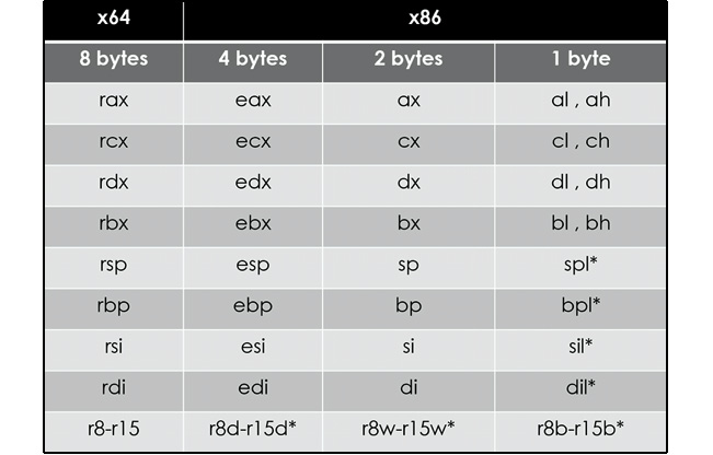
Figure 2.5 – IA-32 and x64 architectures

The registers that are used in the x86 architectures (the 8 to r15 registers) are only available in x64, not IA-32, and the spl, bpl, sil, and dil registers can only be accessed in x64.

The first thing to mention is that there may be multiple interpretations of what registers should be called general-purpose registers (GPRs) and which are not since most of them may serve some particular purpose.

The first four registers (rax/eax, rbx/ebx, rcx/ecx, and rdx/edx) are GPRs. Some of them have special use cases for certain instructions:

• rax/eax: This is commonly used to store the result of some operations and the return values of functions.
• rcx/ecx: This is used as a counter register in instructions that’s responsible for repeating actions.
• rdx/edx: This is used in multiplication and division to extend the result or the dividend, respectively.

In x64, the registers from r8 to r15 were added to the list of available GPRs.

rsi/esi and rdi/edi are mostly used to define addresses when copying groups of bytes in memory. The rsi/esi register always plays the role of the source, while the rdi/edi register plays the role of the destination. Both registers are non-volatile and are also GPRs.

The rsp/esp register is used as a stack pointer, which means it always points to the top of the stack. Its value decreases when a value is getting pushed to the stack, and increases when a value is getting pulled out from the stack.

The rbp/ebp register is mainly used as a base pointer that indicates a fixed place within the stack. It helps access the function’s local variables and arguments, as we will see later in this section.

Special registers

There are two special registers in the x86 assembly, as follows:

• rip/eip: This is an instruction pointer that points to the next instruction to be executed. It cannot be accessed directly but there are special instructions that work with it.
• rflags/eflags/flags: This register contains the current state of the processor. Its flags are affected by the arithmetic and logical instructions, including comparison instructions such as cmp and test, and it’s used with conditional jumps and other instructions as well. Here are some of its flags:
  • Carry flag (CF): This flag is set when an arithmetic operation goes out of bounds, as follows:

mov al, FFh ; al = 0xFF & CF = 0

add al, 1 ; al = 0 & CF = 1

• Zero flag (ZF): This flag is set when the arithmetic or a logical operation’s result is zero. This can also be set by comparison instructions.
• Direction flag (DF): This indicates whether certain instructions such as lods, stos, scas, and movs (as you’ll see shortly) should go to higher addresses (when not set) or to lower addresses (when set).
• Sign flag (SF): This flag indicates that the result of the operation is negative.
• Overflow flag (OF): This flag indicates that an overflow occurred in an operation, leading to a change in the sign (only for signed numbers), as follows:

mov cl, 7Fh ; cl = 0x7F (127) & OF = 0

inc cl ; cl = 0x80 (-128) & OF = 1

There are other registers as well, such as the MMX and FPU registers (and instructions to work with them), but they are rarely used in malware, so they are outside the scope of this book.

The instruction structure

Many x86 assemblers, such as MASM and NASM, as well as disassemblers, use Intel syntax. In this case, the common structure of its instructions is opcode, dest, src.

dest and src are commonly referred to as operands. Their numbers can vary from 0 to 3, depending on the instruction. Another option would be GNU Assembler (GAS), which uses the AT&T syntax and swaps dest and src for representation. Throughout this book, we will use Intel syntax.

Now, let’s dive deeper into the meaning of each part of the instruction.

opcode

opcode is the name of the instruction that specifies the operation that was performed. Some instructions only have an opcode part without any dest or src, such as nop, pushad, popad, and movsb.

Important Note

pushad and popad are not available in x64.

dest

dest represents the destination, or where the result of the operation will be saved, and can also become part of the calculations themselves, like so:

add eax, ecx ; eax = (eax + ecx)

sub rdx, rcx ; rdx = (rdx - rcx)

dest could look as follows:

• REG: A register, such as eax or edx.
• r/m: A place in memory, such as the following:
  • DWORD PTR [00401000h]
  • BYTE PTR [EAX + 00401000h]
  • WORD PTR [EDX*4 + EAX+ 30]

The stack is also a place in memory:

• DWORD PTR [ESP+4]
• DWORD PTR [EBP-8]

src

src represents the source or another value in the calculations, but it is not used to save the results there afterward. It may look like this:

• REG: For instance, add rcx, r8
• r/m: For instance, add ecx, DWORD PTR [00401000h]
  • Here, we are adding the value of the size of DWORD located at the 00401000h address to ecx.
• imm: An immediate value, such as mov eax, 00100000h

For instructions with a single operand, it may play a role of both a source and a destination:

inc eax

dec ecx

Or, it could be only the source or the destination. This is the case for the following instructions, which save the value on the stack and then pull it back:

push rdx

pop rcx

The instruction set

In this section, we will cover the most important instructions required to start reading the assembly.

Data manipulation instructions

Some of the most common arithmetic instructions are as follows:

Important Note

For multiplication and division, which treat operands as signed integers, the corresponding instructions will be imul and idiv.

The following instructions represent logical/bitwise operations:

Lastly, the following instructions represent bitwise shifts and rotations:

To learn more about the potential applications of bitwise operations, please read Chapter 1, Cybercrime, APT Attacks, and Research Strategies.

Data transfer instructions

The most basic instruction for moving the data is mov, which copies a value from src to dest. This instruction has multiple forms, as shown in the following table:

Here are the instructions related to the stack:

Here are the string manipulation instructions:

Important Note

If the DF bit in the EFLAGS register is 0, these instructions will increase the value of the rdi/edi or rsi/esi register by the number of bytes used (1, 2, 4, or 8) and decrease if the DF bit is set (equals 1).

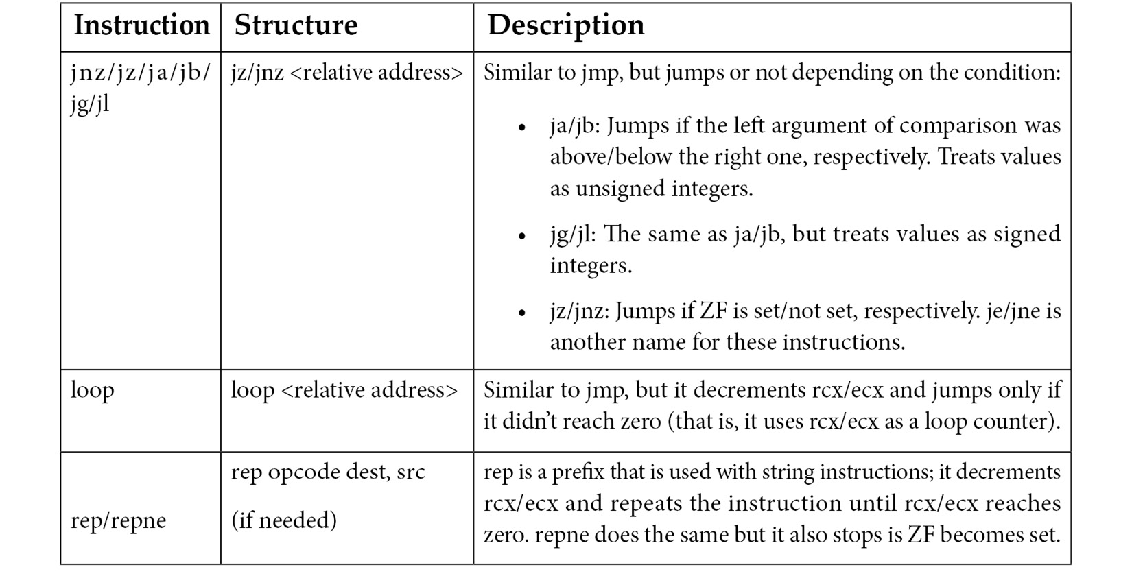
Control flow instructions

These instructions change the value of the rip/eip register so that the instructions to be executed next may not be the next ones sequentially. The most important unconditional redirections are as follows:

To implement the condition, some form of comparison needs to be used. There are dedicated instructions for that:

The following table shows some of the most important conditional redirections based on the result of this comparison:

Now, let’s talk about how values can be passed to functions and accessed there.

Arguments, local variables, and calling conventions (in x86 and x64)

Arguments can be passed to functions in various ways. These ways are called calling conventions. In this section, we will cover the most common ones. We will start with the standard call (stdcall) convention, which is commonly used in IA-32, and then cover the differences between it and other conventions.

stdcall

The stack, together with the rsp/esp and rbp/ebp registers, does most of the work when it comes to arguments and local variables. The call instruction saves the return address at the top of the stack before transferring the execution to the new function, while the ret instruction at the end of the function returns the execution to the caller function using the return address saved in the stack.

Arguments

In stdcall, the arguments are pushed in the stack from the last argument to the first (right to left), like this:

push Arg02 
push Arg01 
call Func01

In the Func01 function, the arguments could be accessed by esp, but it would be hard to always adjust the offset with every next value that’s pushed or pulled:

mov eax, [esp + 8] ; Arg01
push eax
mov ecx, [esp + C] ; Arg01 keeping in mind the previous push

Fortunately, modern static analysis tools, such as IDA Pro, can detect which argument is being accessed in each instruction, as in this case. However, the most common way to access arguments, as well as local variables, is by using ebp. First, the called function needs to save the current esp in the ebp register and then access it, like so:

push ebp
mov ebp, esp
...
mov ecx, [ebp + 8] ; Arg01
push eax
mov ecx, [ebp + 8] ; still Arg01 (no changes)

At the end of the called function, it returns the original values of ebp and esp, like this:

mov esp, ebp
pop ebp 
ret

As it’s a common function epilogue, Intel created a special instruction for it, called

leave, so it became as follows:

leave 
ret

Local variables

For local variables, the called function allocates space for them by decreasing the value of the esp register. To allocate space for two variables of four bytes each, use the following code:

push ebp
mov ebp, esp 
sub esp, 8

Again, the end of the function will look like this:

mov ebp, esp 
pop ebp 
ret

The following figure exemplifies how the stack change looks at the beginning and the end of the function:

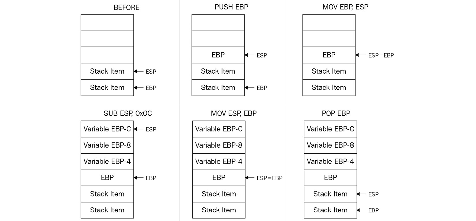
Figure 2.6 – An example of a stack change at the beginning and the end of the function

Additionally, if there are arguments, the ret instruction cleans the stack, given the number of bytes to pull out from the top of the stack, like this:

ret 8 ; 2 arguments, 4 bytes each

cdecl

cdecl (which stands for C declaration) is another calling convention that was used by many C compilers in x86. It’s very similar to stdcall, with the only difference being that the caller cleans the stack after the callee function (the called function) returns, like so:

Caller:
  push Arg02 
  push Arg01 
  call Callee
  add esp, 8 ; cleans up the stack

fastcall

The fastcall calling convention is also widely used by different compilers, including the Microsoft C++ compiler and GCC. This calling convention passes the first two arguments in ecx and edx and passes the remaining arguments through the stack. Again, it is only used in the 32-bit version of x86.

thiscall

For object-oriented programming and non-static member functions (such as the classes’ functions), the C compiler needs to pass the address of the object whose attribute will be accessed or manipulated using it as an argument.

In the GCC compiler, thiscall is almost identical to the cdecl calling convention and it passes the current object’s address (that is, this) as the first argument. But in the Microsoft C++ compiler, it’s similar to stdcall and passes the object’s address in ecx. It’s common to see such patterns in some object-oriented malware families.

Borland register

This convention can be commonly seen in malware written in the Delphi programming language. The first three arguments are passed through the eax, edx, and ecx registers while the rest go through the stack. However, unlike other conventions, they are passed in the opposite order – from left to right. If necessary, it will be the callee (called function) who cleans up the stack.

Microsoft x64 calling convention

In x64, the calling conventions are more dependent on the registers. For Windows, the caller function passes the first four arguments to the registers in the following order: rcx, rdx, r8, r9. The rest are passed through the stack. The calling function (caller) cleans the stack in the end (if necessary).

System V AMD64 ABI

For other 64-bit OSs such as Linux, FreeBSD, or macOS, the first six arguments are passed to the registers in this order: rdi, rsi, rdx, rcx, r8, r9. The remaining get passed through the stack. Again, it is the caller who cleans the stack in the end, if necessary. This is the only way to do this on 64-bit OSs.

Exploring ARM assembly

Most of you are probably more familiar with the x86 architecture, which implements the CISC design. So, you may be wondering, why do we need something else? The main advantage of RISC architectures is that the processors that implement them generally require fewer transistors, which eventually makes them more energy and heat-efficient and reduces the associated manufacturing costs, making them a better choice for portable devices. We have started our introduction to RISC architectures with ARM for a good reason – at the time of writing, this is the most widely used architecture in the world.

The explanation is simple – processors that implement it can be found on multiple mobile devices and appliances such as phones, video game consoles, or digital cameras, heavily outnumbering PCs. For this reason, multiple IoT malware families and mobile malware that target Android and iOS platforms have payloads for the ARM architecture; an example can be seen in the following screenshot:

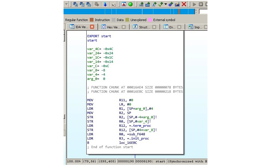
Figure 2.7 – Disassembled IoT malware targeting ARM-based devices

Thus, to analyze them, it is necessary to understand how ARM works.

ARM originally stood for Acorn RISC Machine, and later for Advanced RISC Machine. Acorn was a British company considered by many as the British Apple, producing some of the most powerful PCs of that time. It was later split into several independent entities, with Arm Holdings (currently owned by SoftBank Group) supporting and extending the current standard.

Multiple OSs support it, including Windows, Android, iOS, various Unix/Linux distributions, and many other lesser-known embedded OSs. The support for a 64-bit address space was added in 2011 with the release of the ARMv8 standard.

Overall, the following ARM architecture profiles are available:

• Application profiles (suffix A, for example, the Cortex-A family): These profiles implement a traditional ARM architecture and support a virtual memory system architecture based on am MMU. These profiles support both ARM and Thumb instruction sets (as discussed later).
• Real-time profiles (suffix R, for example, the Cortex-R family): These profiles implement a traditional ARM architecture and support a protected memory system architecture based on a Memory Protection Unit (MPU).
• Microcontroller profiles (suffix M, for example, the Cortex-M family): The profiles implement a programmers’ model and are designed to be integrated into Field Programmable Gate Arrays (FPGAs).

Each family has its corresponding set of associated architectures (for example, the Cortex-A 32-bit family incorporates the ARMv7-A and ARMv8-A architectures), which, in turn, incorporates several cores (for example, the ARMv7-R architecture incorporates Cortex-R4, Cortex-R5, and so on).

Basics

In this section, we will cover both the original 32-bit and the newer 64-bit architectures. Multiple versions were released over time, starting from the ARMv1. In this book, we will focus on the recent versions of them.

ARM is a load-store architecture; it divides all instructions into the following two categories:

• Memory access: Move data between memory and registers
• Arithmetic Logic Unit (ALU) operations: Do computations involving registers

ARM supports the addition, subtraction, and multiplication arithmetic operations, though some new versions, starting from ARMv7, also support division. It also supports big-endian order but uses little-endian order by default.

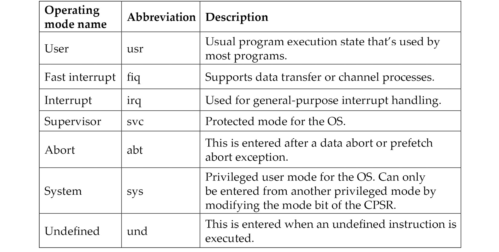
16 registers are visible at any time on the 32-bit ARM: R0-R15. This number is convenient as it only takes 4 bits to define which register is going to be used. Out of them, 13 (sometimes referred to as 14, including R14 or 15, also including R13) are general-purpose registers: R13 and R15 each have a special function, while R14 can take it occasionally. Let’s have a look at them in greater detail:

• R0-R7: Low registers are the same in all CPU modes.
• R8-R12: High registers are the same in all CPU modes except the Fast Interrupt Request (FIQ) mode, which is not accessible by 16-bit instructions.
• R13 (also known as SP): This is a stack pointer that points to the top of the stack. Each CPU mode has a version of it. It is discouraged to use it as a GPR.
• R14 (also known as LR): This is a link register. In user mode, it contains the return address for the current function, mainly when BL (Branch with Link) or BLX (Branch with Link and eXchange) instructions are executed. It can also be used as a GPR if the return address is stored on the stack. Each CPU mode has a version of it.
• R15 (also known as PC): This is a program counter that points to the currently executed command. It’s not a GPR.

Altogether, there are 30 general-purpose 32-bit registers on most of the ARM architectures overall, including the same name instances in different CPU modes.

Apart from these, there are several other important registers, as follows:

• Application Program Status Register (APSR): This stores copies of the ALU status flags, also known as condition code flags. On later architectures, it also holds the Q (saturation) and the greater than or equal to (GE) flags.
• Current Program Status Register (CPSR): This contains APSR as well as bits that describe a current processor mode, state, endianness, and some other values.
• Saved Program Status Registers (SPSR): This stores the value of CPSR when the exception is taken so that it can be restored later. Each CPU mode has a version of it, except the user and system modes, as they are not exception-handling modes.

The number of Floating-Point Registers (FPRs) for a 32-bit architecture may vary, depending on the core. There can be up to 32 in total.

ARMv8 (64-bit) has 31 general-purpose X0-X30 (the R0-R30 notation can also be found) and 32 FPRs accessible at all times. The lower part of each register has the W prefix and can be accessed as W0-W30.

Several registers have a particular purpose, as follows:

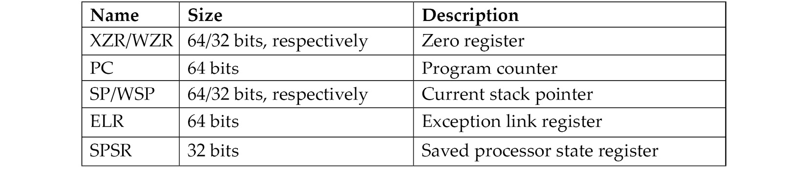
ARMv8 defines four exception levels (EL0-EL3), and each of the last three registers gets a copy of each; ELR and SPSR don’t have a separate copy of EL0.

There is no register called X31 or W31; the number 31 in many instructions represents either the zero register, ZR (WZR/XZR), or SP (for stack-related operations). X29 can be used as a frame pointer (which stores the original stack position), while X30 can be used as a link register (which stores a return value from the functions).

Regarding the calling convention, R0-R3 on the 32-bit ARM and X0-X7 on the 64-bit ARM are used to store argument values passed to functions with the remaining arguments passed through the stack – if necessary, R0-R1 and X0-X7 (and X8, also known as XR indirectly) to hold return results. If the type of the returned value is too big to fit them, then space needs to be allocated and returned as a pointer. Apart from this, R12 (32-bit) and X16- X17 (64-bit) can be used as intra-procedure-call scratch registers (by so-called veneers and procedure linkage table code) and R9 (32-bit) and X18 (64-bit) can be used as platform registers (for OS-specific purposes) if needed; otherwise, they are used the same way as other temporaries.

As mentioned previously, several CPU modes are implemented according to the official documentation, as follows:

Instruction sets

Several instruction sets are available for ARM processors: ARM and Thumb. A processor that is executing ARM instructions is said to be operating in the ARM state and vice versa. ARM processors always start in the ARM state; then, a program can switch to the Thumb state by using a BX instruction. Thumb Execution Environment (ThumbEE) was introduced relatively recently in ARMv7 and is based on Thumb, with some changes and additions to facilitate dynamically generated code.

ARM instructions are 32 bits long (for both AArch32 and AArch64), while Thumb and ThumbEE instructions are either 16 or 32 bits long (originally, almost all Thumb instructions were 16-bit, while Thumb-2 introduced a mix of 16 and 32-bit instructions).

All instructions can be split into the following categories according to the official documentation:

To interact with the OS, syscalls can be accessed using the Software Interrupt (SWI) instruction, which was later renamed the Supervisor Call (SVC) instruction.

See the official ARM documentation to get the exact syntax for any instruction. Here is an example of how it may look:

SVC{cond} #imm

In this case, the {cond} code will be a condition code. Several condition codes are supported by ARM, as follows:

• EQ: Equal to
• NE: Not equal to
• CS/HS: Carry set or unsigned higher or both
• CC/LO: Carry clear or unsigned lower
• MI: Negative
• PL: Positive or zero
• VS: Overflow
• VC: No overflow
• HI: Unsigned higher
• LS: Unsigned lower or both
• GE: Signed greater than or equal to
• LT: Signed less than
• GT: Signed greater than
• LE: Signed less than or equal to
• AL: Always (normally omitted)
• imm: It stands for the immediate value

Now, let's look at the basics of MIPS.

Basics of MIPS

Microprocessor without Interlocked Pipelined Stages (MIPS) was developed by MIPS Technologies (formerly MIPS computer systems). Similar to ARM, at first, it was a 32-bit architecture with 64-bit functionality added later. Taking advantage of the RISC ISA, MIPS processors are characterized by their low power and heat consumption. They can often be found in multiple embedded systems, such as routers and gateways. Several video game consoles such as Sony PlayStation also incorporated them. Unfortunately, due to the popularity of this architecture, the systems that implement it became a target of multiple IoT malware families. An example can be seen in the following screenshot:

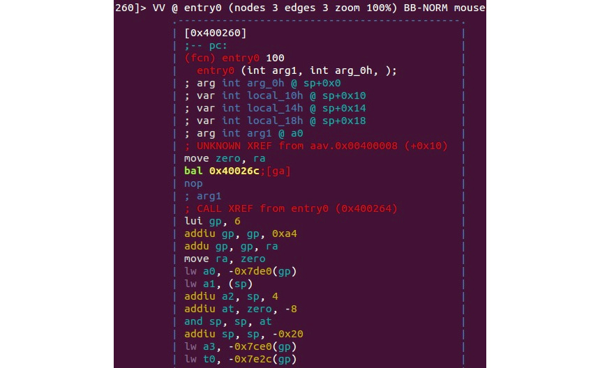
Figure 2.8 – IoT malware targeting MIPS-based systems

As the architecture evolved, there were several versions of it, starting from MIPS I and going up to V, and then several releases of the more recent MIPS32/MIPS64. MIPS64 remains backward compatible with MIPS32. These base architectures can be further supplemented with optional architectural extensions, called Application-Specific Extensions (ASEs), and modules to improve performance for certain tasks that are generally not used by the malicious code much. MicroMIPS32/64 are supersets of the MIPS32 and MIPS64 architectures, respectively, with almost the same 32-bit instruction set and additional 16-bit instructions to reduce the code size. They are used where code compression is required and are designed for microcontrollers and other small embedded devices.

Basics

MIPS supports bi-endianness. The following registers are available:

• 32 GPRs r0-r31 – 32-bit in size on MIPS32 and 64-bit in size on MIPS64.
• A special-purpose PC register that can be affected only indirectly by some instructions.
• Two special-purpose registers to hold the results of integer multiplication and division (HI and LO). These registers and their related instructions were removed from the base instruction set in the release of 6 and now exist in the Digital Signal Processor (DSP) module.

The reason behind 32 GPRs is simple – MIPS uses 5 bits to specify the register, so this way, we can have a maximum of 2^5 = 32 different values. Two of the GPRs have a particular purpose, as follows:

• Register r0 (sometimes referred to as $0 or $zero) is a constant register and always stores zero, and provides read-only access. It can be used as a /dev/null analog to discard the output of some operation, or as a fast source of a zero value.
• r31 (also known as $ra) stores the return address during the procedure call branch/jump and link instructions.

Other registers are generally used for particular purposes, as follows:

• r1 (also known as $at): Assembler temporary – used when resolving pseudo- instructions
• r2-r3 (also known as $v0 and $v1): Values – hold return function values.
• r4-r7 (also known as $a0-$a3): Arguments – used to deliver function arguments.
• r8-r15 (also known as $t0-$t7/$a4-$a7 and $t4-$t7): Temporaries – the first four can also be used to provide function arguments in N32 and N64 calling conventions (another O32 calling convention only uses r4-r7 registers; subsequent arguments are passed on the stack).
• r16-r23 (also known as $s0-$s7): Saved temporaries – preserved across function calls.
• r24-r25 (also known as $t8-$t9): Temporaries.
• r26-r27 (also known as $k0-$k1): Generally reserved for the OS kernel.
• r28 (also known as $gp): Global pointer – points to the global area (data segment).
• r29 (also known as $sp): Stack pointer.
• r30 (also known as $s8 or $fp): Saved value/frame pointer – stores the original stack pointer (before the function was called).

MIPS also has the following co-processors available:

• CP0: System control
• CP1: FPU
• CP2: Implementation-specific
• CP3: FPU (has dedicated COP1X opcode type instructions)

The instruction set

The majority of the main instructions were introduced in MIPS I and II. MIPS III introduced 64-bit integers and addresses, and MIPS IV and V improved floating-point operations and added a new set to boost the overall efficacy. Every instruction there has the same length – that is, 32 bits (4 bytes) – and all instructions start with an opcode that takes 6 bits. The three major instruction formats that are supported are R, I, and J:

For the FPU-related operations, the analogous FR and FI types exist.

Apart from this, several other less common formats exist, mainly coprocessors and extension-related formats.

In the documentation, registers usually have the following suffixes:

• Source (s)
• Target (t)
• Destination (d)

All instructions can be split into the following groups, depending on the functionality type:

• Control flow: This mainly consists of conditional and unconditional jumps and branches:
  • JR: Jump register (J format)
  • BLTZ: Branch on less than zero (I format)
• Memory access: Load and store operations:
  • LB: Load byte (I format)
  • SW: Store word (I format)
• ALU: Covers various arithmetic operations:
  • ADDU: Add unsigned (R format)
  • XOR: Exclusive or (R format)
  • SLL: Shift left logical (R format)
• OS interaction via exceptions: Interacts with the OS kernel:
  • SYSCALL: System call (custom format)
  • BREAK: Breakpoint (custom format)

Floating-point instructions will have similar names for the same types of operations in most cases, such as ADD.S. Some instructions are more unique, such as Check for Equal (C.EQ.D).

As we can see here and later, the same basic groups can be applied to virtually any architecture, and the only difference will be in their implementation. Some common operations may get instructions to benefit from optimizations and, in this way, reduce the size of the code and improve performance.

As the MIPS instruction set is pretty minimalistic, the assembler macros, known as pseudo instructions, also exist. Here are some of the most commonly used:

• ABS: Absolute value – translates into a combination of ADDU, BGEZ, and SUB
• BLT: Branch on less than – translates into a combination of SLT and BNE
• BGT/BGE/BLE: Similar to BLT
• LI/LA: Load immediate/address – translates into a combination of LUI and ORI or ADDIU for a 16-bit LI
• MOVE: Moves the content of one register into another – translates into ADD/ADDIU with a zero value
• NOP: No operation – translates into SLL with zero values
• NOT: Logical NOT – translates into NOR

Diving deep into PowerPC

PowerPC stands for Performance Optimization With Enhanced RISC—Performance Computing and is sometimes spelled as PPC. It was created in the early 1990s by the alliance of Apple, IBM, and Motorola (commonly abbreviated as AIM). It was originally intended to be used in PCs and powered Apple products, including PowerBooks and iMacs, up until 2006. The CPUs that implement it can also be found in game consoles such as Sony PlayStation 3, XBOX 360, and Wii, as well as in IBM servers and multiple embedded devices, such as car and plane controllers, and even in the famous ASIMO robot. Later, the administrative responsibilities were transferred to an open standards body, Power.org, where some of the former creators remained members, such as IBM and Freescale. The latter was separated from Motorola and later acquired by NXP Semiconductors. The OpenPOWER Foundation is a newer initiative by IBM, Google, NVIDIA, Mellanox, and Tyan that aims to facilitate collaboration in the development of this technology.

PowerPC was mainly based on IBM POWER ISA. Later, a unified Power ISA was released, which combined POWER and PowerPC into a single ISA that is now used in multiple products under the Power Architecture umbrella term.

There are plenty of IoT malware families that have payloads for this architecture.

Basics

The Power ISA is divided into several categories; each category can be found in a certain part of the specification or book. CPUs implement a set of these categories, depending on their class; only the base category is an obligatory one.

Here is a list of the main categories and their definitions in the latest second standard:

• Base: Covered in Book I (Power ISA User Instruction Set Architecture) and Book II (Power ISA Virtual Environment Architecture)
• Server: Covered in Book III-S (Power ISA Operating Environment Architecture –Server Environment)
• Embedded: Covered in Book III-E (Power ISA Operating Environment Architecture – Embedded Environment)

There are many more granular categories that cover aspects such as floating-point operations and caching for certain instructions.

Another book, Book VLE (Power ISA Operating Environment Architecture – Variable Length Encoding (VLE) Instructions Architecture), defines alternative instructions and definitions intended to increase the density of the code by using 16-bit instructions as opposed to the more common 32-bit ones.

Power ISA version 3 consists of three books with the same names as Books I to III of the previous standards, without distinctions between environments.

The processor starts in big-endian mode but can switch it by changing a bit in the Machine State Register (MSR) so that bi-endianness is supported.

Many sets of registers are documented in Power ISA, mainly grouped around either an associated facility or a category. Here is a basic summary of the most commonly used ones:

• 32 GPRs for integer operations, generally used by their number only (64-bit)
• 64 Vector Scalar Registers (VSRs) for vector operations and floating-point operations:
  • 32 Vector Registers (VRs) as part of the VSRs for vector operations (128-bit)
  • 32 FPRs as part of the VSRs for floating-point operations (64-bit)
• Special purpose fixed-point facility registers, such as the following:
  • Fixed-point exception register (XER), which contains multiple status bits (64-bit)
• Branch facility registers:
  • Condition Register (CR): Consists of eight 4-bit fields, CR0-CR7, involving things such as control flow and comparison (32-bit)
  • Link Register (LR): Provides the branch target address (64-bit)
  • Count Register (CTR): Holds a loop count (64-bit)
  • Target Access Register (TAR): Specifies the branch target address (64-bit)
• Timer facility registers:
  • Time Base (TB): This is incremented periodically with the defined frequency (64-bit)
• Other special-purpose registers from a particular category, including the following:
  • Accumulator (ACC) (64-bit): The Signal Processing Engine (SPE) category

Generally, functions can pass all arguments in registers for non-recursive calls; additional arguments are passed on the stack.

The instruction set

Most of the instructions are 32-bit; only the VLE group is smaller to provide a higher code density for embedded applications. All instructions are split into the following three categories:

• Defined: All of the instructions are defined in the Power ISA books.
• Illegal: Available for future extensions of the Power ISA. Attempting to execute them will invoke the illegal instruction error handler.
• Reserved: Allocated to specific purposes that are outside the scope of the Power ISA. Attempting to execute them will either result in an implemented action or invoke the illegal instruction error handler if the implementation is not available.

Bits 0 to 5 always specify the opcode, and many instructions also have an extended opcode. A large number of instruction formats are supported; here are some examples:

• I-FORM [OPCD+LI+AA+LK]
• B-FORM [OPCD+BO+BI+BD+AA+LK]

Each instruction field has an abbreviation and meaning; it makes sense to consult the official Power ISA document to get a full list of them and their corresponding formats. In terms of I-FORM, they are as follows:

• OPCD: Opcode
• LI: Immediate field used to specify a 24-bit signed two’s complement integer
• AA: Absolute address bit
• LK: Link bit affecting the link register

Instructions are also split into groups according to the associated facility and category, making them very similar to registers:

• Branch instructions:
  • b/ba/bl/bla: Branch
  • bc/bca/bcl/bcla: Branch conditional
  • sc: System call
• Fixed-point instructions:
  • lbz: Load byte and zero
  • stb: Store byte
  • addi: Add immediate
  • ori: OR immediate
• Floating-point instructions:
  • fmr: Floating move register
  • lfs: Load floating-point single
  • stfd: Store floating-point double
• SPE instructions:
  • brinc: Bit-reversed increment

Covering the SuperH assembly

SuperH, often abbreviated as SH, is a RISC ISA developed by Hitachi. SuperH went through several iterations, starting from SH-1 and moving up to SH-4. The more recent SH-5 has two modes of operation, one of which is identical to the user-mode instructions of SH-4, while another, SHmedia, is quite different. Each family has a market niche:

• SH-1: Home appliances
• SH-2: Car controllers and video game consoles such as Sega Saturn
• SH-3: Mobile applications such as car navigators
• SH-4: Car multimedia terminals and video game consoles such as Sega Dreamcast
• SH-5: High-end multimedia applications

Microcontrollers and CPUs that implement it are currently produced by Renesas Electronics, a joint venture of the Hitachi and Mitsubishi Semiconductor groups. As IoT malware mainly targets SH-4-based systems, we will focus on this SuperH family.

Basics

In terms of registers, SH-4 offers the following:

• 16 general registers R0-R15 (32-bit)
• Seven control registers (32-bit):
  • Global Base Register (GBR)
  • Status Register (SR)
  • Saved Status Register (SSR)
  • Saved Program Counter (SPC)
  • Vector Base Counter (VBR)
  • Saved General Register 15 (SGR)
  • Debug Base Register (DBR) (only from the privileged mode)
• Four system registers (32-bit):
  • MACH/MACL: Multiply-and-accumulate registers
  • PR: Procedure register
  • PC: Program counter
  • FPSCR: Floating-point status/control register
• 32 FPU registers – that is, FR0-FR15 (also known as DR0/2/4/... or FV0/4/...) and XF0-XF15 (also known as XD0/2/4/... or XMTRX); two banks of either 16 single-precision (32-bit) or eight double-precision (64-bit) FPRs and FPULs (floating-point communication registers) (32-bit)

Usually, R4-R7 are used to pass arguments to a function with the result returned in R0. R8-R13 are saved across multiple function calls. R14 serves as the frame pointer, while R15 serves as the stack pointer.

Regarding the data formats, in SH-4, a word takes 16 bits, a long word takes 32 bits, and a quadword takes 64 bits.

Two processor modes are supported: user mode and privileged mode. SH-4 generally operates in user mode and switches to privileged mode in case of an exception or an interrupt.

The instruction set

SH-4 features an instruction set that is upward-compatible with the SH-1, SH-2, and SH-3 families. It uses 16-bit fixed-length instructions to reduce the program code’s size. Except for BF and BT, all branch instructions and RTE (the return from exception instruction) implement so-called delayed branches, where the instruction following the branch is executed before the branch destination instruction.

All instructions are split into the following categories (with some examples):

• Fixed-point transfer instructions:
  • MOV: Move data (or particular data types specified)
  • SWAP: Swap register halves
• Arithmetic operation instructions:
  • SUB: Subtract binary numbers
  • CMP/EQ: Compare conditionally (in this case, on equal to)
• Logic operation instructions:
  • AND: Logical AND
  • XOR: Exclusive logical OR
• Shift/rotate instructions:
  • ROTL: Rotate left
  • SHLL: Shift logical left
• Branch instructions:
  • BF: Branch if false
  • JMP: Jump (unconditional branch)
• System control instructions:
  • LDC: Load to control register
  • STS: Store system register
• Floating-point single-precision instructions:
  • FMOV: Floating-point move
• Floating-point double-precision instructions:
  • FABS: Floating-point absolute value
• Floating-point control instructions:
  • LDS: Load to FPU system register
• Floating-point graphics acceleration instructions
  • FIPR: Floating-point inner product

Working with SPARC

Scalable Processor Architecture (SPARC) is a RISC ISA that was originally developed by Sun Microsystems (now part of the Oracle corporation). The first implementation was used in Sun’s own workstation and server systems. Later, it was licensed to multiple other manufacturers, one of them being Fujitsu. As Oracle terminated SPARC Design in 2017, all future development continued with Fujitsu as the main provider of SPARC servers.

Several fully open source implementations of the SPARC architecture exist. Multiple OSs currently support it, including Oracle Solaris, Linux, and BSD systems, and multiple IoT malware families have dedicated modules for it as well.

Basics

According to the Oracle SPARC architecture documentation, the implementation may contain between 72 and 640 general-purpose 64-bit R registers. However, only 31/32 GPRs are immediately visible at any one time; eight are global registers, R[0] to R[7] (also known as g0-g7), with the first register, g0, hardwired to 0; 24 are associated with the following register windows:

• Eight in registers in[0]-in[7] (R[24]-R[31]): For passing arguments and returning results
• Eight local registers local[0]-local[7] (R[16]-R[23]): For retaining local variables
• Eight out registers out[0]-out[7] (R[8]-R[15]): For passing arguments and returning results

The CALL instruction writes its address into the out[7] (R[15]) register.

To pass arguments to the function, they must be placed in the out registers. When the function gains control, it will access them in its registers. Additional arguments can be provided through the stack. The result is placed in the first register, which then becomes the first out register when the function returns. The SAVE and RESTORE instructions are used in this switch to allocate a new register window and restore the previous one, respectively.

SPARC also has 32 single-precision FPRs (32-bit), 32 double-precision FPRs (64-bit), and 16 quad-precision FPRs (128- bit), some of which overlap.

Apart from that, many other registers serve specific purposes, including the following:

• FPRS: Contains the FPU mode and status information
• Ancillary state registers (ASR 0, ASR 2-6, ASR 19-22, and ASR 24-28 are not reserved): These serve multiple purposes, including the following:
  • ASR 2: Condition Codes Register (CCR)
  • ASR 5: PC
  • ASR 6: FPRS
  • ASR 19: General Status Register (GSR)
• Register-Window PR state registers (PR 9-14): These determine the state of the register windows, including the following:
  • PR 9: Current Window Pointer (CWP)
  • PR 14: Window State (WSTATE)
• Non-register-Window PR state registers (PR 0-3, PR 5-8, and PR 16): Visible only to software running in privileged mode

32-bit SPARC uses big-endianness, while 64-bit SPARC uses big-endian instructions but can access data in any order. SPARC also uses the notion of traps, which implement a transfer of control to privileged software using a dedicated table that may contain the first eight instructions (32 for some frequently used traps) of each trap handler. The base address of the table is set by software in a Trap Base Address (TBA) register.

The instruction set

The instruction from the memory location, which is specified by the PC, is fetched and executed. Then, new values are assigned to the PC and the Next Program Counter (NPC), which is a pseudo-register.

Detailed instruction formats can be found in the individual instruction descriptions. Here are the basic categories of instructions supported, with examples:

• Memory access:
  • LDUB: Load unsigned byte
  • ST: Store
• Arithmetic/logical/shift integers:
  • ADD: Add
  • SLL: Shift left logical
• Control transfer:
  • BE: Branch on equal
  • JMPL: Jump and link
  • CALL: Call and link
  • RETURN: Return from the function
• State register access:
  • WRCCR: Write CCR
• Floating-point operations:
  • FOR: Logical OR for F registers
• Conditional move:
  • MOVcc: Move if the condition is true for the selected condition code (cc)
• Register window management:
  • SAVE: Save the caller’s window
  • FLUSHW: Flush register windows
• Single Instruction Multiple Data (SIMD) instructions:
  • FPSUB: Partitioned integer subtraction for F registers

Moving from assembly to high-level programming languages

Developers mostly don’t write in assembly. Instead, they write in higher-level languages, such as C or C++, and the compiler converts this high-level code into a low-level representation in assembly language. In this section, we will look at different code blocks represented in the assembly.

Arithmetic statements

Let’s look at different C statements and how they are represented in the assembly. We will use Intel IA-32 for this example. The same concept applies to other assembly languages as well:

• X = 50 (assuming 0x00010000 is the address of the X variable in memory):

  mov eax, 50

  mov dword ptr [00010000h], eax

• X = Y + 50 (assuming 0x00010000 represents X and 0x00020000 represents Y):

  mov eax, dword ptr [00020000h]

  add eax, 50

  mov dword ptr [00010000h], eax

• X = Y + (50 * 2):

  mov eax, dword ptr [00020000h]

  push eax    ; save Y for now

  mov eax, 50 ; do the multiplication first

  mov ebx, 2

  imul ebx    ; the result is in edx:eax

  mov ecx, eax

  pop eax     ; gets back Y value

  add eax, ecx

  mov dword ptr [00010000h], eax

• X = Y + (50 / 2):

  mov eax, dword ptr [00020000h]

  push eax ; save Y for now

  mov eax, 50

  mov ebx,2

  div ebx  ; the result is in eax, and the remainder is in edx

  mov ecx, eax

  pop eax

  add eax, ecx

  mov dword ptr [00010000h], eax

• X = Y + (50 % 2) (% represents the modulo):

  mov eax, dword ptr [00020000h]

  push eax ; save Y for now

  mov eax, 50

  mov ebx, 2

  div ebx  ; the remainder is in edx

  mov ecx, edx

  pop eax

  add eax, ecx

  mov dword ptr [00010000h], eax

Hopefully, this explains how the compiler converts these arithmetic statements into assembly language.

If conditions

Basic if statements may look like this:

• If (X == 50) (assuming 0x0001000 represents the X variable):

  mov eax, 50

  cmp dword ptr [00010000h], eax

• If (X & 00001000b) (| represents the logical AND):

  mov eax, 000001000b

  test dword ptr [00010000h], eax

To understand the branching and flow redirection, let’s look at the following diagram, which shows how it’s manifested in pseudocode:

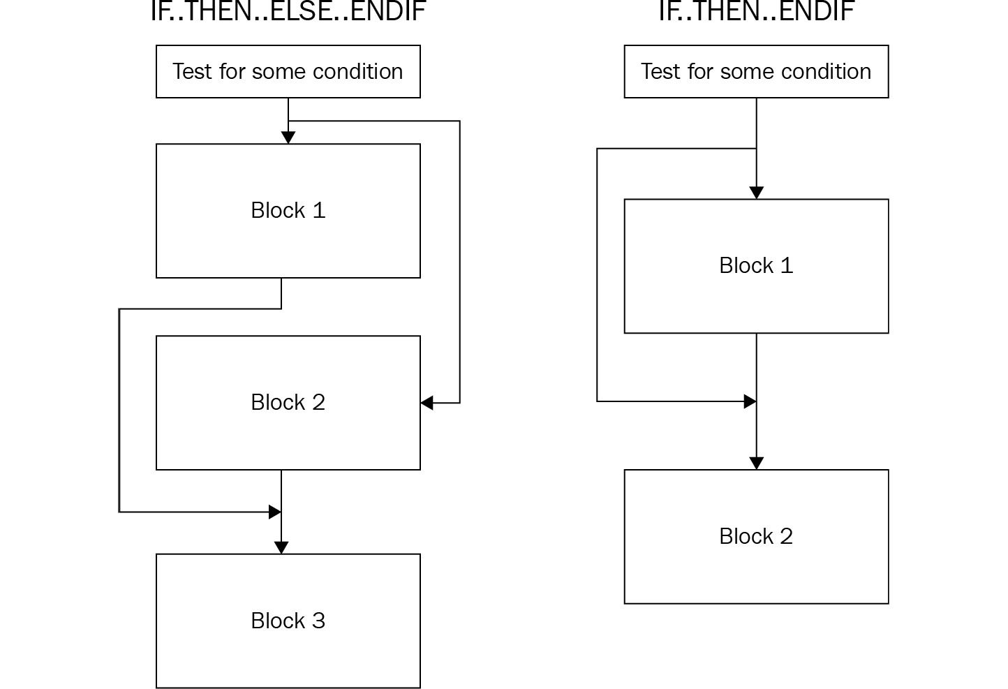
Figure 2.9 – Conditional flow redirection

To apply this branching sequence in assembly, the compiler uses a mix of conditional and unconditional jumps, as follows:

• IF.. THEN.. ENDIF:

  cmp dword ptr [00010000h], 50

  jnz 3rd_Block ; if not true

  …

  Some Code

  …

  3rd_Block:

  Some code

• IF.. THEN.. ELSE.. ENDIF:

  cmp dword ptr [00010000h], 50

  jnz Else_Block ; if not true

  ...

  Some code

  ...

  jmp 4th_Block  ; Jump after Else

  Else_Block:

  ...

  Some code

  ...

  4th_Block:

  ...

  Some code

While loop conditions

The while loop conditions are quite similar to if conditions in terms of how they are represented in assembly:

Summary

In this chapter, we covered the essentials of computer programming and described the universal elements that are shared between multiple CISC and RISC architectures. Then, we went through multiple assembly languages, including the ones behind Intel x86, ARM, MIPS, and others, and understood their application areas, which eventually shaped their design and structure. We also covered the fundamental basics of each of them, learned about the most important notions (such as the registers used and CPU modes supported), got an idea of how the instruction sets look, discovered what opcode formats are supported there, and explored what calling conventions are used. Finally, we went from the low-level assembly languages to their high-level representations in C or other similar languages and became familiar with a set of examples for universal blocks, such as if conditions and loops.

After reading this chapter, you should be able to read the disassembled code of different assembly languages and understand what high-level code it could represent. While not aiming to be completely comprehensive, the main goal of this chapter is to provide a strong foundation, as well as a direction that you can follow to deepen your knowledge before you analyze actual malicious code. It should be your starting point for learning how to perform static code analysis on different platforms and devices.

In Chapter 3, Basic Static and Dynamic Analysis for x86/x64, we will start analyzing the actual malware for particular platforms. The instruction sets we have become familiar with will be used as languages that describe their functionality.