3

Basic Static and Dynamic Analysis for x86/x64

In this chapter, we are going to cover the core fundamentals that you need to know to analyze 32-bit or 64-bit malware in the Windows platform. We will cover the Windows Portable Executable file header (PE header) and look at how it can help us to answer different incident handling and threat intelligence questions.

We will also walk through the concepts and basics of static and dynamic analysis, including processes and threads, the process creation flow, and WOW64 processes. Finally, we will cover process debugging, including setting breakpoints and altering the program’s execution.

This chapter will help you to perform basic static and dynamic analyses of malware samples by explaining the theory and equipping you with practical knowledge. By doing this, you will learn about the tools needed for malware analysis.

In this chapter, we will cover the following topics:

• Working with the PE header structure
• Static and dynamic linking
• Using PE header information for static analysis
• PE loading and process creation
• Basics of dynamic analysis using OllyDbg and x64dbg
• Debugging malicious services
• Essentials of behavioral analysis

Working with the PE header structure

When you start to perform basic static analysis on a file, your first valuable source of information will be the PE header. The PE header is a structure that any executable Windows file follows.

It contains various information, such as supported systems, the memory layouts of sections that contain code and data (such as strings, images, and so on), and various metadata, helping the system load and execute a file properly.

In this section, we will explore the PE header structure and learn how to analyze a PE file and read its information.

Why PE?

The portable executable structure was able to solve multiple issues that appeared in previous structures, such as MZ for MS-DOS executables. It represents a complete design for any executable file. Some of the features of the PE structure are as follows:

• It separates the code and the data into sections, making it easy to manage the data separately from the program and link any string back in the assembly code.
• Each section has separate memory permissions, which act as layers of security over the virtual memory of each program. These aim to allow or deny reading from a specific page of memory, writing to a specific page of memory, or executing code on a specific page of memory. A page of memory commonly takes 0x1000 bytes, which is 4,096 bytes in decimal.
• The file expands in memory (it takes less size on a hard disk), which allows you to create space for uninitialized variables (variables that don’t have a specific value assigned before the application uses them) and, at the same time, save space on the hard disk.
• It supports dynamic linking (via export and import directories), which is a very important technology that we will talk about later in this chapter.
• It supports relocation, which allows the program to be loaded in a different place in memory from what it was designed to be loaded in.
• It supports resource sections, where it can store any additional files, such as icons.
• It supports multiple processors, subsystems, and types of files, which allows the PE structure to be used across many platforms, such as Windows CE and Windows Mobile.

Now, let’s talk about what PE’s structure looks like.

Exploring PE’s structure

In this section, we will dive deeper into the structure of a typical executable file on a Windows operating system. This structure is used by Microsoft to represent multiple files, such as applications or libraries in the Windows operating system, across multiple types of devices, such as PCs, tablets, and mobile devices.

MZ header

Early in the MS-DOS era, Windows and DOS co-existed, and both had executable files with the same extension, .exe. So, each Windows application had to start with a small DOS application that printed a message stating This program cannot be run in DOS mode (or any similar message). This way, when a Windows application gets executed in the DOS environment, the small DOS application at the start of it will get executed and print this message to the user to run it in the Windows environment. The following diagram shows the high-level structure of the PE file header, with the DOS program’s MZ Header at the start:

Figure 3.1 – Example PE structure

This DOS header starts with the MZ magic value and ends with a field called e_lfanew, which points to the start of the portable executable header, or PE header.

PE header

The PE header starts with two letters, PE, followed by two important headers, which are the file header and the optional header. Later, all the additional structures are pointed to by the data directory array.

File header

Some of the most important values from this header are as follows:

Figure 3.2 – File header explained

The highlighted values are as follows:

1. Machine: This field represents the processor type – for example, 0x14c represents Intel 386 or later processors.
2. NumberOfSections: This value represents the number of sections that follow the headers, such as the code section, data section, or resources section (for files or images).
3. TimeDateStamp: This is the exact date and time that this program was compiled. It’s very useful for threat intelligence and creating a timeline of the attack.
4. Characteristics: This value represents the type of executable file and specifies whether it is a program or a dynamic link library (we will cover this later in this chapter).

Now, let’s talk about the optional header.

Optional header

Following the file header, the optional header comes with much more information, as shown here:

Figure 3.3 – Optional header explained

Here are some of the most important values in this header:

1. Magic: This identifies the platform the PE file supports (whether it’s x86 or x64).
2. AddressOfEntryPoint: This is a very important field for our analysis and it points to the starting point of program execution (to the first assembly instruction to be executed in the program) relative to its starting address (its base). These types of addresses are called Relative Virtual Addresses (RVAs).
3. ImageBase: This is the address where the program was designed to be loaded into virtual memory. All instructions that use absolute addresses will expect this as a program base. If the program has a relocation table, it can be loaded to a different base address. In this case, all such instructions will be updated by the Windows loader according to this table.
4. SectionAlignment: The size of each section and all header sizes should be aligned to this value when loaded into memory (generally, this value is 0x1000).
5. FileAlignment: The size of each section in the PE file (as well as the size of all headers) must be aligned to this number (for example, for a section that’s 0x1164 in size and has a file alignment value of 0x200, the section size will be changed to 0x1200 on the hard disk).
6. MajorSubsystemVersion: This represents the minimum Windows version to run the application on, such as Windows XP or Windows 7.
7. SizeOfImage: This is the size of the whole application in memory (usually, it’s larger than the size of the file on the hard disk due to uninitialized data, different alignments, and other reasons).
8. SizeOfHeaders: This is the size of all headers.
9. Subsystem: This indicates that this could be a Windows UI application, a console application, or a driver, or that it could even run on other Windows subsystems, such as Microsoft POSIX.

The optional header ends with a list of data directories.

Data directories

The data directory array points to a list of other structures that might be included in the executable and are not necessarily present in every application.

It includes 16 entries that follow the following format:

• Address: This points to the beginning of the structure in memory (from the start of the file).
• Size: This is the size of the corresponding structure.

The data directory includes many different values; not all of them are that important for malware analysis. Some of the most important entries to mention are as follows:

• Import directory: This represents the functions (or APIs) that this program doesn’t include but wants to import from other executable files or libraries (DLLs).
• Export directory: This represents the functions (or APIs) that this program includes in its code and is willing to export and allow other applications to use.
• Resource directory: This is always located at the start of the resource section and its purpose is to represent the packages’ files within the program, such as icons, images, and others.
• Relocation directory: This is always located at the start of the relocation section and it’s used to fix addresses in the code when the PE file is loaded to another place in memory.
• TLS directory: Thread Local Storage (TLS) points to functions that will be executed before the entry point. It can be used to bypass debuggers, as we will see later in greater detail.

Following the data directories, there is a section table.

Section table

After the 16 entries of the data directory array, there’s the section table. Each entry in the section table represents a section of the PE file. The number of sections in total is the number stored in the NumberOfSections field in FileHeader.

Here is an example of it:

Figure 3.4 – Example of a section table

These fields are used for the following purposes:

• Name: The name of the section (8 bytes max).
• VirtualSize: The size of a section (in memory).
• VirtualAddress: The pointer to the beginning of the section in memory (as RVA).
• SizeOfRawData: The size of a section (on the hard disk).
• PointerToRawData: The pointer to the beginning of the section in the file on the hard disk (relative to the start of the file). These types of addresses are called offsets.
• Characteristics: Memory protection flags (mainly EXECUTE, READ, or WRITE).

Now, let’s talk about the Rich header.

Rich header

This is a much lesser-known part of the MZ-PE header. It is located straight after the small DOS program, which prints the This program cannot be run in DOS mode string, and the PE header, as shown in the following screenshot:

Figure 3.5 – Raw Rich header

Unlike other header structures, it is supposed to be read from the end of where the Rich magic value is located. The value following it is the custom checksum that’s calculated over the DOS and Rich headers, which also serves as an XOR key, with which the actual content of this header is encrypted. Once decrypted, it will contain various information about the software that was used to compile the program. The very first field, once decrypted, will be the DanS marker:

Figure 3.6 – Parsed Rich header in the PE-Bear tool

This information can help researchers identify software that was used to create malware to choose the right tools for analysis and actor attribution.

As you can see, the PE structure is a treasure trove for malware analysts since it provides lots of invaluable information about both the malicious functionality and the attackers who created it.

PE+ (x64 PE)

At this point, you may be thinking that all x64 PE files’ fields take 8 bytes compared to 4 bytes in x86 PE files. But the truth is that the PE+ header is very similar to the good old PE header with very few changes, as follows:

• ImageBase: It is 8 bytes instead of 4 bytes.
• BaseOfData: This was removed from the optional header.
• Magic: This value changed from 0x10B (representing x86) to 0x20B (representing x64). PE+ files stayed at the maximum 2 GB size, while all other RVA addresses, including AddressOfEntrypoint, remained at 4 bytes.
• Some other fields, such as SizeOfHeapCommit, SizeOfHeapReserve, SizeOfStackReserve, and SizeOfStackCommit, now take 8 bytes instead of 4.

Now that we know what the PE header is, let’s talk about various tools that may help us extract and visualize this information.

PE header analysis tools

Once we become familiar with the PE format, we need to become able to parse different PE files (for example, .exe files) and read their header values. Luckily, we don’t have to do this ourselves in a hex editor; there are lots of different tools that can help us read PE header information easily. The most well-known free tools to do it are as follows:

• CFF Explorer: This tool is great for parsing the PE header as it properly analyzes and presents all the important information stored there:

Figure 3.7 – CFF Explorer UI

• PE-bear: The great advantage of this tool compared to CFF Explorer is that it can also parse the Rich header, which, as we know, contains lots of useful information about the developer tools used to create the sample.
• Hiew: While the demo version shows only a small subset of the PE header’s information, the full version gives researchers full visibility as well as the ability to edit any field there.
• PEiD: While it is mainly used to detect the compilers (Visual Studio, for example) or the packer that is used to pack this malware using static signatures stored within the application (this will be covered in greater detail in Chapter 4, Unpacking, Decryption, and Deobfuscation), researchers can use the > buttons to get lots of information from the PE header:

Figure 3.8 – PEiD UI

In the next section, we will further our knowledge and explore the nitty-gritty of static and dynamic linking.

Static and dynamic linking

In this section, we will cover the code libraries that were introduced to speed up the software development process, avoid code duplication, and improve the cooperation between different teams within companies producing software.

These libraries are a known target for malware families as they can easily be injected into the memory of different applications and impersonate them to disguise their malicious activities.

First of all, let’s talk about the different ways libraries can be used.

Static linking

With the increasing number of applications on different operating systems, developers found that there was a lot of code reuse and the same logic being rewritten over and over again to support certain functionalities in their programs. Because of that, the invention of code libraries came in handy. Let’s take a look at the following diagram:

Figure 3.9 – Static linking from compilation to loading

Code libraries (.lib files) include lots of functions to be copied to your program when required, so there is no need to reinvent the wheel and rewrite these functions again (for example, the code for mathematical operations such as sin or cos for any application that deals with mathematical equations). This is done by a program called a linker, whose job is to put all the required functions (groups of instructions) together and produce a single self-contained executable file as a result. This approach is called static linking.

Dynamic linking

Statically linked libraries lead to having the same code copied over and over again inside each program that may need it, which, in turn, leads to the loss of hard disk space and increases the size of the executable files.

In modern operating systems such as Windows and Linux, there are hundreds of libraries, and each contains thousands of functions for UIs, graphics, 3D, internet communications, and more. Because of that, static linking appeared to be limited. To mitigate this issue, dynamic linking emerged. The whole process is displayed in the following diagram:

Figure 3.10 – Dynamic linking from compilation to loading

Instead of storing the code inside each executable, any needed library is loaded next to each application in the same virtual memory so that this application can directly call the required functions. These libraries are named dynamic link libraries (DLLs), as shown in the preceding diagram. Let’s cover them in greater detail.

Dynamic link libraries

A DLL is a complete PE file that includes all the necessary headers, sections, and, most importantly, the export table.

The export table includes all the functions that this library exports. Not all library functions are exported as some of them are for internal use. However, the functions that are exported can be accessed through their names or ordinal numbers (index numbers). These are called application programming interfaces (APIs).

Windows provides lots of libraries for developers who are creating programs for Windows to access its functionality. Some of these libraries are as follows:

• kernel32.dll: This library includes the basic and core functionality for all programs, including reading a file and writing a file. In recent versions of Windows, the actual code of the functions moved to KernelBase.dll
• ntdll.dll: This library exports Windows native APIs; kernel32.dll uses this library as a backend for its functionality. Some malware writers try to access undocumented APIs inside this library to make it harder for reverse engineers to understand the malware functionality, such as LdrLoadDll.
• advapi32.dll: This library is used mainly for working with the registry and cryptography.
• shell32.dll: This library is responsible for shell-related operations such as executing and opening files.
• ws2_32.dll: This library is responsible for all the functionality related to internet sockets and network communications, which is very important for understanding custom network communication protocols.
• wininet.dll: This library contains HTTP and FTP functions and more.
• urlmon.dll: This library provides similar functionality to wininet.dll and is used for working with URLs, web compression, downloading files, and more.

Now, it’s time to talk about what exactly APIs are.

Application programming interface (API)

In short, APIs export functions in libraries that any application can call or interact with. In addition, APIs can be exported by executable files in the same way as DLLs. This way, an executable file can be run as a program or loaded as a library by other executables or libraries.

Each program’s import table contains the names of all the required libraries and all the APIs that this program uses. And in each library, the export table contains the API’s name, the API’s ordinal number, and the RVA address of this API.

Important Note

Each API has an ordinal number, but not all APIs have a name.

Dynamic API loading

In malware, it’s very common to obscure the name of the libraries and the APIs that they are using to hide their functionality from static analysis using what’s called dynamic API loading.

Dynamic API loading is supported by Windows using two very well-known APIs:

• LoadLibraryA: This API loads a dynamic link library into the virtual memory of the calling program and returns its address (variations include LoadLibraryW, LoadLibraryExA, and LoadLibraryExW).
• GetProcAddress: This API returns an address of the API specified by its name or the ordinal value and the address of the library that contains this API.

By calling these two APIs, malware can access APIs that are not written in the import table, which means they might be hidden from the eyes of the reverse engineer.

In some advanced malware, the malware author also hides the names of the libraries and the APIs using encryption or other obfuscation techniques, which will be covered in Chapter 4, Unpacking, Decryption, and Deobfuscation.

These APIs are not the only APIs that can allow dynamic API loading; other techniques will be explored in Chapter 8, Handling Exploits and Shellcode.

Armed with this knowledge, let’s learn more about how to put it into practice.

Using PE header information for static analysis

Now that we’ve covered the PE header, dynamic link libraries, and APIs, the question that arises is, How can we use this information in our static analysis? This depends on the questions that you want to answer, so that is what we will cover here.

How to use the PE header for incident handling

If an incident occurs, static analysis of the PE header can help you answer multiple questions in your report. Here are the questions and how the PE header can help you answer them:

• Is this malware packed?

The PE header can help you figure out if this malware is packed. Packers tend to change section names from their familiar names (.text, .data, and .rsrc) to something else, such as UPX0 or .aspack.

In addition, packers commonly hide most of the APIs otherwise expected to be present in the import table. So, if you see that the import table contains very few APIs, that could be another sign of packing being involved. We will cover unpacking in detail in Chapter 4, Unpacking, Decryption, and Deobfuscation.

• Is this malware a dropper or a downloader?

It’s very common to see droppers that have additional PE files stored in their resources. Multiple tools, such as Resource Hacker, can detect these embedded files (or, for example, a ZIP file that contains them), and you will be able to find the dropped modules.

For downloaders, it’s common to see an API named URLDownloadToFile from a DLL named urlmon.dll where you can download the file, and the ShellExecuteA API to execute the file. Other APIs can be used to achieve the same goal, but these two APIs are the most well-known and among the easiest to use for malware authors.

• Does it connect to the Command & Control server(s) (C&C, or the attacker’s website)? And how?

There are many APIs that can tell you that the malware uses the internet, such as socket, send, and recv, and they can tell you if they connect to a server acting as a client or if they listen to a port such as connect or listen, respectively.

Some APIs can even tell you what protocol they are using, such as HTTPSendRequestA or FTPPutFile, which are both from wininet.dll.

• What other functionalities does this malware have?

Some APIs are related to file searching, such as FindFirstFileA, which could be a hint that this malware may be ransomware or an info stealer.

It could use APIs such as Process32First, Process32Next, and CreateRemoteThread, which could mean a process injection functionality, or use TerminateProcess, which could mean that this malware may try to terminate other applications, such as antivirus programs or malware analysis tools.

We will cover all of these in greater detail later in this book. This section gave you hints and ideas to think about during your next static malware analysis and helped you find what you would be searching for in a PE header.

Usually, it is a good idea to focus on the main questions that you should answer in your report. Perhaps performing basic static analysis based on the strings and the PE header would be enough to help your case.

How to use a PE header for threat hunting

So far, we have covered how a PE header could help you answer questions related to incident handling or a normal tactical report. Now, let’s cover the following questions related to threat intelligence and how a PE header can help you answer them:

• When was this sample created?

Sometimes, threat researchers need to know how old the sample is. Is it an old sample or a new variant, and when did the attackers start to plan their attacks in the first place?

The PE header includes a value called TimeDateStamp in the file header. This value includes the exact date and time this sample was compiled, which can help answer this question and help threat researchers build their attack timeline. However, it’s worth mentioning that it can also be forged. Another less-known field that serves a similar purpose is the TimeDateStamp value of the Export Directory (when available).

• What’s the country of origin of these attackers?

What country do the attackers belong to? That can answer a lot about their motivations.

One of the ways to answer this question is, again, TimeDateStamp, which looks at many samples and their compile times. In some cases, they fall into 9-5 jobs for a particular time zone, which may help deduce the attackers’ country of origin, as shown in the following graph:

Figure 3.11 – Patterns in compilation timestamps

The Rich header may also be used for attribution purposes since combining different versions of software that were used to compile the sample generally doesn’t change very often for a particular setup.

• Is malware signed with a stolen certificate? Are all these samples related?

One of the data directory entries is related to the certificate. Some applications are signed by their manufacturer to provide additional trust for the users and the operating system that this application is safe. But these certificates sometimes get stolen and used by different malware actors.

For all the malicious samples that use a specific stolen certificate, it’s quite likely that all of them are produced by the same actor. Even if they have a different purpose or target different victims, they’re likely to be different activities performed by the same attackers.

As we mentioned earlier, a PE header is an information treasure trove if you look into the details hiding inside its fields. Here, we covered some of the most common use cases. There is so much more to get out of it, and it’s up to you to explore it further.

PE loading and process creation

Everything that we have covered so far was related to the PE file present on the hard disk. What we haven’t covered yet is how this PE file changes in memory when it’s loaded, as well as the whole execution process of these files. In this section, we will talk about how Windows loads a PE file, executes it, and turns it into a live program.

Basic terminology

To understand PE loading and process creation, we must cover some basic terminology, such as process, thread, Thread Environment Block (TEB), Process Environment Block (PEB), and others before we dive into the flow of loading and executing an executable PE file.

What’s a process?

A process is not just a representation of a running program in memory – it is also a container for all the information about the running application. This container stores information about the virtual memory associated with that process, all the loaded DLLs, opened files and sockets, the list of threads running as part of this process (we will cover this later), the process ID, and much more.

A process is a structure in the kernel that holds all this information, working as an entity to represent this running executable file, as shown in the following diagram:

Figure 3.12 – Example of a 32-bit process memory layout

We’ll compare the various aspects of virtual memory and physical memory in the next section.

Mapping virtual memory to physical memory

Virtual memory is like a holder for each process. Each process has its own virtual memory space to store its images, related libraries, and all the auxiliary memory ranges dedicated to the stack, heap, and so on. This virtual memory has a mapper to the equivalent physical memory. Not all virtual memory addresses are mapped to physical memory, and each one that’s been mapped has a permission (READ|WRITE, READ|EXECUTE, or maybe READ|WRITE|EXECUTE), as shown in the following diagram:

Figure 3.13 – Mappings between physical and virtual memory

Virtual memory allows you to create a security layer between one process and another and allows the operating system to manage different processes and suspend one process to give resources to another.

Threads

A thread is not just the entity that represents an execution path inside a process (and each process can have one or more threads running simultaneously). It is also a structure in the kernel that saves the whole state of that execution, including the registers, stack information, and the last error.

Each thread in Windows has a little time frame to run in before it gets stopped to have another thread resumed (as the number of processor cores is much smaller than the number of threads running in the entire system). When Windows changes the execution from one thread to another, it takes a snapshot of the whole execution state (registers, stack, instruction pointer, and so on) and saves it in the thread structure to be able to resume it again from where it stopped.

All threads running in one process share the same resources of that process, including the virtual memory, open files, open sockets, DLLs, mutexes, and others, and they synchronize with each other upon accessing these resources.

Each thread has a stack, instruction pointer, code functions for error handling (SEH, which will be covered in Chapter 6, Bypassing Anti-Reverse Engineering Techniques), a thread ID, and a thread information structure called TEB, as shown in the following diagram:

Figure 3.14 – Example processes with one and multiple threads

Next, we will talk about the crucial data structures that are needed to understand threads and processes. Let’s get started.

Important data structures – TIB, TEB, and PEB

The last thing that you need to understand related to processes and threads are TIB, TEB, and PEB data structures. These structures are stored inside the process memory, and their main function is to include all the information about the process and each thread, as well as make them accessible to the code so that it can easily know the process filename, the loaded DLLs, and other related information.

They can all be accessed through a special segment register, either FS (32-bit) or GS (64-bit), like this:

mov eax, DWORD PTR FS:[XX]

These data structures have the following functions:

• Thread Information Block (TIB): This contains information about the thread, including the list of functions that are used for error handling and much more.
• Thread Environment Block (TEB): This structure starts with the TIB, which is then followed by additional thread-related fields. In many cases, the terms TIB and TEB are used interchangeably.
• Process Environment Block (PEB): This includes various information about the process, such as its name, ID (PID), and a list of modules (which includes all the PE files that have been loaded in memory – mainly the program itself and the DLLs).

In the next section, and throughout this entire book, we will cover the different information that is stored in these structures that is used to help the malicious code achieve its goals – for example, to detect debuggers.

Process creation step by step

Now that we know the basic terminology, we can dive into PE loading and process creation. We will investigate it sequentially, as shown in the following steps:

1. Starting the program: When you double-click on a program in Windows Explorer, such as calc.exe, another process called explorer.exe (the process of Windows Explorer) calls an API, CreateProcessA, which gives the operating system the request to create this process and start its execution.
2. Creating the process data structures: Windows then creates the process data structure in the kernel (which is called EPROCESS), sets a unique ID for this process (ProcessID), and sets the explorer.exe file’s process ID as a parent PID for the newly created calc.exe process.
3. Initializing the virtual memory: After this, Windows creates the process, prepares the virtual memory, and saves its map inside the EPROCESS structure. Then, it creates the PEB structure with all the necessary information and loads the main two DLLs that Windows applications will always need: ntdll.dll and kernel32.dll (some applications run on other Windows subsystems, such as POSIX, and don’t use kernel32.dll).
4. Loading the PE file: After that, Windows starts loading the PE file (which we will explain next), which loads all the required third-party libraries (DLLs), including all the DLLs these libraries require, and makes sure to find the required APIs from these libraries and save their addresses in the import table of the loaded PE file so that the code can easily access them and call them.
5. Starting the execution: Last but not least, Windows creates the first thread in the process, which does some initialization and calls the PE file’s entry point to start the execution of the program. The TLS callbacks mentioned previously, if present, will be executed before the entry point.

Now, let’s dig deeper into the PE loading part of this process.

PE file loading step by step

The Windows PE loader follows these steps while loading an executable PE file into memory (including dynamic link libraries):

1. Parsing the headers: First, Windows starts by parsing the DOS header to find the PE header and then parses the PE header (file header and optional header) to gather some important information, such as the following:
   • ImageBase: To load the PE file (if possible) at this address in its virtual memory.
   • NumberOfSections: To be used to load the sections.
   • SizeOfImage: As this will be the final size of the whole PE file after being loaded in memory, this value will be used to allocate the space initially.
2. Parsing the section table: The NumberOfSections field parses all the sections in the PE file and makes sure to get all the necessary information, including their addresses and sizes in memory (VirtualAddress and VirtualSize respectively), as well as the offset and the size of the section on the hard disk for reading its data.
3. Mapping the file in memory: Using SectionAlignment, the loader copies all the headers and then moves each section to a new place using its VirtualAddress and VirtualSize values (if VirtualAddress or VirtualSize are not aligned with SectionAlignment, the loader will align them first and then use them), as shown in the following diagram:

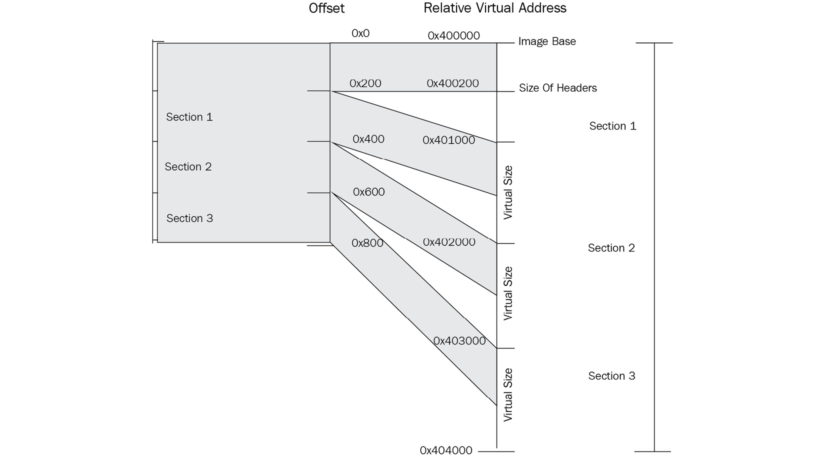
Figure 3.15 – Mapping sections from disk to memory

4. Dealing with third-party libraries: In this step, the loader loads all the required DLLs, going through this process again and again recursively until all DLLs are loaded. After that, it gets the addresses of all the imported APIs and saves them in the import table of the loaded PE file.
5. Dealing with relocation: If the program or any third-party library has a relocation table (in its data directory) and is loaded in a different place than its ImageBase, the loader fixes all the absolute addresses in the code with the new address of the program/library (with the new ImageBase).
6. Starting the execution: Finally, as in process creation, Windows creates the first thread, which executes the program from its entry point. Some anti-reverse engineering techniques can force it to start somewhere else before, which we will cover in Chapter 6, Bypassing Anti-Reverse Engineering Techniques.

One more thing we need to learn about is WOW64.

WOW64 processes

At this point, you should understand how a 32-bit process gets loaded into an x86 environment and how a 64-bit process gets loaded into an x64 environment. So, how about running 32-bit programs in 64-bit operating systems?

For this special case, Windows has created what’s called the WOW64 subsystem. It is implemented mainly in the following DLLs:

• wow64.dll
• wow64cpu.dll
• wow64win.dll

These DLLs create a simulated environment for the 32-bit process, which includes 32-bit versions of libraries that it may need.

These DLLs, rather than connecting directly to the Windows kernel, call an API, X86SwitchTo64BitMode, which then switches to x64 and calls the 64-bit ntdll.dll, which communicates directly with the kernel, as shown in the following diagram:

Figure 3.16 – WOW64 architecture

Also, for WOW64-based processes (x86 processes running in an x64 environment), new APIs were introduced, such as IsWow64Process, which is commonly used by malware to identify if it’s running as a 32-bit process in an x64 environment or an x86 environment.

Basics of dynamic analysis using OllyDbg and x64dbg

Now that we’ve explained processes, threads, and the execution of the PE files, it’s time to start debugging a running process and understanding its functionality by tracing over its code at runtime.

Debugging tools

There are multiple debugging tools we can use. Here, we will just give three examples that are quite similar to each other in terms of their UIs and functionality:

• OllyDbg: This is probably the most well-known debugger for the Windows platform. The following screenshot shows its UI, which has become a standard for most Windows debuggers:

Figure 3.17 – OllyDbg UI

• Immunity Debugger: This is a scriptable clone of OllyDbg that focuses on exploitation and bug hunting:

Figure 3.18 – Immunity Debugger UI

• X64dbg: This is a debugger for x86 and x64 executables with an interface that’s very similar to OllyDbg. It’s also an open source debugger:

Figure 3.19 – x64dbg UI

We will cover OllyDbg 1.10 (the most common version of OllyDbg) in great detail. The same concepts and hotkeys can be applied to other debuggers mentioned here.

How to analyze a sample with OllyDbg

The OllyDbg UI interface is pretty simple and easy to learn. In this section, we will cover the steps and the different windows that can help you with your analysis:

1. Select a sample to debug: You can directly open the sample file by going to File | Open and choosing a PE file to open (it could be a DLL file as well, but make sure it’s a 32-bit sample). Alternatively, you can attach it to a running process, as shown here:

Figure 3.20 – OllyDbg attaching dialog window

2. CPU window: This is your main window. This is the window that you spend most of your debugging time in. This window includes the assembly code in the top left-hand corner and provides the option to set breakpoints by double-clicking on the address or modifying the program’s assembly code.

You’ve also got the registers in the top right-hand corner. It is possible to modify them at any given time (once the execution has been paused). At the bottom, you have the stack and the data in hex format, which you can also modify.

You can simply modify any data in memory in the following two views:

Figure 3.21 – OllyDbg default window layout explained

3. Executable modules Window: There are multiple windows in OllyDbg that can help you with your analysis, such as the Executable modules window (you can access it by going to View | Executable modules), as shown in the following screenshot:

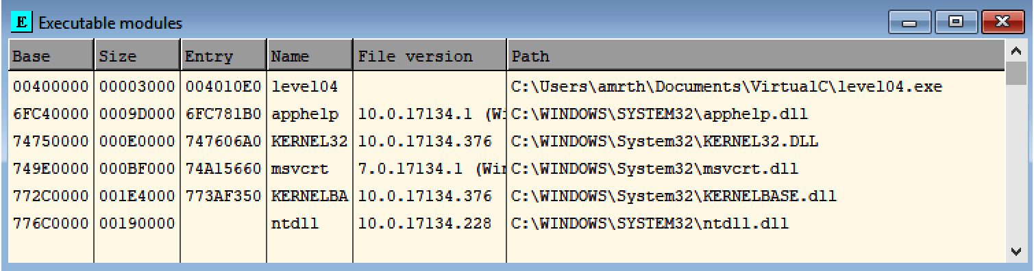
Figure 3.22 – OllyDbg dialog window for executable modules

This window will help you see all the loaded PE files in this process’ virtual memory, including the malware sample and all the libraries or DLLs loaded with it.

4. Memory map window: Here, you can see all the allocated memory inside the process’ virtual memory. Allocated memory is the memory that is represented in the physical (RAM) memory or a page file on the hard disk to store the content of the RAM when it’s not big enough. You can see what they represent and their memory protection (READ, WRITE, and/or EXECUTE), as shown in the following screenshot:

Figure 3.23 – OllyDbg memory map dialog window

5. Debugging the sample: In the Debug menu, you have multiple options for running the program’s assembly code, such as fully executing the sample until you hit a breakpoint using Run or just using F9.

The other option will be to just step over. Step over executes one line of code. However, if this line of code is a call to another function, it executes this function completely and stops just after the function returns. This makes it different from Step into, which goes inside the function and stops at the beginning of it, as shown in the following screenshot:

Figure 3.24 – OllyDbg debug menu

It includes the option to set hardware breakpoints and view them, which we will cover later in this chapter.

6. There’s much more: OllyDbg allows you to modify the code of the program; change its registers, state, and memory; dump any part of the memory; and save the changes of the PE file in memory back to the hard disk for further static analysis if needed.

Now, let’s talk about breakpoints.

Types of breakpoints

To be able to dynamically analyze a sample and understand its behavior, you need to be able to control its execution flow. You need to be able to stop the execution when a condition is met, examine its memory, and alter its registers’ values and instructions. There are several types of breakpoints that make this possible.

Step into/step over breakpoints

This breakpoint is very simple and allows the processor to execute only one instruction of the program, before returning to the debugger.

This breakpoint modifies a flag in a register called EFlags. While not common, this breakpoint could be detected by malware to identify the presence of a debugger, which we will cover when we look at anti-reverse engineering tricks in Chapter 6, Bypassing Anti-Reverse Engineering Techniques.

Software (INT3) breakpoints

This is the most common breakpoint, and you can easily set this breakpoint by double-clicking on the hex representation of an assembly line in the CPU window in OllyDbg or pressing F2. After this, you will see a red highlight over the address of this instruction, as shown in the following screenshot:

Figure 3.25 – Disassembly in OllyDbg

Well, this is what you see through the debugger’s UI, but what you don’t see is that the first byte of this instruction (0xB8, in this case) has been modified to 0xCC (the INT3 instruction), which stops the execution once the processor reaches it and returns control to the debugger. This 0xCC byte is not visible in the debugger UI as it keeps showing us the original bytes and the instruction they represent, but it can be seen if we decide to dump this memory on the disk and look at it using the hex editor.

Once the debugger gets control of this INT3 breakpoint, it replaces 0xCC with 0xB8 to execute this instruction normally.

The main problem with this breakpoint is that it modifies memory. If malware tries to read or modify the bytes of this instruction, it will read the first byte as 0xCC instead of 0xB8, which can break some code or detect the presence of the debugger (which we will cover in Chapter 6, Bypassing Anti-Reverse Engineering Techniques). In addition, it may affect memory dumping because this way, the resulting dump will be damaged by these modifications. The solution to this problem is to remove all software breakpoints before dumping memory.

Memory breakpoints

Memory breakpoints are used not to stop the execution of specific instructions, but to stop when any instruction tries to read or modify a specific part of memory. The way many debuggers set memory breakpoints is by adding the PAGE_GUARD (0x100) protection flag to the page’s original protection and removing PAGE_GUARD once the breakpoint is hit.

These can be accessed by right-clicking on Breakpoint | Memory, on access or Memory, on write, as shown in the following screenshot:

Figure 3.26 – OllyDbg breakpoint menu

Another important thing to note here is that memory breakpoints are less precise as it is only possible to change memory protection flags for a memory page, not for a single byte.

Hardware breakpoints

Hardware breakpoints are based on six special-purpose registers: DR0-DR3, DR6, and DR7.

These registers allow you to set a maximum of four breakpoints that have been given specific addresses to read, write, or execute 1, 2, or 4 bytes, starting from the given address. They are very useful as they don’t modify the instruction bytes as INT3 breakpoints do, and they are generally harder to detect. However, they could still be detected and removed by the malware, which we will discuss in Chapter 6, Bypassing Anti-Reverse Engineering Techniques.

You can view them from the Debug menu by going to Hardware breakpoints, as shown in the following screenshot:

Figure 3.27 – OllyDbg dialog window for hardware breakpoints

As you can see, each type of breakpoint serves a particular purpose and has advantages and disadvantages, so it is important to know all of them and use them according to the task at hand.

Modifying the program’s execution

To be able to bypass anti-debugging tricks, forcing the malware to communicate with the C&C or even testing different branches of the malware execution, you need to be able to alter the execution flow of the malware. Let’s look at the different techniques we can use to alter the execution flow and the behavior of any thread.

Modifying the program’s assembly instructions

You can modify the code execution path by changing the assembly instruction. For example, you can change a conditional jump instruction to the opposite condition, as shown in the following screenshot, and force the execution of a specific branch that wasn’t supposed to be executed:

Figure 3.28 – Working with assembly in OllyDbg

Apart from the code, it is also possible to change the content of registers.

Changing EFlags

Rather than modifying the code of the conditional jump instruction, you can modify the results of the comparison before it by changing the EFlags registers.

At the top right, after the registers, you have multiple flags that you can change. Each flag represents a specific result from any comparison (other instructions change these flags as well). For example, ZF represents if the two values are equal or if a register became zero. By changing the ZF flag, you force conditional jumps, such as jnz and jz, to jump to the opposite branch and force the execution path to change.

Modifying the instruction pointer value

You can force the execution of a specific branch or instruction by simply modifying the instruction pointer (EIP/RIP). You can do this by right-clicking on the instruction of interest and choosing New origin here.

Changing the program data

Just like you can change an instruction code, you can change the data values. With the bottom-left view (the hexadecimal view), you can change bytes of the data by right-clicking on Binary | Edit. You can also copy/paste hexadecimal values, as shown in the following screenshot:

Figure 3.29 – Data editing in OllyDbg

Now, let’s talk about how to efficiently search for important pieces of information to facilitate the analysis.

List strings, APIs, and cross-references

When performing reverse engineering, strings and APIs serve as very important sources of information, so it is important to know how to navigate them efficiently.

To get a list of strings in OllyDbg, right-click anywhere in the disassembly section of the CPU window and choose Search for | All referenced text strings. The resulting dialog box will show all candidate C-style strings, both ANSI and Unicode (UTF16-LE), and the instructions that use them.

To get a list of APIs, do the same, but this time, choose Search for | All intermodular calls.

Cross-references are markers that show the researcher where this code or data is being accessed. This is an extremely important piece of information that allows us to efficiently connect the dots. To find them for a particular instruction, right-click on it and choose the Find references to | Selected command option. For data in the hex dump window, it will be just Find references.

Setting labels and comments

When analyzing any kind of sample, it is important to keep the markup accurate so that you will always have a clear picture of what the meaning of already reviewed code or data is. Giving functions and references proper names is a great way to make sure you won’t have to re-analyze the same code again after some time.

To give the function or some data a name, right-click on its first instruction and choose the Label option (or just press the : hotkey). Now, all the references to them will use this label rather than an address, as shown in the following screenshot:

Figure 3.30 – Using labels and comments in OllyDbg

To follow the address, press Enter while selecting the instruction using it. To return, press the - hotkey. To leave comments, use the ; hotkey.

Now, let’s talk about x64dbg.

Differences between OllyDbg and x64dbg

As we mentioned previously, these debuggers share multiple similarities. They use the same layout and have pretty much the same interface options and hotkeys – even the default color schema is quite similar. However, there is a list of differences between them, some of which are worth mentioning:

• Unlike OllyDbg, x64dbg supports both 32- and 64-bit executables.
• By default, x64dbg stops at the system breakpoint (a system function that initializes an application to be debugged) while OllyDbg stops at the entry point.
• x64dbg supports tabs for dialog windows, which is very convenient in many cases, such as when several Hex dump windows must be used simultaneously.
• x64dbg displays more registers, including the DR0-3, DR6, and DR7 debug registers.
• OllyDbg may display incorrect protection flags in the Memory map window; x64dbg is generally more accurate.
• x64dbg displays breakpoints of all types in a single Breakpoints window while OllyDbg separates them into View | Breakpoints and Debug | Hardware breakpoints.
• x64dbg doesn’t have a menu option to call the DLL’s export function; it must be done manually.

There are other minor differences here and there, so feel free to try both tools and choose the one that suits you best.

Now, let’s talk about how to debug services.

Debugging malicious services

While loading individual executables and DLLs for debugging is generally a pretty straightforward task, things get a little bit more complicated when we talk about debugging Windows services.

What is a service?

Services are tasks that are generally supposed to execute certain logic in the background, similar to daemons on Linux. So, it comes as no surprise that malware authors commonly use them to achieve reliable persistence.

Services are controlled by the Service Control Manager (SCM), which is implemented in %SystemRoot%System32services.exe. All services have the corresponding HKLMSYSTEMCurrentControlSetservices<service_name> registry key. It contains multiple values that describe the service, including the following:

• ImagePath: A file path to the corresponding executable with optional arguments.
• Type: The REG_DWORD value specifies the type of the service. Let’s look at some examples of such supported values:
  • 0x00000001 (kernel): In this case, the logic is implemented in a driver (which will be covered in more detail in Chapter 7, Understanding Kernel-Mode Rootkits, which is dedicated to kernel-mode threats).
  • 0x00000010 (own): The service runs in its own process.
  • 0x00000020 (share): The service runs in a shared process.
• Start: This is another REG_DWORD value that describes the way the service is supposed to start. The following options are commonly used:
  • 0x00000000 (boot) and 0x00000001 (system): These values are used for drivers. In this case, they will be loaded by the boot loader or during the kernel’s initialization, respectively.
  • 0x00000002 (auto): The service will automatically start each time the machine restarts. This is the obvious choice for malware.
  • 0x00000003 (demand): This specifies a service that should be started manually. This option is particularly useful for debugging.
• 0x00000004 (disabled): The service won’t be started.

Let’s look at several ways the services can be designed:

• As an executable: Here, the actual logic is implemented in a dedicated executable file, and the previously mentioned ImagePath will contain its full file path.
• As a DLL (own loader): In this case, the service logic is located in a DLL that has its own loader (either a custom program or some standard one, such as rundll32.exe). The full command line is stored in the ImagePath key, the same as in the previous case.
• As a DLL (svchost): Here, instead of having its own EXE file, all service logic is implemented in a DLL that’s loaded into the address space of one of the svchost.exe processes. To be loaded, malware generally creates a new group in HKLMSOFTWAREMicrosoftWindows NTCurrentVersionSvchost registry key and passes this value to svchost.exe using the -k argument. The path to the DLL will be specified not in the ImagePath value of the service registry key, as in the previous case (here, it will contain the path of svchost.exe with the service group argument), but in the ServiceDll value of HKLMSYSTEMCurrentControlSetservices<service_name>Parameter s registry key. The service DLL should contain the ServiceMain export function (if the custom name is used, it should be specified in the ServiceMain registry value). If the SvchostPushServiceGlobals export is present, it will be executed before ServiceMain.

A user-mode service with a dedicated executable (or a DLL with its own loader) can be registered using the standard sc command-line tool, like this:

sc create <service_name> type= own binpath= <path_to_executable>

The process is slightly more complicated for svchost DLL-based services:

reg add "HKLMSOFTWAREMicrosoftWindows NTCurrentVersionSvchost" /v "<service_group>" /t REG_MULTI_SZ /d "<service_name>" /f
reg add "HKLMSYSTEMCurrentControlSetServices<service_name>Parameters"
/v ServiceDll /t REG_EXPAND_SZ /d <path_to_dll> /f sc create <service_name> type= share binpath= "C:WindowsSystem32svchost.exe -k <service_group>"

Using this approach, the created service can be started on demand, when necessary, such as by using the following command:

sc start <service_name>

Alternatively, you can use the following command:

net start <service_name_or_display_name>

Now, let’s talk about how we can attach to services.

Attaching to services

There are multiple ways to attach to services immediately once they start:

• Creating a dedicated registry key: It is possible to create a key such as HKLMSOFTWAREMicrosoftWindows NTCurrentVersionImage File Execution Options<filename> with the corresponding Debugger string data value, which contains the full path to the debugger to be attached to the service once the program with the specified <filename> starts. Here, there is the issue that the window of the attached debugger may not appear if the service is not interactive. It can be fixed in one of the following ways:
  • Open services.msc, open Properties for the debugged service, then go to the Log On tab and check the Allow service to interact with desktop option.
  • It can also be done manually by opening the type value of the HKLMSYSTEMCurrentControlSetservices<service_name> registry key and replacing its data with the result of a bitwise OR operation with the current value and the 0x00000100 DWORD (the SERVICE_INTERACTIVE_PROCESS flag). For example, 0x00000010 will become 0x00000110.
  • In addition, it can be created interactively when using the sc tool with the type= interact type= own or type= interact type= share arguments. Another option here is to use remote debugging.
• Using GFlags: The Global Flags Editor (GFlags) tool, which is part of the Debugging Tools for Windows (the same as WinDbg), provides multiple options for tweaking the process of debugging the candidate application. To attach the debugger, it modifies the registry key mentioned previously, so both approaches can be used pretty much interchangeably in this case. To do so using its UI, you must set the filename of the program of interest (not the full path) to the Image File tab and the Image field, and then refresh the window using the Tab key and set a tick against the Debugger field, where the full path to the debugger of preference should be specified. As in the previous case, you must make sure the service is interactive.
• Enabling child debugging: Here, it is possible to attach to services.exe with a debugger that supports breaks on the child process creation, enable it (for example, with the .childdbg 1 command in WinDbg), and then start the service of interest.
• Patching the entry point: The idea here is to put xEBxFE bytes on the entry point of the analyzed sample that represents the JMP instruction to redirect the execution to the start of itself, which creates an infinite loop. Then, it’s possible to find the corresponding process (it will consume a large number of CPU resources), attach to it with a debugger, restore the original bytes, and continue execution as usual while making sure that the restored instructions are successfully executed.

Once the debugger is attached, it is possible to place the breakpoint at the entry point of the sample to stop the execution there.

The common problem with debugging services is the timeout. By default, the service gets killed after about 30 seconds if it didn’t signal that it was executed successfully, which may complicate the debugging process. For example, WinDbg accidentally starts showing a No runnable debuggees error when trying to execute any command. To extend this time interval, you must create or update the DWORD ServicesPipeTimeout value in the HKLMSYSTEMCurrentControlSetControl registry key with the new timeout in milliseconds and restart the machine.

The service DLL’s exports, such as ServiceMain, can be debugged using any of the previously mentioned approaches. In this case, it is possible to either attach to the corresponding svchost.exe process immediately once it is created and enable breaking on the DLL load (for example, using the sxe ld[:<dll_name>] command in WinDbg) or patch the DLL’s entry point or any other export of interest with the infinite loop instruction and attach it to svchost.exe at any time once it’s started.

Finally, let’s explain what behavioral analysis is and how it can help us understand malware’s functionality.

Essentials of behavioral analysis

First of all, it is worth mentioning that some resources use the terms dynamic analysis and behavioral analysis interchangeably. Dynamic analysis is the process of executing instructions in the debugger, while behavioral analysis involves a black-box approach when malware is executed under various monitoring tools to record the changes it introduces. This approach allows researchers to get a quick insight into malware functionality. However, there are multiple limitations associated with it, as follows:

• Malware may execute only a part of its functionality
• Malware may behave differently if it notices it’s being analyzed

In most cases, behavioral analysis tools can easily be detected by various characteristics: file, process or directory names, registry keys and values, mutexes, window names, and so on.

Now, let’s look at the most commonly used tools, grouping them by type.

File operations

Here, the goal is to monitor all the changes that are introduced by malware at the filesystem level:

• Process Monitor (Filemon): Part of Sysinternals Suite, Process Monitor combines multiple previously standalone tools. One of them, formerly known as Filemon, allows you to record all filesystem operations that are performed by all processes:

Figure 3.31 – Various operations recorded by Process Monitor

• Sandboxie: The main purpose of this tool is to not just record file operations but to give the researchers access to created/modified files. This is extremely useful if malware drops or downloads additional modules and deletes them afterward.

Apart from file operations, monitoring registry operations is another proven by time technique that allows us to understand the purpose of malware.

Registry operations

In this case, we are interested in recording all the changes that have been made to the Windows Registry, a hierarchical database that stores various settings for both the operating systems and the applications that have been installed:

• Process Monitor (Regmon): This part of Process Monitor allows the researchers to record all types of actions that have been performed with the registry.
• Regshot: The idea of this tool is extremely simple – the researchers can create a snapshot of the registry before and after malware execution and compare them to see any differences that have been introduced:

Figure 3.32 – Regshot UI

• Autoruns: Another great tool from the Sysinternals Suite, it is invaluable for figuring out persistence mechanisms introduced by malware. It shows the researchers all the modules that will be loaded or executed once the system starts.

Now, let’s talk about process operations.

Process operations

Apart from monitoring registry and filesystem changes, any created or terminated processes are important artifacts from the malware analysis perspective. The following tools can help us keep track of them:

• Process Monitor (Procmon): Here, the researchers can keep an eye on all process-related operations – mainly their creation and termination.
• Process Explorer: This tool is also distributed as part of the Sysinternals Suite. In short, this is an advanced version of Task Manager that shows the process hierarchy (parent-child relationships) and more.

Another way to understand the purpose of malware is to track the APIs it uses.

WinAPIs

Here, instead of focusing on a particular type of activity, the researchers get the option to monitor specific Windows APIs by selecting any of them while grouped by functionality. To do that, the following tool can be used:

• API Monitor: This is a great tool that allows the researchers to select either individual APIs or their groups and see which of them were called by malware and in which order. Here is what its UI looks like:

Figure 3.33 – API Monitor groups WinAPIs by category

Finally, let’s talk about network operations.

Network activity

The following is a list of the most popular tools that allow us to get an insight into the network-related functionality of malware:

• Tcpview: This is quite a basic tool that shows the researchers all open ports, as well as established connections and their associated processes.
• Wireshark: The king of network traffic analysis, this tool gives invaluable insight into all sent and received packets and allows you to dissect them according to the OSI model and group them into streams. Its rich filtering syntax makes it an indispensable weapon for analyzing malicious network activity. The following screenshot shows what it looks like:

a

Figure 3.34 – Wireshark dissecting network packets

Instead of monitoring individual operations with separate tools manually, it is also possible to use sandboxes.

Sandboxes

Sandboxes are machines (usually virtual) that record all actions that have been performed by malware once it is executed, giving researchers a quick and detailed insight into its functionality. They may support various platforms, operating systems, and file types. Others may also record the generated traffic and collect memory dumps.

Like any behavioral analysis tool, there are multiple limitations associated with them, as follows:

• Sandboxes don’t know much about the environment that’s expected by malware and can’t automatically simulate, for example, the required command-line arguments.
• They can easily be detected. In this case, the malware may either immediately terminate or show some fake activity.
• Their visibility is limited as they commonly show only part of the malware functionality.

There are two options for using sandboxes:

• Online sandbox services

There are several big players in this market, some of which are commercial-only or public with subscription options. Here are some of the most well-known free public sandbox-based services:

• https://any.run
• https://www.hybrid-analysis.com
• https://virustotal.com (the Behavior tab)

Important Note

At the time of writing, VirusTotal supports multiple different sandboxes, so try a few different ones to find a good report.

• Self-managed sandboxes

Here, the researchers will need to host, set up, and administrate the software on their own, with all the corresponding pluses and minuses. Some of the most well-known options are as follows:

• Cuckoo (Free): Probably the most famous sandbox software, it has multiple forks, such as CAPE.
• DRAKVUF Sandbox (Free): The newer player in the sandbox market based on the DRAKVUF virtualization.
• VMRay (Commercial): Unlike the previous two, this one is commercial-only but provides outstanding results.

Depending on the use cases and the resources available, each option has its pros and cons and should be used accordingly.

This brings us to the end of this chapter. Now, let’s take a quick look at what we have learned and what we will cover in Chapter 4, Unpacking, Decryption, and Deobfuscation.

Summary

In this chapter, we covered the PE structure of Windows executable files. We covered the PE header field by field and examined its importance for static analysis, finishing with the main questions for incident handling and threat intelligence that the PE header of this sample can help us answer.

We also covered DLLs and how the PE files that reside together in the same virtual memory can communicate and share code and functions through what are called APIs. We also covered how import and export tables work.

Then, we covered dynamic analysis from its foundation, such as what a process is and what a thread is. We provided step-by-step guidance on how Windows creates a process and loads a PE file, from double-clicking on an application in Windows Explorer up until the program is running in front of you.

Last but not least, we covered how to dynamically analyze malware with OllyDbg by going through the most important functionalities of this tool to monitor, debug, and even modify the program’s execution. We talked about the different types of breakpoints, how to set them, how they work internally so that you can understand how they can be detected by malware, and how to bypass their anti-reverse engineering techniques. Finally, we covered Windows services and learned how they can be debugged.

At this point, you should have the foundation to perform basic malware analysis, including static and dynamic analysis. You should also have an understanding of what questions you need to answer in each step and the process you need to follow to have a full understanding of this malware’s functionality.

In Chapter 4, Unpacking, Decryption, and Deobfuscation, we will take our discussion and venture into unpacking, decryption, and deobfuscation into the context of malware. We will explore different techniques that have been introduced by malware authors to bypass detection and trick inexperienced reverse engineers. We will also learn how to bypass these techniques and deal with them.