
Chapter 6
Creating and Configuring Storage Devices
Storage has always been a critical element for any environment, and the storage infrastructure supporting vSphere is no different. This chapter will help you with all the elements required for a proper storage subsystem design, starting with vSphere storage fundamentals at the datastore and VM level and extending to best practices for configuring the storage array. Good storage design is critical for anyone building a virtual datacenter.
In this chapter, you will learn to
- Differentiate and understand the fundamentals of shared storage, including SANs and NAS
- Understand vSphere storage options
- Configure storage at the vSphere layer
- Configure storage at the VM layer
- Leverage best practices for SAN and NAS storage with vSphere
Reviewing the Importance of Storage Design
Storage design has always been important, but it becomes more so as vSphere is used for larger workloads, for mission-critical applications, for larger clusters, and as the basis for offerings based on Infrastructure as a Service (IaaS) in a nearly 100 percent virtualized datacenter. You can probably imagine why this is the case:
Advanced Capabilities Many of vSphere's advanced features depend on shared storage; vSphere High Availability (HA), vSphere Distributed Resource Scheduler (DRS), vSphere Fault Tolerance (FT), and VMware vCenter Site Recovery Manager all have a critical dependency on shared storage.
Performance People understand the benefits that virtualization brings—consolidation, higher utilization, more flexibility, and higher efficiency. But often, people have initial questions about how vSphere can deliver performance for individual applications when it is inherently consolidated and oversubscribed. Likewise, the overall performance of the VMs and the entire vSphere cluster both depend on shared storage, which is also highly consolidated and oversubscribed.
Availability The overall availability of your virtualized infrastructure—and by extension, the VMs running on that infrastructure—depend on the shared storage infrastructure. Designing high availability into this infrastructure element is paramount. If the storage is not available, vSphere HA will not be able to recover and the aggregate community of VMs can be affected. (We discuss vSphere HA in detail in Chapter 7, “Ensuring High Availability and Business Continuity.”)
While design choices at the server layer can make the vSphere environment relatively more or less optimal, design choices for shared resources such as networking and storage can sometimes make the difference between virtualization success and failure. This is especially true for storage because of its critical role. The importance of storage design and storage design choices remains true regardless of whether you are using storage area networks (SANs), which present shared storage as disks or logical units (LUNs); network attached storage (NAS), which presents shared storage as remotely accessed file systems; or a mix of both. Done correctly, you can create a shared storage design that lowers the cost and increases the efficiency, performance, availability, and flexibility of your vSphere environment.
This chapter breaks down these topics into the following main sections:
- “Examining Shared Storage Fundamentals” covers broad topics of shared storage that are critical with vSphere, including hardware architectures, protocol choices, and key terminology. Although these topics apply to any environment that uses shared storage, understanding these core technologies is a prerequisite to understanding how to apply storage technology in a vSphere implementation.
- “Implementing vSphere Storage Fundamentals” covers how storage technologies covered in the previous main section are applied and used in vSphere environments. This main section is broken down into a section on VMFS datastores (“Working with VMFS Datastores”), raw device mappings (“Working with Raw Device Mappings”), NFS datastores (“Working with NFS Datastores”), and VM-level storage configurations (“Working with VM-Level Storage Configuration”).
- “Leveraging SAN and NAS Best Practices” covers how to pull together all the topics discussed to move forward with a design that will support a broad set of vSphere environments.
Examining Shared Storage Fundamentals
vSphere 5.5 offers numerous storage choices and configuration options relative to previous versions of vSphere or to nonvirtualized environments. These choices and configuration options apply at two fundamental levels: the virtualization layer and the VM layer. The storage requirements for a vSphere environment and the VMs it supports are unique, making broad generalizations impossible. The requirements for any given vSphere environment span use cases ranging from virtual servers and desktops to templates and virtual CD/DVD (ISO) images. The virtual server use cases vary from light utility VMs with few storage performance considerations to the largest database workloads possible, with incredibly important storage layout considerations.
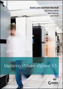
Let's start by examining this at a fundamental level. Figure 6.1 shows a simple three-host vSphere environment attached to shared storage.
It's immediately apparent that the ESXi hosts and the VMs will be contending for the shared storage asset. In a way similar to how ESXi can consolidate many VMs onto a single ESXi host, the shared storage consolidates the storage needs of all the VMs.
FIGURE 6.1 When ESXi hosts are connected to that same shared storage, they share its capabilities.
When sizing or designing the storage solution, you focus on attributes like capacity (gigabytes or terabytes) and performance, which is measured in bandwidth (megabytes per second, or MBps), throughput (I/O operations per second, or IOPS), and latency (in milliseconds). It goes sometimes without saying, but designing for availability, redundancy, and fault tolerance is also of paramount importance.
DETERMINING PERFORMANCE REQUIREMENTS
How do you determine the storage performance requirements of an application that will be virtualized, a single ESXi host, or even a complete vSphere environment? There are many rules of thumb for key applications, and the best practices for every application could fill a book. Here are some quick considerations:
- Online transaction processing (OLTP) databases need low latency (as low as you can get, but a few milliseconds is a good target). They are also sensitive to input/output operations per second (IOPS), because their I/O size is small (4 KB to 8 KB). TPC-C and TPC-E benchmarks generate this kind of I/O pattern.
- Decision support system/business intelligence databases and SQL Server instances that support Microsoft Office SharePoint Server need high bandwidth, which can be hundreds of megabytes per second because their I/O size is large (64 KB to 1 MB). They are not particularly sensitive to latency; TPC-H benchmarks generate the kind of I/O pattern used by these use cases.
- Copying files, deploying from templates, using Storage vMotion, and backing up VMs (within the guest or from a proxy server via vSphere Storage APIs) without using array–based approaches generally all need high bandwidth. In fact, the more, the better.
So, what does vSphere need? The answer is basic—the needs of the vSphere environment are the aggregate sum of all the use cases across all the VMs, which can cover a broad set of requirements. If the VMs are all small-block workloads and you don't do backups inside guests (which generate large-block workloads), then it's all about IOPS. If the VMs are all large-block workloads, then it's all about MBps. More often than not, a virtual datacenter has a mix, so the storage design should be flexible enough to deliver a broad range of capabilities and capacity—but without overbuilding.
How can you best determine what you will need? With small workloads, too much planning can result in overbuilding. You can use simple tools, including VMware Capacity Planner, Windows Perfmon, and top in Linux, to determine the I/O pattern of the applications and OSes that will be virtualized.
Also, if you have many VMs, consider the aggregate performance requirements, and don't just look at capacity requirements. After all, 1000 VMs with 10 IOPS each need an aggregate of 10000 IOPS, which is 50 to 80 fast spindle's worth, regardless of the capacity (in gigabytes or terabytes) needed.
Use large pool designs for generic, light workload VMs.
Conversely, focused, larger VM I/O workloads (such as virtualized SQL Server instances, SharePoint, Exchange, and other use cases) should be where you spend some time planning and thinking about layout. There are numerous VMware published best practices and a great deal of VMware partner reference architecture documentation that can help with virtualizing Exchange, SQL Server, Oracle, and SAP workloads. We have listed a few resources for you:
- Exchange
www.vmware.com/solutions/business-critical-apps/exchange/index.html
- SQL Server
www.vmware.com/solutions/business-critical-apps/sql-virtualization/overview.html
- Oracle
www.vmware.com/solutions/business-critical-apps/oracle-virtualization/index.html
- SAP
www.vmware.com/solutions/business-critical-apps/sap-virtualization/index.html
As with performance, the overall availability of the vSphere environment and the VMs depends on the same shared storage infrastructure, so a robust design is paramount. If the storage is not available, vSphere HA will not be able to recover and the consolidated community of VMs will be affected.
Note that we said the “consolidated community of VMs.” That statement underscores the need to put more care and focus on the availability of the configuration than on the performance or capacity requirements. In virtual configurations, the availability impact of storage issues is more pronounced, so you must use greater care in an availability design than in the physical world. It's not just one workload being affected—it's multiple workloads.
At the same time, advanced vSphere options such as Storage vMotion and advanced array techniques allow you to add, move, or change storage configurations nondisruptively, making it unlikely that you'll create a design where you can't nondisruptively fix performance issues.
Before going too much further, it's important to cover several basics of storage:
- Local storage versus shared storage
- Common storage array architectures
- RAID technologies
- Midrange and enterprise storage array design
- Protocol choices
We'll start with a brief discussion of local storage versus shared storage.
Comparing Local Storage with Shared Storage
An ESXi host can have one or more storage options actively configured, including the following:
- Local SAS/SATA/SCSI storage
- Fibre Channel
- Fibre Channel over Ethernet (FCoE)
- iSCSI using software and hardware initiators
- NAS (specifically, NFS)
- InfiniBand
Traditionally, local storage has been used in a limited fashion with vSphere because so many of vSphere's advanced features—such as vMotion, vSphere HA, vSphere DRS, and vSphere FT—required shared external storage. With vSphere Auto Deploy and the ability to deploy ESXi images directly to RAM at boot time coupled with host profiles to automate the configuration, in some environments local storage from vSphere 5.0 serves even less of a function than it did in previous versions.
With vSphere 5.0, VMware introduced a way to utilize local storage though the installation of a virtual appliance called the vSphere Storage Appliance, or simply VSA. At a high level, the VSA takes local storage and presents it back to ESXi hosts as a shared NFS mount. There are some limitations however. It can be configured with only two or three hosts, there are strict rules around the hardware that can run the VSA, and on top of this, it is licensed as a separate product. While it does utilize the underused local storage of servers, the use case for the VSA simply is not valid for many organizations.
vSphere 5.5, however, has two new features that are significantly more relevant to organizations than the VSA. vSphere Flash Read Cache and VSAN both take advantage of local storage, in particular, local flash storage. vSphere Flash Read Cache takes flash-based storage and allows administrators to allocate portions of it as a read cache for VM read I/O. VSAN extends on the idea behind the VSA and presents the local storage as a distributed datastore across many hosts. While this concept is similar to the VSA, the use of a virtual appliance is not required, nor are NFS mounts; it's entirely built into the ESXi hypervisor. Think of this as shared internal storage. Later in this chapter we'll explain how VSAN works and you can find information on vSphere Flash Read Cache in Chapter 11, “Managing Resource Allocation.”
So, how carefully do you need to design your local storage? The answer is simple—generally speaking, careful planning is not necessary for storage local to the ESXi installation. ESXi stores very little locally, and by using host profiles and distributed virtual switches, it can be easy and fast to replace a failed ESXi host. During this time, vSphere HA will make sure the VMs are running on the other ESXi hosts in the cluster. However, taking advantage of new features within vSphere 5.5 such as VSAN will certainly require careful consideration. Storage underpins your entire vSphere environment. Make the effort to ensure that your shared storage design is robust, taking into consideration internal- and external-based shared storage choices.
![]() Real World Scenario
Real World Scenario
NO LOCAL STORAGE? NO PROBLEM!
What if you don't have local storage? (Perhaps you have a diskless blade system, for example.) There are many options for diskless systems, including booting from Fibre Channel/iSCSI SAN and network-based boot methods like vSphere Auto Deploy (discussed in Chapter 2, “Planning and Installing VMware ESXi”). There is also the option of using USB boot, a technique that we've employed on numerous occasions in lab and production environments. Both Auto Deploy and USB boot give you some flexibility in quickly reprovisioning hardware or deploying updated versions of vSphere, but there are some quirks, so plan accordingly. Refer to Chapter 2 for more details on selecting the configuration of your ESXi hosts.
Shared storage is the basis for most vSphere environments because it supports the VMs themselves and because it is a requirement for many of vSphere's features. Shared external storage in SAN configurations (which encompasses Fibre Channel, FCoE, and iSCSI) and NAS (NFS) is always highly consolidated. This makes it efficient. SAN/NAS or VSAN can take the direct attached storage in physical servers that are 10 percent utilized and consolidate them to 80 percent utilization.
As you can see, shared storage is a key design point. Whether it's shared external storage or you're planning to share the local storage system out, it's important to understand some of the array architectures that vendors use to provide shared storage to vSphere environments. The high-level overview in the following section is neutral on specific storage array vendors because the internal architectures vary tremendously.
Defining Common Storage Array Architectures
This section is remedial for anyone with basic storage experience, but it's needed for vSphere administrators with no storage knowledge. For people unfamiliar with storage, the topic can be a bit disorienting at first. Servers across vendors tend to be relatively similar, but the same logic can't be applied to the storage layer because core architectural differences between storage vendor architectures are vast. In spite of that, storage arrays have several core architectural elements that are consistent across vendors, across implementations, and even across protocols.
The elements that make up a shared storage array consist of external connectivity, storage processors, array software, cache memory, disks, and bandwidth:
External Connectivity The external (physical) connectivity between the storage array and the hosts (in this case, the ESXi hosts) is generally Fibre Channel or Ethernet, though InfiniBand and other rare protocols exist. The characteristics of this connectivity define the maximum bandwidth (given no other constraints, and there usually are other constraints) of the communication between the ESXi host and the shared storage array.
Storage Processors Different vendors have different names for storage processors, which are considered the brains of the array. They handle the I/O and run the array software. In most modern arrays, the storage processors are not purpose-built application-specific integrated circuits (ASICs) but instead are general-purpose CPUs. Some arrays use PowerPC, some use specific ASICs, and some use custom ASICs for specific purposes. But in general, if you cracked open an array, you would most likely find an Intel or AMD CPU.
Array Software Although hardware specifications are important and can define the scaling limits of the array, just as important are the functional capabilities the array software provides. The capabilities of modern storage arrays are vast—similar in scope to vSphere itself—and vary wildly among vendors. At a high level, the following list includes some examples of these array capabilities and key functions:
- Remote storage replication for disaster recovery. These technologies come in many flavors with features that deliver varying capabilities. These include varying recovery point objectives (RPOs)—which reflect how current the remote replica is at any time, ranging from synchronous to asynchronous and continuous. Asynchronous RPOs can range from less than minutes to more than hours, and continuous is a constant remote journal that can recover to varying RPOs. Other examples of remote replication technologies are technologies that drive synchronicity across storage objects (or “consistency technology”), compression, and many other attributes, such as integration with VMware vCenter Site Recovery Manager.
- Snapshot and clone capabilities for instant point-in-time local copies for test and development and local recovery. These also share some of the ideas of the remote replication technologies like “consistency technology,” and some variations of point-in-time protection and replicas also have TiVo-like continuous journaling locally and remotely where you can recover/copy any point in time.
- Capacity-reduction techniques such as archiving and deduplication.
- Automated data movement between performance/cost storage tiers at varying levels of granularity.
- LUN/file system expansion and mobility, which means reconfiguring storage properties dynamically and nondisruptively to add capacity or performance as needed.
- Thin provisioning, which typically involves allocating storage on demand as applications and workloads require it.
- Storage quality of service (QoS), which means prioritizing I/O to deliver a given MBps, IOPS, or latency.
The array software defines the “persona” of the array, which in turn impacts core concepts and behavior. Arrays generally have a “file server” persona (sometimes with the ability to do some block storage by presenting a file as a LUN) or a “block” persona (generally with no ability to act as a file server). In some cases, arrays are combinations of file servers and block devices.
Cache Memory Every array differs as to how cache memory is implemented, but all have some degree of nonvolatile memory used for various caching functions—delivering lower latency and higher IOPS throughput by buffering I/O using write caches and storing commonly read data to deliver a faster response time using read caches. Nonvolatility (meaning ability to survive a power loss) is critical for write caches because the data is not yet committed to disk, but it's not critical for read caches. Cached performance is often used when describing shared storage array performance maximums (in IOPS, MBps, or latency) in specification sheets. These results generally do not reflect real-world scenarios. In most real-world scenarios, performance tends to be dominated by the disk performance (the type and number of disks) and is helped by write caches in most cases, but only marginally by read caches (with the exception of large relational database management systems, which depend heavily on read-ahead cache algorithms). One vSphere use case that is helped by read caches is a situation where many boot images are stored only once (through the use of vSphere or storage array technology), but this is also a small subset of the overall VM I/O pattern.
Disks Arrays differ as to which type of disks (often called spindles) they support and how many they can scale to support. Drives are described according to two different attributes. First, drives are often separated by the drive interface they use: Fibre Channel, serial-attached SCSI (SAS), and serial ATA (SATA). In addition, drives—with the exception of enterprise flash drives (EFDs)—are described by their rotational speed, noted in revolutions per minute (RPM). Fibre Channel drives typically come in 15K RPM and 10K RPM variants, SATA drives are usually found in 5400 RPM and 7200 RPM variants, and SAS drives are usually 15K RPM or 10K RPM variants. Second, EFDs, which are now mainstream, are solid state and have no moving parts; therefore rotational speed does not apply. The type and number of disks are very important. Coupled with how they are configured, this determines how a storage object (either a LUN for a block device or a file system for a NAS device) performs. Shared storage vendors generally use disks from the same disk vendors, so this is an area of commonality across shared storage vendors. The following list is a quick reference on what to expect under a random read/write workload from a given disk drive:
- 7,200 RPM SATA: 80 IOPS
- 10K RPM SATA/SAS/Fibre Channel: 120 IOPS
- 15K RPM SAS/Fibre Channel: 180 IOPS
- A commercial solid-state drive (SSD) based on Multi-Level Cell (MLC) technology: 1,000–2,000 IOPS
- An Enterprise Flash Drive (EFD) based on Single-Level Cell (SLC) technology and much deeper, very high-speed memory buffers: 6,000–30,000 IOPS
Bandwidth (Megabytes per Second) Performance tends to be more consistent across drive types when large-block, sequential workloads are used (such as single-purpose workloads like archiving or backup to disk), so in these cases, large SATA drives deliver strong performance at a low cost.
Explaining RAID
Redundant Array of Inexpensive (sometimes “Independent”) Disks (RAID) is a fundamental and critical method of storing the same data several times. RAID is used to increase data availability (by protecting against the failure of a drive) and to scale performance beyond that of a single drive. Every array implements various RAID schemes (even if it is largely invisible in file server persona arrays where RAID is done below the file system, which is the primary management element).
Think of it this way: Disks are mechanical, spinning, rust-colored surfaces. The read/write heads are flying microns above the surface while reading minute magnetic field variations and writing data by affecting surface areas also only microns in size.
THE “MAGIC” OF DISK DRIVE TECHNOLOGY
It really is a technological miracle that magnetic disks work at all. What a disk does all day long is analogous to a pilot flying a 747 at 600 miles per hour 6 inches off the ground and reading pages in a book while doing it!
In spite of the technological wonder of hard disks, they have unbelievable reliability statistics. But they do fail—and fail predictably, unlike other elements of a system. RAID schemes address this by leveraging multiple disks together and using copies of data to support I/O until the drive can be replaced and the RAID protection can be rebuilt. Each RAID configuration tends to have different performance characteristics and different capacity overhead impact.
We recommend that you view RAID choices as a significant factor in your design. Most arrays layer additional constructs on top of the basic RAID protection. (These constructs have many different names, but common ones are metas, virtual pools, aggregates, and volumes.)
Remember, all the RAID protection in the world won't protect you from an outage if the connectivity to your host is lost, if you don't monitor and replace failed drives and allocate drives as hot spares to automatically replace failed drives, or if the entire array is lost. It's for these reasons that it's important to design the storage network properly, to configure hot spares as advised by the storage vendor, and to monitor for and replace failed elements. Always consider a disaster-recovery plan and remote replication to protect from complete array failure.
Let's examine the RAID choices:
RAID 0 This RAID level offers no redundancy and no protection against drive failure (see Figure 6.2). In fact, it has a higher aggregate risk than a single disk because any single disk failing affects the whole RAID group. Data is spread across all the disks in the RAID group, which is often called a stripe. Although it delivers fast performance, this is the only RAID type that is usually not appropriate for any production vSphere use because of the availability profile.
FIGURE 6.2 In a RAID 0 configuration, the data is striped across all the disks in the RAID set, providing very good performance but very poor availability.
RAID 1, 1+0, 0+1 These mirrored RAID levels offer high degrees of protection but at the cost of 50 percent loss of usable capacity (see Figure 6.3). This is versus the raw aggregate capacity of the sum of the capacity of the drives. RAID 1 simply writes every I/O to two drives and can balance reads across both drives (because there are two copies). This can be coupled with RAID 0 to form RAID 1+0 (or RAID 10), which mirrors a stripe set, or to form RAID 0+1, which stripes data across pairs of mirrors. This has the benefit of being able to withstand multiple drives failing, but only if the drives fail on different elements of a stripe on different mirrors, thus making RAID 1+0 more fault tolerant than RAID 0+1. The other benefit of a mirrored RAID configuration is that, in the case of a failed drive, rebuild times can be very rapid, which shortens periods of exposure.
FIGURE 6.3 This RAID 10 2+2 configuration provides good performance and good availability, but at the cost of 50 percent of the usable capacity.
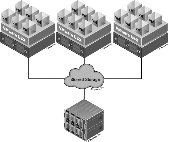
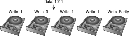
Parity RAID (RAID 5, RAID 6) These RAID levels use a mathematical calculation (an XOR parity calculation) to represent the data across several drives. This tends to be a good compromise between the availability of RAID 1 and the capacity efficiency of RAID 0. RAID 5 calculates the parity across the drives in the set and writes the parity to another drive. This parity block calculation with RAID 5 is rotated among the arrays in the RAID 5 set.
Parity RAID schemes can deliver very good performance, but there is always some degree of write penalty. For a full-stripe write, the only penalty is the parity calculation and the parity write, but in a partial-stripe write, the old block contents need to be read, a new parity calculation needs to be made, and all the blocks need to be updated. However, generally modern arrays have various methods to minimize this effect.
Read performance, on the other hand, is generally excellent because a larger number of drives can be read from than with mirrored RAID schemes. RAID 5 nomenclature refers to the number of drives in the RAID group, so Figure 6.4 would be referred to as a RAID 5 4+1 set. In the figure, the storage efficiency (in terms of usable to raw capacity) is 80 percent, which is much better than RAID 1 or 10.
FIGURE 6.4 A RAID 5 4+1 configuration offers a balance between performance and efficiency.
RAID 5 can be coupled with stripes, so RAID 50 is a pair of RAID 5 sets with data striped across them.
When a drive fails in a RAID 5 set, I/O can be fulfilled using the remaining drives and the parity drive, and when the failed drive is replaced, the data can be reconstructed using the remaining data and parity.
One downside to RAID 5 is that only one drive can fail in the RAID set. If another drive fails before the failed drive is replaced and rebuilt using the parity data, data loss occurs. The period of exposure to data loss because of the second drive failing should be mitigated.
The period of time that a RAID 5 set is rebuilding should be as short as possible to minimize the risk. The following designs aggravate this situation by creating longer rebuild periods:
- Very large RAID groups (think 8+1 and larger), which require more reads to reconstruct the failed drive.
- Very large drives (think 1 TB SATA and 500 GB Fibre Channel drives), which cause more data to be rebuilt.
- Slower drives that struggle heavily during the period when they are providing the data to rebuild the replaced drive and simultaneously support production I/O (think SATA drives, which tend to be slower during the random I/O that characterizes a RAID rebuild). The period of a RAID rebuild is actually one of the most stressful parts of a disk's life. Not only must it service the production I/O workload, but it must also provide data to support the rebuild, and it is known that drives are statistically more likely to fail during a rebuild than during normal duty cycles.
The following technologies all mitigate the risk of a dual drive failure (and most arrays do various degrees of each of these items):
- Using proactive hot sparing, which shortens the rebuild period substantially by automatically starting the hot spare before the drive fails. The failure of a disk is generally preceded with read errors (which are recoverable; they are detected and corrected using on-disk parity information) or write errors, both of which are noncatastrophic. When a threshold of these errors occurs before the disk itself fails, the failing drive is replaced by a hot spare by the array. This is much faster than the rebuild after the failure, because the bulk of the failing drive can be used for the copy and because only the portions of the drive that are failing need to use parity information from other disks.
- Using smaller RAID 5 sets (for faster rebuild) and striping the data across them using a higher-level construct.
- Using a second parity calculation and storing this on another disk.
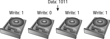
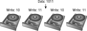
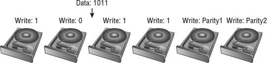
As described in the sidebar “A Key RAID 5 Consideration,” one way to protect against data loss in the event of a single drive failure in a RAID 5 set is to use another parity calculation. This type of RAID is called RAID 6 (RAID-DP is a RAID 6 variant that uses two dedicated parity drives, analogous to RAID 4). This is a good choice when large RAID groups and SATA are used.
Figure 6.5 shows an example of a RAID 6 4+2 configuration. The data is striped across four disks, and a parity calculation is stored on the fifth disk. A second parity calculation is stored on another disk. RAID 6 rotates the parity location with I/O, and RAID-DP uses a pair of dedicated parity disks. This provides good performance and good availability but a loss in capacity efficiency. The purpose of the second parity bit is to withstand a second drive failure during RAID rebuild periods. It is important to use RAID 6 in place of RAID 5 if you meet the conditions noted in the previous sidebar and are unable to otherwise use the mitigation methods noted.
FIGURE 6.5 A RAID 6 4+2 configuration offers protection against double drive failures.
While this is a reasonably detailed discussion of RAID levels, what you should take from it is that you shouldn't worry about it too much. Just don't use RAID 0 unless you have a proper use case for it. Use hot spare drives and follow the vendor best practices on hot spare density. EMC, for example, generally recommends one hot spare for every 30 drives in its arrays, whereas Compellent recommends one hot spare per drive type and per drive shelf. Just be sure to check with your storage vendor for their specific recommendations.
For most vSphere implementations, RAID 5 is a good balance of capacity efficiency, performance, and availability. Use RAID 6 if you have to use large SATA RAID groups or don't have proactive hot spares. RAID 10 schemes still make sense when you need significant write performance. Remember that for your vSphere environment it doesn't all have to be one RAID type; in fact, mixing different RAID types can be very useful to deliver different tiers of performance/availability.
For example, you can use most datastores with RAID 5 as the default LUN configuration, sparingly use RAID 10 schemes where needed, and use storage-based policy management, which we'll discuss later in this chapter, to ensure that the VMs are located on the storage that suits their requirements.
You should definitely make sure that you have enough spindles in the RAID group to meet the aggregate workload of the LUNs you create in that RAID group. The RAID type will affect the ability of the RAID group to support the workload, so keep RAID overhead (like the RAID 5 write penalty) in mind. Fortunately, some storage arrays can nondisruptively add spindles to a RAID group to add performance as needed, so if you find that you need more performance, you can correct it. Storage vMotion can also help you manually balance workloads.
Now let's take a closer look at some specific storage array design architectures that will impact your vSphere storage environment.
Understanding VSAN
vSphere 5.5 introduces a brand-new storage feature, virtual SAN, or simply VSAN. At a high level, VSAN pools the locally attached storage from members of a VSAN–enabled cluster and presents the aggregated pool back to all hosts within the cluster. This could be considered an “array” of sorts because just like a normal SAN, it has multiple disks presented to multiple hosts, but we would take it one step further and consider it an “internal array.” While VMware has announced VSAN as a new feature in vSphere 5.5, there are a few caveats. During the first few months of its availability it will be considered “beta only” and therefore not for production use. Also note that VSAN is licensed separately from vSphere itself.
As we mentioned earlier, in the section “Comparing Local Storage with Shared Storage,” VSAN does not require any additional software installations. It is built directly into ESXi. Managed from vCenter Server, VSAN is compatible with all the other cluster features that vSphere offers, such as vMotion, HA, and DRS. You can even use Storage DRS to migrate VMs on or off a VSAN datastore.
VSAN uses the disks directly attached to the ESXi hosts and is simple to set up, but there are a few specific requirements. Listed here is what you'll need to get VSAN up and running:
- ESXi 5.5 hosts
- vCenter 5.5
- One or more SSDs per host
- One or more HDDs per host
- Minimum of three hosts per VSAN cluster
- Maximum of eight hosts per VSAN cluster
- 1 Gbps network between hosts (10 Gbps recommended)
As you can see from the list, VSAN requires at least one flash-based device in each host. What may not be apparent from the requirements list is that the capacity of the SSD is not actually added to the overall usable space of the VSAN datastore. VSANs use the SSD as a read and write cache just as some external SANs do. When blocks are written to the underlying datastore, they are written to the SSDs first, and later the data can be relocated to the (spinning) HDDs if it's not considered to be frequently accessed.
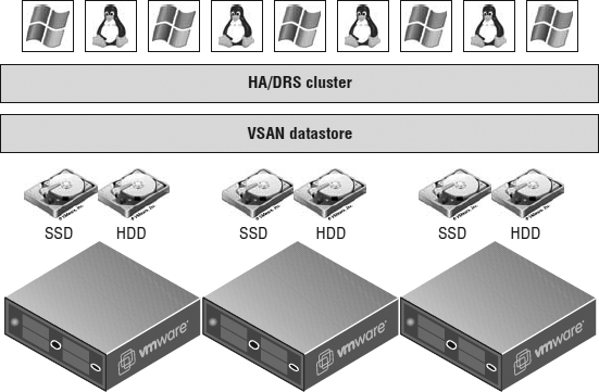
VSAN doesn't use the traditional RAID concepts that we explained in the previous section; it uses what VMware is calling RAIN, or Reliable Array of Independent Nodes. So, if there's no RAID, how do you achieve the expected reliability when using VSAN? VSAN uses a combination of VASA and Storage Service Policies to ensure that VMs are located on more than one disk and/or host to achieve their performance and availability requirements. This is why VMware recommends 10 Gbps networking between ESXi hosts when using VSAN. A VM's virtual disk could be located on one physical host but could be running on another host's CPU and memory. The storage system is fully abstracted from the compute resources, as you can see in Figure 6.6. In all likelihood the VMs virtual disk files could be located on multiple hosts in the cluster to ensure a level of redundancy.
FIGURE 6.6 VSAN abstracts the ESXi host's local disks and presents them to the entire VSAN cluster to consume.
Understanding Midrange and External Enterprise Storage Array Design
There are some major differences in physical array design that can be pertinent in a vSphere design.
Traditional external midrange storage arrays are generally arrays with dual-storage processor cache designs where the cache is localized to one storage processor or another but commonly mirrored between them. (Remember that all vendors call storage processors something slightly different; sometimes they are called controllers, heads, engines, or nodes.) In cases where one of the storage processors fails, the array remains available, but in general, performance is degraded (unless you drive the storage processors to only 50 percent storage processor utilization during normal operation).
External enterprise storage arrays are generally considered to be those that scale to many more controllers and a much larger global cache (memory can be accessed through some common shared model). In these cases, multiple elements can fail while the array is being used at a very high degree of utilization—without any significant performance degradation. Enterprise arrays can also include support for mainframes, and there are other characteristics that are beyond the scope of this book.
Hybrid designs exist as well, such as scale-out designs where they can scale out to more than two storage processors but without the features otherwise associated with enterprise storage arrays. Often these are iSCSI-only arrays and leverage iSCSI redirection techniques (which are not options of the Fibre Channel or NAS protocol stacks) as a core part of their scale-out design.
Design can be confusing, however, because VMware and storage vendors use the same words to express different things. To most storage vendors, an active-active storage array is an array that can service I/O on all storage processor units at once, and an active-passive design is a system where one storage processor is idle until it takes over for the failed unit. VMware has specific nomenclature for these terms that is focused on the model for a specific LUN. VMware defines active-active and active-passive arrays in the following way (this information is taken from the vSphere Storage Guide):
Active-Active Storage System An active-active storage system provides access to LUNs simultaneously through all available storage ports without significant performance degradation. Barring a path failure, all paths are active at all times.
Active-Passive Storage System In an active-passive storage system, one storage processor is actively providing access to a given LUN. Other processors act as backup for the LUN and can be actively servicing I/O to other LUNs. In the event of the failure of an active storage port, one of the passive storage processors can be activated to handle I/O.
Asymmetrical Storage System An asymmetrical storage system supports Asymmetric Logical Unit Access (ALUA), which allows storage systems to provide different levels of access per port. This permits the hosts to determine the states of target ports and establish priority for paths. (See the sidebar “The Fine Line between Active-Active and Active-Passive” for more details on ALUA.)
Virtual Port Storage System Access to all LUNs is provided through a single virtual port. These are active-active devices where the multiple connections are disguised behind the single virtual port. Virtual port storage systems handle failover and connection balancing transparently, which is often referred to as “transparent failover.”
This distinction between array types is important because VMware's definition is based on the multipathing mechanics, not whether you can use both storage processors at once. The active-active and active-passive definitions apply equally to Fibre Channel (and FCoE) and iSCSI arrays, and the virtual port definition applies to only iSCSI (because it uses an iSCSI redirection mechanism that is not possible on Fibre Channel/FCoE).
THE FINE LINE BETWEEN ACTIVE-ACTIVE AND ACTIVE-PASSIVE
Wondering why VMware specifies “without significant performance degradation” in the active-active definition? The reason is found within ALUA, a standard supported by many midrange arrays. vSphere supports ALUA with arrays that implement ALUA compliant with the SPC-3 standard.
Midrange arrays usually have an internal interconnect between the two storage processors used for write cache mirroring and other management purposes. ALUA was an addition to the SCSI standard that enables a LUN to be presented on its primary path and on an asymmetrical (significantly slower) path via the secondary storage processor, transferring the data over this internal interconnect.
The key is that the “non-optimized path” generally comes with a significant performance degradation. The midrange arrays don't have the internal interconnection bandwidth to deliver the same response on both storage processors because there is usually a relatively small, or higher-latency, internal interconnect used for cache mirroring that is used for ALUA versus enterprise arrays that have a very-high-bandwidth internal model.
Without ALUA, on an array with an active-passive LUN ownership model, paths to a LUN are shown as active, standby (designates that the port is reachable but is on a processor that does not have the LUN), and dead. When the failover mode is set to ALUA, a new state is possible: active non-optimized. This is not shown distinctly in the vSphere Web Client GUI, but it looks instead like a normal active path. The difference is that it is not used for any I/O.
So, should you configure your midrange array to use ALUA? Follow your storage vendor's best practice. For some arrays this is more important than others. Remember, however, that the non-optimized paths will not be used (by default) even if you select the Round Robin policy. An active-passive array using ALUA is not functionally equivalent to an active-passive array where all paths are used. This behavior can be different if using a third-party multipathing module—see the section “Reviewing Multipathing” later in this chapter.
By definition, all enterprise arrays are active-active arrays (by VMware's definition), but not all midrange arrays are active-passive. To make things even more confusing, not all active-active arrays (again, by VMware's definition) are enterprise arrays!
So, what do you do? What kind of array architecture is the right one for VMware? The answer is simple: All of them on VMware's Hardware Compatibility List (HCL) work; you just need to understand how the one you have works.
Most customers' needs are well met by midrange arrays, regardless of whether they have an active-active, active-passive, or virtual port (iSCSI-only) design or whether they are NAS devices. Generally, only the most mission-critical virtual workloads at the highest scale require the characteristics of enterprise-class storage arrays. In these cases, scale refers to VMs that number in the thousands, datastores that number in the hundreds, local and remote replicas that number in the hundreds, and the highest possible workloads—all that perform consistently even after component failures.
The most important considerations are as follows:
- If you have a midrange array, recognize that it is possible to oversubscribe the storage processors significantly. In such a situation, if a storage processor fails, performance will be degraded. For some customers, that is acceptable because storage processor failure is rare. For others, it is not, in which case you should limit the workload on either storage processor to less than 50 percent or consider an enterprise array.
- Understand the failover behavior of your array. Active-active arrays use the fixed-path selection policy by default, and active-passive arrays use the most recently used (MRU) policy by default. (See the section “Reviewing Multipathing” for more information.)
- Do you need specific advanced features? For example, if you want disaster recovery, make sure your array has integrated support on the VMware vCenter Site Recovery Manager HCL. Or, do you need array-integrated VMware snapshots? Do they have integrated management tools? More generally, do they support the vSphere Storage APIs? Ask your array vendor to illustrate its VMware integration and the use cases it supports.
We're now left with the last major area of storage fundamentals before we move on to discussing storage in a vSphere-specific context. The last remaining area deals with choosing a storage protocol.
Choosing a Storage Protocol
vSphere offers several shared storage protocol choices, including Fibre Channel, FCoE, iSCSI, and Network File System (NFS), which is a form of NAS. A little understanding of each goes a long way in designing the storage for your vSphere environment.
REVIEWING FIBRE CHANNEL
SANs are most commonly associated with Fibre Channel storage because Fibre Channel was the first protocol type used with SANs. However, SAN refers to a network topology, not a connection protocol. Although people often use the acronym SAN to refer to a Fibre Channel SAN, you can create a SAN topology using different types of protocols, including iSCSI, FCoE, and InfiniBand.
SANs were initially deployed to mimic the characteristics of local or direct attached SCSI devices. A SAN is a network where storage devices (logical units—or LUNs—just as on a SCSI or SAS controller) are presented from a storage target (one or more ports on an array) to one or more initiators. An initiator is usually a host bus adapter (HBA) or converged network adapter (CNA), though software-based initiators are available for iSCSI and FCoE. See Figure 6.7.
Today, Fibre Channel HBAs have roughly the same cost as high-end multiported Ethernet interfaces or local SAS controllers, and the per-port cost of a Fibre Channel switch is about twice that of a high-end managed Ethernet switch.
Fibre Channel uses an optical interconnect (though there are copper variants), which is used since the Fibre Channel protocol assumes a very high-bandwidth, low-latency, and lossless physical layer. Standard Fibre Channel HBAs today support very-high-throughput, 4 Gbps, 8 Gbps, and even 16 Gbps connectivity in single-, dual-, or quad-ported options. Older, obsolete HBAs supported up to only 2 Gbps. Some HBAs supported by ESXi are the QLogic QLE2462 and Emulex LP10000. You can find the authoritative list of supported HBAs on the VMware HCL at www.vmware.com/resources/compatibility/search.php. For end-to-end compatibility (in other words, from host to HBA to switch to array), every storage vendor maintains a similar compatibility matrix.
FIGURE 6.7 A Fibre Channel SAN presents LUNs from a target array (in this case an EMC VNX) to a series of initiators (in this case a Cisco Virtual Interface Controller).
Although in the early days of Fibre Channel there were many types of cables and interoperability of various Fibre Channel initiators, firmware revisions, switches, and targets (arrays) were not guaranteed, today interoperability is broad. Still, it is always a best practice to maintain your environment with the vendor interoperability matrix. From a connectivity standpoint, almost all cases use a common OM2 (orange-colored cables) multimode duplex LC/LC cable. The newer OM3 and OM4 (aqua-colored cables) are used for longer distances and are generally used for 10 Gbps Ethernet and 8/16 Gbps Fibre Channel (which otherwise have shorter distances using OM2). They all plug into standard optical interfaces.
The Fibre Channel protocol can operate in three modes: point-to-point (FC-P2P), arbitrated loop (FC-AL), and switched (FC-SW). Point-to-point and arbitrated loop are rarely used today. FC-AL is commonly used by some array architectures to connect their backend spindle enclosures (vendors give different hardware names to them, but they're the hardware elements that contain and support the physical disks) to the storage processors, but even in these cases, most modern array designs are moving to switched designs, which have higher bandwidth per disk enclosure.
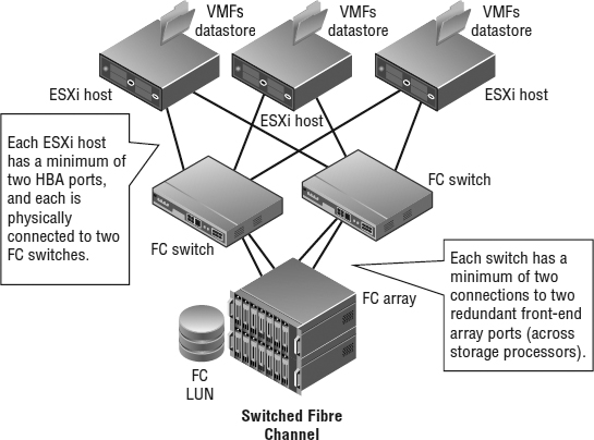
As Figure 6.8 shows, each ESXi host has a minimum of two HBA ports, and each is physically connected to two Fibre Channel switches. Each switch has a minimum of two connections to two redundant front-end array ports (across storage processors).
FIGURE 6.8 The most common Fibre Channel configuration: a switched Fibre Channel (FC-SW) SAN. This enables the Fibre Channel LUN to be easily presented to all the hosts while creating a redundant network design.
HOW DIFFERENT IS FCOE?
Aside from discussions of the physical media and topologies, the concepts for FCoE are almost identical to those of Fibre Channel. This is because FCoE was designed to be seamlessly interoperable with existing Fibre Channel–based SANs.
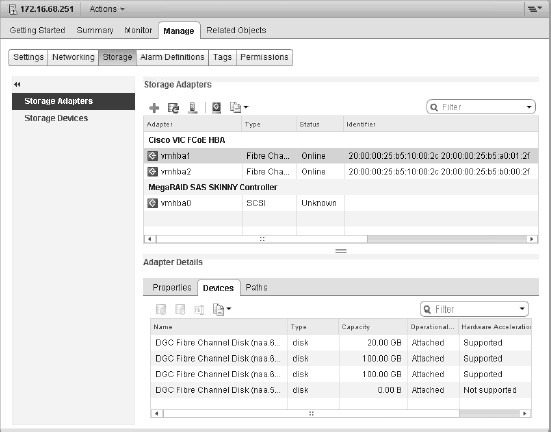
All the objects (initiators, targets, and LUNs) on a Fibre Channel SAN are identified by a unique 64-bit identifier called a worldwide name (WWN). WWNs can be worldwide port names (a port on a switch) or node names (a port on an endpoint). For anyone unfamiliar with Fibre Channel, this concept is simple. It's the same technique as Media Access Control (MAC) addresses on Ethernet. Figure 6.8 shows an ESXi host with FCoE CNAs, where the highlighted CNA has the following worldwide node name: worldwide port name (WWnN: WWpN) in the identifier column:
20:00:00:25:b5:10:00:2c 20:00:00:25:b5:a0:01:2f
Like Ethernet MAC addresses, WWNs have a structure. The most significant two bytes are used by the vendor (the four hexadecimal characters starting on the left) and are unique to the vendor, so there is a pattern for QLogic or Emulex HBAs or array vendors. In the previous example, these are Cisco CNAs connected to an EMC VNX storage array.
Fibre Channel and FCoE SANs also have a critical concept of zoning. Fibre Channel switches implement zoning to restrict which initiators and targets can see each other as if they were on a common bus. If you have Ethernet networking experience, the idea is somewhat analogous to non-routable VLANs with Ethernet.
IS THERE A FIBRE CHANNEL EQUIVALENT TO VLANS?
Actually, yes, there is. Virtual storage area networks (VSANs) were adopted as a standard in 2004. Like VLANs, VSANs provide isolation between multiple logical SANs that exist on a common physical platform. This enables SAN administrators greater flexibility and another layer of separation in addition to zoning. These are not to be confused with VMware's new VSAN feature described earlier in this chapter.
Zoning is used for the following two purposes:
- To ensure that a LUN that is required to be visible to multiple hosts in a cluster (for example in a vSphere cluster, a Microsoft cluster, or an Oracle RAC cluster) has common visibility to the underlying LUN while ensuring that hosts that should not have visibility to that LUN do not. For example, it's used to ensure that VMFS volumes aren't visible to Windows servers (with the exception of backup proxy servers using software that leverages the vSphere Storage APIs for Data Protection).
- To create fault and error domains on the SAN fabric, where noise, chatter, and errors are not transmitted to all the initiators/targets attached to the switch. Again, it's somewhat analogous to one of the uses of VLANs to partition very dense Ethernet switches into broadcast domains.
Zoning is configured on the Fibre Channel switches via simple GUIs or CLI tools and can be configured by port or by WWN:
- Using port-based zoning, you would zone by configuring your Fibre Channel switch to “put port 5 and port 10 into a zone that we'll call zone_5_10.” Any device (and therefore any WWN) you physically plug into port 5 could communicate only to a device (or WWN) physically plugged into port 10.
- Using WWN-based zoning, you would zone by configuring your Fibre Channel switch to “put WWN from this HBA and these array port WWNs into a zone we'll call ESXi_55_ host1_CX_SPA_0.” In this case, if you moved the cables, the zones would move to the ports with the matching WWNs.
The ESXi configuration shown in Figure 6.9 shows the LUN by its runtime or “shorthand” name. Masked behind this name is an unbelievably long name that that combines the initiator WWN, the Fibre Channel switch ports, and the Network Address Authority (NAA) identifier. This provides an explicit name that uniquely identifies not only the storage device but also the full end-to-end path.
We'll give you more details on storage object naming later in this chapter, in the sidebar titled “What Is All the Stuff in the Storage Device Details List?”
Zoning should not be confused with LUN masking. Masking is the ability of a host or an array to intentionally ignore WWNs that it can actively see (in other words, that are zoned to it). Masking is used to further limit what LUNs are presented to a host (commonly used with test and development replicas of LUNs).
You can put many initiators and targets into a zone and group zones together, as illustrated in Figure 6.10. For features like vSphere HA and vSphere DRS, ESXi hosts must have shared storage to which all applicable hosts have access. Generally, this means that every ESXi host in a vSphere environment must be zoned such that it can see each LUN. Also, every initiator (HBA or CNA) needs to be zoned to all the front-end array ports that could present the LUN. So, what's the best configuration practice? The answer is single initiator/single target zoning. This creates smaller zones, creates less cross talk, and makes it more difficult to administratively make an error that removes a LUN from all paths to a host or many hosts at once with a switch configuration error.
FIGURE 6.9 The Edit Multipathing Policies dialog box shows the storage runtime (short-hand) name.
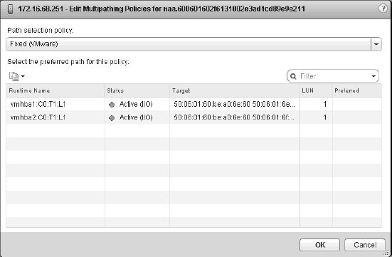
FIGURE 6.10 There are many ways to configure zoning. From left to right: multi-initiator/multi-target zoning, single-initiator/multi-target zoning, and single-initiator/single-target zoning.
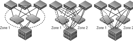
Remember that the goal is to ensure that every LUN is visible to all the nodes in the vSphere cluster. The left side of the figure is how most people who are not familiar with Fibre Channel start—multi-initiator zoning, with all array ports and all the ESXi Fibre Channel initiators in one massive zone. The middle is better—with two zones, one for each side of the dual-fabric Fibre Channel SAN design, and each zone includes all possible storage processors' front-end ports (critically, at least one from each storage processor!). The right one is the best and recommended zoning configuration—single-initiator/single-target zoning—however this method requires more administrative overhead to initially create all the zones.
When you're using single-initiator/single-target zoning as shown in the figure, each zone consists of a single initiator and a single target array port. This means you'll end up with multiple zones for each ESXi host, so that each ESXi host can see all applicable target array ports (again, at least one from each storage processor/controller!). This reduces the risk of administrative error and eliminates HBA issues affecting adjacent zones, but it takes a little more time to configure and results in a larger number of zones overall. It is always critical to ensure that each HBA is zoned to at least one front-end port on each storage processor.
REVIEWING FIBRE CHANNEL OVER ETHERNET
We mentioned in the sidebar titled “How Different Is FCoE?” that FCoE was designed to be interoperable and compatible with Fibre Channel. In fact, the FCoE standard is maintained by the same T11 body as Fibre Channel (the current standard is FC-BB-5). At the upper layers of the protocol stacks, Fibre Channel and FCoE look identical.
It's at the lower levels of the stack that the protocols diverge. Fibre Channel as a protocol doesn't specify the physical transport it runs over. However, unlike TCP, which has retransmission mechanics to deal with a lossy transport, Fibre Channel has far fewer mechanisms for dealing with loss and retransmission, which is why it requires a lossless, low-jitter, high-bandwidth physical layer connection. It's for this reason that Fibre Channel traditionally is run over relatively short optical cables rather than the unshielded twisted-pair (UTP) cables that Ethernet uses.
To address the need for lossless Ethernet, the IEEE created a series of standards—all of which had been approved and finalized at the time of this writing—that make 10 GbE lossless for FCoE traffic. Three key standards, all part of the Data Center Bridging (DCB) effort, make this possible:
- Priority Flow Control (PFC, also called Per-Priority Pause)
- Enhanced Transmission Selection (ETS)
- Datacenter Bridging Exchange (DCBX)
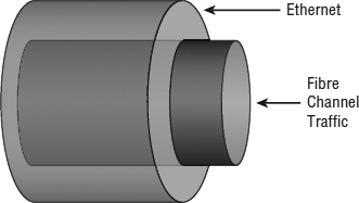
Used together, these three protocols allow Fibre Channel frames to be encapsulated into Ethernet frames, as illustrated in Figure 6.11, and transmitted in a lossless manner. Thus, FCoE uses whatever physical cable plant that 10 Gb Ethernet uses. Today, 10 GbE connectivity is generally optical (same cables as Fibre Channel) and Twinax (which is a pair of coaxial copper cables), InfiniBand-like CX cables, and some emerging 10 Gb unshielded twisted pair (UTP) use cases via the new 10GBase-T standard. Each has its specific distance-based use cases and varying interface cost, size, and power consumption.
FIGURE 6.11 FCoE simply encapsulates Fibre Channel frames into Ethernet frames for transmission over a lossless Ethernet transport.
WHAT ABOUT DATACENTER ETHERNET OR CONVERGED ENHANCED ETHERNET?
Datacenter Ethernet (DCE) and Converged Enhanced Ethernet (CEE) are prestandard terms used to describe a lossless Ethernet network. DCE describes Cisco's prestandard implementation of the DCB standards; CEE was a multivendor effort of the same nature.
Because FCoE uses Ethernet, why use FCoE instead of NFS or iSCSI over 10 Gb Ethernet? The answer is usually driven by the following two factors:
- There are existing infrastructure, processes, and tools in large enterprises that are designed for Fibre Channel, and they expect WWN addressing, not IP addresses. This provides an option for a converged network and greater efficiency, without a “rip and replace” model. In fact, early prestandard FCoE implementations did not include elements required to cross multiple Ethernet switches. These elements, part of something called FCoE Initialization Protocol (FIP), are part of the official FC-BB-5 standard and are required in order to comply with the final standard. This means that most FCoE switches in use today function as FCoE/LAN/Fibre Channel bridges. This makes them excellent choices to integrate and extend existing 10 GbE/1 GbE LANs and Fibre Channel SAN networks. The largest cost savings, power savings, cable and port reduction, and impact on management simplification are on this layer from the ESXi host to the first switch.
- Certain applications require a lossless, extremely low-latency transport network model—something that cannot be achieved using a transport where dropped frames are normal and long-window TCP retransmit mechanisms are the protection mechanism. Now, this is a very high-end set of applications, and those historically were not virtualized. However, in the era of vSphere 5.5, the goal is to virtualize every workload, so I/O models that can deliver those performance envelopes while still supporting a converged network become more important.
In practice, the debate of iSCSI versus FCoE versus NFS on 10 Gb Ethernet infrastructure is not material. All FCoE adapters are converged adapters, referred to as converged network adapters (CNAs). They support native 10 GbE (and therefore also NFS and iSCSI) as well as FCoE simultaneously, and they appear in the ESXi host as multiple 10 GbE network adapters and multiple Fibre Channel adapters. If you have FCoE support, in effect you have it all. All protocol options are yours.
A list of FCoE CNAs supported by vSphere can be found in the I/O section of the VMware compatibility guide.
UNDERSTANDING ISCSI
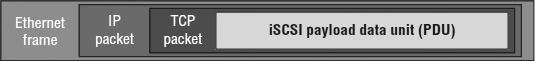
iSCSI brings the idea of a block storage SAN to customers with no Fibre Channel infrastructure. iSCSI is an Internet Engineering Task Force (IETF) standard for encapsulating SCSI control and data in TCP/IP packets, which in turn are encapsulated in Ethernet frames. Figure 6.12 shows how iSCSI is encapsulated in TCP/IP and Ethernet frames. TCP retransmission is used to handle dropped Ethernet frames or significant transmission errors. Storage traffic can be intense relative to most LAN traffic. This makes it important that you minimize retransmits, minimize dropped frames, and ensure that you have “bet-the-business” Ethernet infrastructure when using iSCSI.
FIGURE 6.12 Using iSCSI, SCSI control and data are encapsulated in both TCP/IP and Ethernet frames.
Although Fibre Channel is often viewed as having higher performance than iSCSI, in many cases iSCSI can more than meet the requirements for many customers, and a carefully planned and scaled-up iSCSI infrastructure can, for the most part, match the performance of a moderate Fibre Channel SAN.
Also, iSCSI and Fibre Channel SANs are roughly comparable in complexity and share many of the same core concepts. Arguably, getting the first iSCSI LUN visible to an ESXi host is simpler than getting the first Fibre Channel LUN visible for people with expertise with Ethernet but not Fibre Channel because understanding worldwide names and zoning is not needed. In practice, designing a scalable, robust iSCSI network requires the same degree of diligence that is applied to Fibre Channel. You should use VLAN (or physical) isolation techniques similarly to Fibre Channel zoning, and you need to scale up connections to achieve comparable bandwidth. Look at Figure 6.13, and compare it to the switched Fibre Channel network diagram in Figure 6.8.
FIGURE 6.13 Notice how the topology of an iSCSI SAN is the same as a switched Fibre Channel SAN.
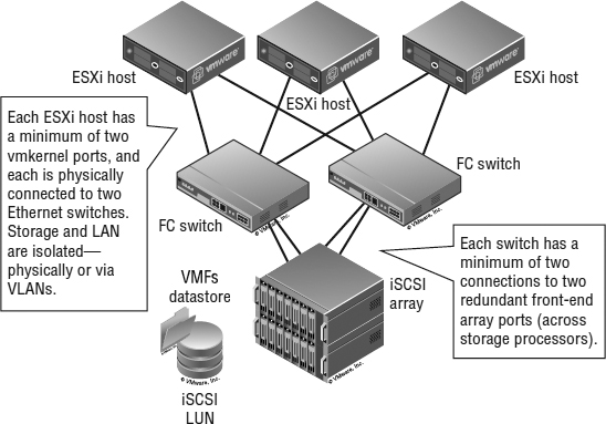
Each ESXi host has a minimum of two VMkernel ports, and each is physically connected to two Ethernet switches. (Recall from Chapter 5, “Creating and Configuring Virtual Networks,” that VMkernel ports are used by the hypervisor for network traffic such as IP-based storage traffic, like iSCSI or NFS.) Storage and LAN are isolated—physically or via VLANs. Each switch has a minimum of two connections to two redundant front-end array network interfaces (across storage processors).
The one additional concept to focus on with iSCSI is the concept of fan-in ratio. This applies to all shared storage networks, including Fibre Channel, but the effect is often most pronounced with Gigabit Ethernet (GbE) networks. Across all shared networks, there is almost always a higher amount of bandwidth available across all the host nodes than there is on the egress of the switches and front-end connectivity of the array. It's important to remember that the host bandwidth is gated by congestion wherever it occurs. Don't minimize the array port-to-switch configuration. If you connect only four GbE interfaces on your array and you have 100 hosts with two GbE interfaces each, then expect contention, because your fan-in ratio is too large.
Also, when iSCSI and iSCSI SANs are examined, many core ideas are similar to Fibre Channel and Fibre Channel SANs, but in some cases there are material differences. Let's look at the terminology:
iSCSI Initiator An iSCSI initiator is a logical host-side device that serves the same function as a physical host bus adapter in Fibre Channel/FCoE or SCSI/SAS. iSCSI initiators can be software initiators (which use host CPU cycles to load/unload SCSI payloads into standard TCP/IP packets and perform error checking) or hardware initiators (the iSCSI equivalent of a Fibre Channel HBA or FCoE CNA). Examples of software initiators that are pertinent to vSphere administrators are the native ESXi software initiator and the guest software initiators available in Windows XP and later and in most current Linux distributions. Examples of iSCSI hardware initiators are add-in cards like the QLogic QLA 405x and QLE 406x host bus adapters. These cards perform all the iSCSI functions in hardware. An iSCSI initiator is identified by an iSCSI qualified name (referred to as an IQN). An iSCSI initiator uses an iSCSI network portal that consists of one or more IP addresses. An iSCSI initiator “logs in” to an iSCSI target.
iSCSI Target An iSCSI target is a logical target-side device that serves the same function as a target in Fibre Channel SANs. It is the device that hosts iSCSI LUNs and masks to specific iSCSI initiators. Different arrays use iSCSI targets differently—some use hardware, some use software implementations—but largely this is unimportant. More important is that an iSCSI target doesn't necessarily map to a physical port as is the case with Fibre Channel; each array does this differently. Some have one iSCSI target per physical Ethernet port; some have one iSCSI target per iSCSI LUN, which is visible across multiple physical ports; and some have logical iSCSI targets that map to physical ports and LUNs in any relationship the administrator configures within the array. An iSCSI target is identified by an iSCSI qualified name (an IQN). An iSCSI target uses an iSCSI network portal that consists of one or more IP addresses.
iSCSI Logical Unit An iSCSI LUN is a LUN hosted by an iSCSI target. There can be one or more LUNs behind a single iSCSI target.
iSCSI Network Portal An iSCSI network portal is one or more IP addresses that are used by an iSCSI initiator or iSCSI target.
iSCSI Qualified Name An iSCSI qualified name (IQN) serves the purpose of the WWN in Fibre Channel SANs; it is the unique identifier for an iSCSI initiator, target, or LUN. The format of the IQN is based on the iSCSI IETF standard.
Challenge Authentication Protocol CHAP is a widely used basic authentication protocol, where a password exchange is used to authenticate the source or target of communication. Unidirectional CHAP is one-way; the source authenticates to the destination, or, in the case of iSCSI, the iSCSI initiator authenticates to the iSCSI target. Bidirectional CHAP is two-way; the iSCSI initiator authenticates to the iSCSI target, and vice versa, before communication is established. Although Fibre Channel SANs are viewed as intrinsically secure because they are physically isolated from the Ethernet network, and although initiators not zoned to targets cannot communicate, this is not by definition true of iSCSI. With iSCSI, it is possible (but not recommended) to use the same Ethernet segment as general LAN traffic, and there is no intrinsic zoning model. Because the storage and general networking traffic could share networking infrastructure, CHAP is an optional mechanism to authenticate the source and destination of iSCSI traffic for some additional security. In practice, Fibre Channel and iSCSI SANs have the same security and same degree of isolation (logical or physical).
IP Security IPsec is an IETF standard that uses public-key encryption techniques to secure the iSCSI payloads so that they are not susceptible to man-in-the-middle security attacks. Like CHAP for authentication, this higher level of optional security is part of the iSCSI standards because it is possible (but not recommended) to use a general-purpose IP network for iSCSI transport—and in these cases, not encrypting data exposes a security risk (for example, a man-in-the-middle attack could determine data on a host it can't authenticate to by simply reconstructing the data from the iSCSI packets). IPsec is relatively rarely used because it has a heavy CPU impact on the initiator and the target.
Static/Dynamic Discovery iSCSI uses a method of discovery where the iSCSI initiator can query an iSCSI target for the available LUNs. Static discovery involves a manual configuration, whereas dynamic discovery issues an iSCSI-standard SendTargets command to one of the iSCSI targets on the array. This target then reports all the available targets and LUNs to that particular initiator.
iSCSI Naming Service The iSCSI Naming Service (iSNS) is analogous to the Domain Name System (DNS); it's where an iSNS server stores all the available iSCSI targets for a very large iSCSI deployment. iSNS is rarely used.
Figure 6.14 shows the key iSCSI elements in an example logical diagram. This diagram shows iSCSI in the broadest sense.
In general, the iSCSI session can be multiple TCP connections, called Multiple Connections Per Session. Note that this cannot be done in VMware. An iSCSI initiator and iSCSI target can communicate on an iSCSI network portal that can consist of one or more IP addresses. The concept of network portals is done differently on each array; some arrays always have one IP address per target port, while some arrays use network portals extensively. The iSCSI initiator logs into the iSCSI target, creating an iSCSI session. You can have many iSCSI sessions for a single target, and each session can have multiple TCP connections (Multiple Connections Per Session, which isn't currently supported by vSphere). There can be varied numbers of iSCSI LUNs behind an iSCSI target—many or just one. Every array does this differently. We'll discuss the particulars of the vSphere software iSCSI initiator implementation in detail in the section “Adding a LUN via iSCSI.”
What about the debate regarding hardware iSCSI initiators (iSCSI HBAs) versus software iSCSI initiators? Figure 6.15 shows the differences among software iSCSI on generic network interfaces, network interfaces that do TCP/IP offload, and full iSCSI HBAs. Clearly there are more things the ESXi host needs to process with software iSCSI initiators, but the additional CPU is relatively light. Fully saturating several GbE links will use only roughly one core of a modern CPU, and the cost of iSCSI HBAs is usually less than the cost of slightly more CPU. Keep the CPU overhead in mind as you craft your storage design, but don't let it be your sole criterion.
FIGURE 6.14 The iSCSI IETF standard has several different elements.
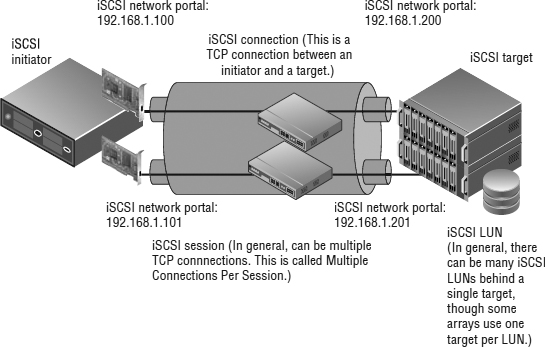
FIGURE 6.15 Some parts of the stack are handled by the adapter card versus the ESXi host CPU in various implementations.
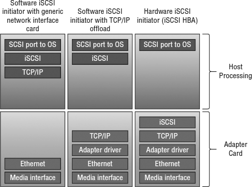
Also note the difference between a dependent hardware iSCSI adapter and an independent hardware iSCSI adapter. As the name suggests, the former depends on vSphere networking and iSCSI configuration, whereas the latter uses its own networking and iSCSI configuration.
Prior to vSphere 5.0, one thing that remained the exclusive domain of the iSCSI HBAs was booting from an iSCSI SAN. From version 5.0, vSphere includes support for iSCSI Boot Firmware Table (iBFT), a mechanism that enables booting from iSCSI SAN with a software iSCSI initiator. You must have appropriate support for iBFT in the hardware. One might argue that using Auto Deploy would provide much of the same benefit as booting from an iSCSI SAN, but each approach has its advantages and disadvantages.
iSCSI is the last of the block-based shared storage options available in vSphere; now we move on to the Network File System (NFS), the only NAS protocol that vSphere supports.
JUMBO FRAMES ARE SUPPORTED
VMware ESXi does support jumbo frames for all VMkernel traffic, including both iSCSI and NFS, and they should be used when needed. However, it is then critical to configure a consistent, larger maximum transfer unit (MTU) size on all devices in all the possible networking paths; otherwise, Ethernet frame fragmentation will cause communication problems. Depending on the network hardware and traffic type, jumbo frames may or may not yield significant benefits. As always, you will need to weigh the benefits against the operational overhead of supporting this configuration.
UNDERSTANDING THE NETWORK FILE SYSTEM
NFS protocol is a standard originally developed by Sun Microsystems to enable remote systems to access a file system on another host as if it were locally attached. vSphere implements a client compliant with NFSv3 using TCP.
When NFS datastores are used by vSphere, no local file system (such as VMFS) is used. The file system is on the remote NFS server. This means that NFS datastores need to handle the same access control and file-locking requirements that vSphere delivers on block storage using the vSphere Virtual Machine File System, or VMFS (we'll describe VMFS in more detail later in this chapter in the section “Examining the vSphere Virtual Machine File System”). NFS servers accomplish this through traditional NFS file locks.
The movement of the file system from the ESXi host to the NFS server also means that you don't need to handle zoning/masking tasks. This makes an NFS datastore one of the easiest storage options to simply get up and running. On the other hand, it also means that all of the high availability and multipathing functionality that is normally part of a Fibre Channel, FCoE, or iSCSI storage stack is replaced by the networking stack. We'll discuss the implications of this in the section titled “Crafting a Highly Available NFS Design.”
Figure 6.16 shows the topology of an NFS configuration. Note the similarities to the topologies in Figure 6.8 and Figure 6.13.
Technically, any NFS server that complies with NFSv3 over TCP will work with vSphere (vSphere does not support NFS over UDP), but similar to the considerations for Fibre Channel and iSCSI, the infrastructure needs to support your entire vSphere environment. Therefore, we recommend you use only NFS servers that are explicitly on the VMware HCL.
Using NFS datastores moves the elements of storage design associated with LUNs from the ESXi hosts to the NFS server. Instead of exposing block storage—which uses the RAID techniques described earlier for data protection—and allowing the ESXi hosts to create a file system (VMFS) on those block devices, the NFS server uses its block storage—protected using RAID—and creates its own file systems on that block storage. These file systems are then exported via NFS and mounted on your ESXi hosts.
FIGURE 6.16 The topology of an NFS configuration is similar to iSCSI from a connectivity standpoint but very different from a configuration standpoint.

In the early days of using NFS with VMware, NFS was categorized as being a lower-performance option for use with ISOs and templates but not production VMs. If production VMs were used on NFS datastores, the historical recommendation would have been to relocate the VM swap to block storage. Although it is true that NAS and block architectures are different and, likewise, their scaling models and bottlenecks are generally different, this perception is mostly rooted in how people have used NAS historically.
The reality is that it's absolutely possible to build an enterprise-class NAS infrastructure. NFS datastores can support a broad range of virtualized workloads and do not require you to relocate the VM swap. However, in cases where NFS will be supporting a broad set of production VM workloads, you will need to pay attention to the NFS server backend design and network infrastructure. You need to apply the same degree of care to bet-the-business NAS as you would if you were using block storage via Fibre Channel, FCoE, or iSCSI. With vSphere, your NFS server isn't being used as a traditional file server, where performance and availability requirements are relatively low. Rather, it's being used as an NFS server supporting a mission-critical application—in this case the vSphere environment and all the VMs on those NFS datastores.
We mentioned previously that vSphere implements an NFSv3 client using TCP. This is important to note because it directly impacts your connectivity options. Each NFS datastore uses two TCP sessions to the NFS server: one for NFS control traffic and the other for NFS data traffic. In effect, this means that the vast majority of the NFS traffic for a single datastore will use a single TCP session. Consequently, this means that link aggregation (which works on a per-flow basis from one source to one target) will use only one Ethernet link per datastore, regardless of how many links are included in the link aggregation group. To use the aggregate throughput of multiple Ethernet interfaces, you need multiple datastores, and no single datastore will be able to use more than one link's worth of bandwidth. The approach available to iSCSI (multiple iSCSI sessions per iSCSI target) is not available in the NFS use case. We'll discuss techniques for designing high-performance NFS datastores in the section titled “Crafting a Highly Available NFS Design.”
As in the previous sections that covered the common storage array architectures, the protocol choices available to the vSphere administrator are broad. You can make most vSphere deployments work well on all protocols, and each has advantages and disadvantages. The key is to understand and determine what will work best for you. In the following section, we'll summarize how to make these basic storage choices.
Making Basic Storage Choices
Most vSphere workloads can be met by midrange array architectures (regardless of active-active, active-passive, asymmetrical, or virtual port design). Use enterprise array designs when mission-critical and very large-scale virtual datacenter workloads demand uncompromising availability and performance linearity.
As shown in Table 6.1, each storage choice can support most use cases. It's not about one versus the other but rather about understanding and leveraging their differences and applying them to deliver maximum flexibility.
TABLE 6.1: Storage choices
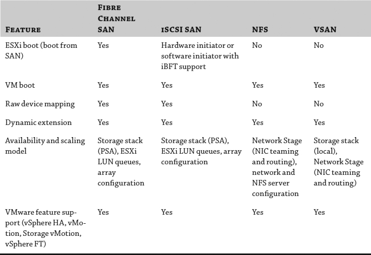
Picking a protocol type has historically been focused on the following criteria:
vSphere Feature Support Although major VMware features such as vSphere HA and vMotion initially required VMFS, they are now supported on all storage types, including raw device mappings (RDMs) and NFS datastores. vSphere feature support is generally not a protocol-selection criterion, and there are only a few features that lag on RDMs and NFS, such as native vSphere snapshots on physical compatibility mode RDMs or the ability to create RDMs on NFS.
Storage Capacity Efficiency Thin provisioning behavior at the vSphere layer, universally and properly applied, drives a very high efficiency, regardless of protocol choice. Applying thin provisioning at the storage array (on both block and NFS objects) delivers a higher overall efficiency than applying it only at the virtualization layer. Emerging techniques for extra array capacity efficiency (such as detecting and reducing storage consumed when there is information in common using compression and data deduplication) are currently most effectively used on NFS datastores but are expanding to include block use cases. One common error is to look at storage capacity (GB) as the sole vector of efficiency—in many cases, the performance envelope requires a fixed number of spindles even with advanced caching techniques. Often in these cases, efficiency is measured in spindle density, not in GB. For most vSphere customers, efficiency tends to be a function of operational process rather than protocol or platform choice.
Performance Many vSphere customers see similar performance regardless of a given protocol choice. Properly designed iSCSI and NFS over Gigabit Ethernet can support very large VMware deployments, particularly with small-block (4 KB–64 KB) I/O patterns that characterize most general Windows workloads and don't need more than roughly 80 MBps of 100 percent read or write I/O bandwidth or 160 MBps of mixed I/O bandwidth. This difference in the throughput limit is due to the 1 Gbps/2 Gbps bidirectional nature of 1GbE—pure read or pure write workloads are unidirectional, but mixed workloads are bidirectional.
Fibre Channel (and by extension, FCoE) generally delivers a better performance envelope with very large-block I/O (VMs supporting DSS database workloads or SharePoint), which tends to demand a high degree of throughput. Less important generally but still important for some workloads, Fibre Channel delivers a lower-latency model and also tends to have a faster failover behavior because iSCSI and NFS always depend on some degree of TCP retransmission for loss and, in some iSCSI cases, ARP—all of which drive failover handling into tens of seconds versus seconds with Fibre Channel or FCoE. Load balancing and scale-out with IP storage using multiple Gigabit Ethernet links with IP storage can work for iSCSI to drive up throughput. Link aggregation techniques can help, but they work only when you have many TCP sessions. Because the NFS client in vSphere uses a single TCP session for data transmission, link aggregation won't improve the throughput of individual NFS datastores. Broad availability of 10 Gb Ethernet brings higher-throughput options to NFS datastores.
You can make every protocol configuration work in almost all use cases; the key is in the details (covered in this chapter). In practice, the most important thing is what you know and feel comfortable with.
The most flexible vSphere configurations tend to use a combination of both VMFS (which requires block storage) and NFS datastores (which require NAS), as well as RDMs on a selective basis (block storage).
The choice of which block protocol should be used to support the VMFS and RDM use cases depends on the enterprise more than the technologies and tends to follow this pattern:
- iSCSI for customers who have never used and have no existing Fibre Channel SAN infrastructure
- Fibre Channel for those with existing Fibre Channel SAN infrastructure that meets their needs
- FCoE for those upgrading existing Fibre Channel SAN infrastructure
vSphere can be applied to a very broad set of use cases—from the desktop/laptop to the server and on the server workloads—ranging from test and development to heavy workloads and mission-critical applications. A simple one-size-fits-all model can work, but only for the simplest deployments. The advantage of vSphere is that all protocols and all models are supported. Becoming fixated on one model means that not everything is virtualized that can be and the enterprise isn't as flexible and efficient as it can be.
Now that you've learned about the basic principles of shared storage and determined how to make the basic storage choices for your environment, it's time to see how these are applied in vSphere.
Implementing vSphere Storage Fundamentals
This part of the chapter examines how the shared storage technologies covered previously are applied in vSphere. We will cover these elements in a logical sequence, starting with core vSphere storage concepts. Next, we'll cover the storage options in vSphere for datastores to contain groups of VMs (VMFS datastores and NFS datastores). We'll follow that discussion with options for presenting disk devices directly into VMs (raw device mappings). Finally, we'll examine VM-level storage configuration details.
Reviewing Core vSphere Storage Concepts
One of the core concepts of virtualization is encapsulation. What used to be a physical system is encapsulated by vSphere, resulting in VMs that are represented by a set of files. Chapter 9, “Creating and Managing Virtual Machines,” provides more detail on the specific files that compose a VM and their purpose. For reasons we've described already, these VM files reside on the shared storage infrastructure (with the exception of a raw device mapping, or RDM, which we'll discuss shortly).
In general, vSphere uses a shared-everything storage model. All ESXi hosts in a vSphere environment use commonly accessed storage objects using block storage protocols (Fibre Channel, FCoE, or iSCSI, in which case the storage objects are LUNs) or network attached storage protocols (NFS, in which case the storage objects are NFS exports). Depending on the environment, these storage objects will be exposed to the majority of your ESXi hosts, although not necessarily to all ESXi hosts in the environment. In Chapter 7, we'll again review the concept of a cluster, which is a key part of features like vSphere HA and vSphere DRS. Within a cluster, you'll want to ensure that all ESXi hosts have visibility and access to the same set of storage objects.
Before we get into the details of how to configure the various storage objects in vSphere, we need to first review some core vSphere storage technologies, concepts, and terminology. This information will provide a foundation upon which we will build later in the chapter. We'll start with a look at the vSphere Virtual Machine File System, a key technology found in practically every vSphere deployment.
EXAMINING THE VSPHERE VIRTUAL MACHINE FILE SYSTEM
The vSphere Virtual Machine File System (VMFS) is a common configuration option for many vSphere deployments. It's similar to NTFS for Windows Server and ext3 for Linux. Like these file systems, it is native; it's included with vSphere and operates on top of block storage objects. If you're leveraging any form of block storage, you're using VMFS.
The purpose of VMFS is to simplify the storage environment. It would clearly be difficult to scale a virtual environment if each VM directly accessed its own storage rather than storing the set of files on a shared volume. VMFS creates a shared storage pool that is used for one or more VMs.
While similar to NTFS and ext3, VMFS differs from these common file systems in several important ways:
- It was designed to be a clustered file system from its inception; neither NTFS nor ext3 is a clustered file system. Unlike many clustered file systems, it is simple and easy to use.
- VMFS's simplicity is derived from its simple and transparent distributed locking mechanism. This is generally much simpler than traditional clustered file systems with network cluster lock managers.
- VMFS enables simple direct-to-disk, steady-state I/O that results in high throughput at a low CPU overhead for the ESXi hosts.
- Locking is handled using metadata in a hidden section of the file system, as illustrated in Figure 6.17. The metadata portion of the file system contains critical information in the form of on-disk lock structures (files), such as which ESXi host is the current owner of a given VM, ensuring that there is no contention or corruption of the VM.
- Depending on the storage array's support for VAAI, when these on-disk lock structures are updated, the ESXi host performing the update momentarily locks the LUN using a nonpersistent SCSI lock (SCSI Reserve/Reset commands). This operation is completely transparent to the vSphere administrator.
- These metadata updates do not occur during normal read/write I/O operations and do not represent a fundamental scaling limit when compared with more traditional file systems.
- During the metadata updates, there is minimal impact to the production I/O (covered in a VMware white paper at www.vmware.com/resources/techresources/1059). This impact is negligible to the ESXi host holding the SCSI lock but more pronounced on the other hosts accessing the same VMFS datastore.
- These metadata updates include, but are not limited to the following:
FIGURE 6.17 VMFS stores metadata in a hidden area of the first extent.
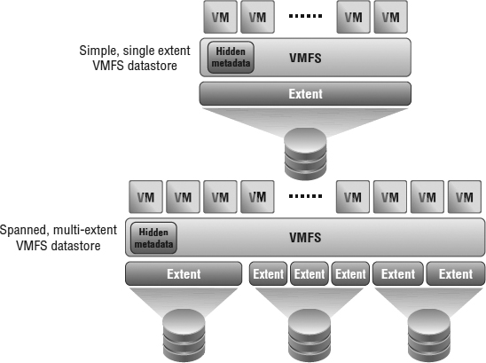
VSPHERE 5.5 AND SCSI-3 DEPENDENCY
In vSphere 5.5, like previous vSphere versions, only SCSI-3–compliant block storage objects are supported. Most major storage arrays have, or can be upgraded via their array software to, full SCSI-3 support, but check with your storage vendor before upgrading. If your storage array doesn't support SCSI-3, the storage details shown on the Configuration tab for the vSphere host will not display correctly.
In spite of this requirement, vSphere still uses SCSI-2 reservations for general ESXi-level SCSI reservations (not to be confused with guest-level reservations). This is important for Asymmetrical Logical Unit Access (ALUA) support, covered in the section “Reviewing Multipathing.”
Earlier versions of vSphere exclusively used VMFS version 3 (VMFS-3), and vSphere 5.0, 5.1, and 5.5 continue to provide support for VMFS-3. In addition to supporting VMFS-3, vSphere 5.0 introduced VMFS version 5 (VMFS-5) with further enhancements in vSphere 5.5. Only hosts running ESXi 5.0 or later support VMFS-5; hosts running ESX/ESXi 4.x will not be able to see or access VMFS-5 datastores. VMFS-5 offers a number of advantages:
- VMFS-5 datastores can now grow up to 64 TB in size using only a single extent. Datastores built on multiple extents are still limited to 64 TB as well.
- VMFS-5 datastores use a single block size of 1 MB, but you can now create files of up to 62 TB on VMFS-5 datastores.
- VMFS-5 uses a more efficient sub-block allocation size of only 8 KB, compared to 64 KB for VMFS-3.
- VMFS-5 lets you create virtual-mode RDMs for devices up to 62 TB in size. (VMFS-3 limits RDMs to 2 TB in size. We'll cover RDMs later in the section “Working with Raw Device Mappings.”)
Even better than the improvements in VMFS-5 is the fact that you can upgrade VMFS-3 datastores to VMFS-5 in place and online—without any disruption to the VMs running on that datastore. You're also not required to upgrade VMFS-3 datastores to VMFS-5, which further simplifies the migration from earlier versions.
Later in this chapter in the section “Working with VMFS Datastores,” we'll provide more details on how to create, expand, delete, and upgrade VMFS datastores.
Closely related to VMFS is the idea of multipathing, a topic that we will discuss in the next section.
REVIEWING MULTIPATHING
Multipathing is the term used to describe how a host, such as an ESXi host, manages storage devices that have multiple ways (or paths) to access them. Multipathing is extremely common in Fibre Channel and FCoE environments and is also found in iSCSI environments. We won't go so far as to say that multipathing is strictly for block-based storage environments, but we will say that multipathing for NFS is generally handled much differently than for block storage.
In vSphere 4, VMware and VMware technology partners spent considerable effort overhauling how the elements of the vSphere storage stack that deal with multipathing work. This architecture, known as the Pluggable Storage Architecture (PSA), is still present in vSphere 5.5 as well. Figure 6.18 shows an overview of the PSA.
FIGURE 6.18 vSphere's Pluggable Storage Architecture is highly modular and extensible.
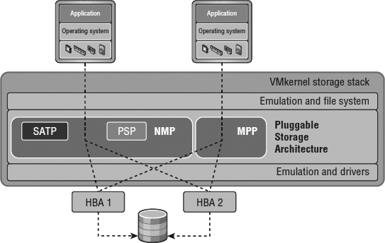
One of the key goals in the development of the PSA was to make vSphere multipathing much more flexible. Pre–vSphere 4 versions of VMware ESX/ESXi had a rigid set of lists that determined failover policy and multipathing policy, and this architecture was updated only with major VMware releases. With the PSA's modular architecture, vSphere administrators have a much more flexible approach.
Four different modules compose the PSA:
- Native multipathing plug-in (NMP)
- Storage array type plug-in (SATP)
- Path selection plug-in (PSP)
- Multipathing plug-in (MPP)
Any given ESXi host can have multiple modules in use at any point and can be connected to multiple arrays, and you can configure the combination of modules used (an NMP/SATP/PSP combination or an MPP) on a LUN-by-LUN basis.
Let's see how they work together.
Understanding the NMP Module
The NMP module handles overall MPIO (multipath I/O) behavior and array identification. The NMP leverages the SATP and PSP modules and isn't generally configured in any way.
Understanding SATP Modules
SATP modules handle path failover for a given storage array and determine the failover type for a LUN.
vSphere ships with SATPs for a broad set of arrays, with generic SATPs for nonspecified arrays and a local SATP for local storage. The SATP modules contain the rules on how to handle array-specific actions or behavior as well as any specific operations needed to manage array paths. This is part of what makes the NMP modular (unlike the NMP in prior versions); it doesn't need to contain the array-specific logic, and additional modules for new arrays can be added without changing the NMP. Using the SCSI Array ID reported by the array via a SCSI query, the NMP selects the appropriate SATP to use. After that, the SATP monitors, deactivates, and activates paths (and when a manual rescan occurs, detects new paths)—providing information up to the NMP. The SATP also performs array-specific tasks such as activating passive paths on active-passive arrays.
To see what array SATP modules exist, enter the following command from the vCLI (we ran this from the ESXi shell):
esxcli storage nmp satp list
Figure 6.19 shows the results this command returns (note that the default PSP for a given SATP is also shown).
Understanding PSP Modules
The PSP module handles the actual path used for every given I/O.
The NMP assigns a default PSP, which can be overridden manually for every LUN based on the SATP associated with that device. This command (and the output captured in Figure 6.20) shows you the three PSPs vSphere includes by default:
esxcli storage nmp psp list
FIGURE 6.19 Only the SATPs for the arrays to which an ESXi host is connected are loaded.
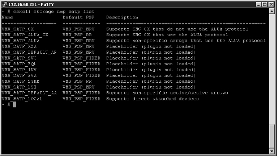
FIGURE 6.20 vSphere ships with three default PSPs.
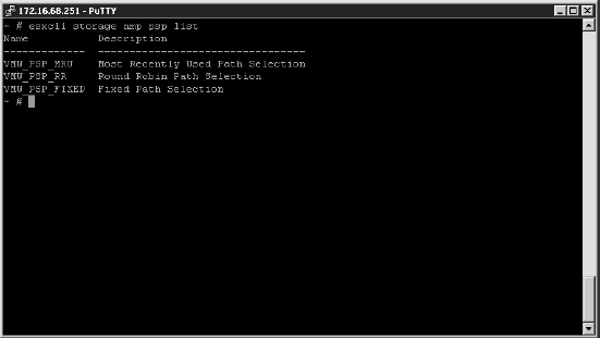
Each of these PSPs performs path selection slightly differently:
- Most Recently Used (noted as VMW_PSP_MRU) selects the path it used most recently. If this path becomes unavailable, the ESXi host switches to an alternative path and continues to use the new path while it is available. This is the default for active-passive array types.
- Fixed (noted as VMW_PSP_FIXED) uses the designated preferred path, if it has been configured. Otherwise, it uses the first working path discovered at system boot time. If the ESXi host cannot use the preferred path, it selects a random alternative available path. The ESXi host automatically reverts to the preferred path as soon as the path becomes available. This is the default for active-active array types (or active-passive arrays that use ALUA with SCSI-2 reservation mechanisms—in these cases, they appear as active-active).
- Round Robin (noted as VMW_PSP_RR) rotates the path selection among all available optimized paths and enables basic load balancing across the paths and fabrics. This is not a weighted algorithm, nor is it responsive to queue depth, but it is a significant improvement. In prior ESXi versions, there was no way to load balance a LUN, and customers needed to statically distribute LUNs across paths, which was a poor proxy for true load balancing.
WHICH PSP IS RIGHT IF YOU'RE USING ALUA?
What do you do if your array can be configured to use ALUA—and therefore could use the Fixed, MRU, or Round Robin policy? See the section “Understanding Midrange and External Enterprise Storage Array Design” for information on ALUA.
The Fixed and MRU path failover policies deliver failover only and work fine with active-active and active-passive designs, regardless of whether ALUA is used. Of course, they both drive workloads down a single path. Ensure that you manually select active I/O paths that are the “good” ports, which are the ones where the port is on the storage processor owning the LUN. You don't want to select the “bad” ports, which are the higher-latency, lower-throughput ones that transit the internal interconnect to get to the LUN.
The out-of-the-box load-balancing policy in vSphere (Round Robin) doesn't use the non-optimized paths (though they are noted as active in the vSphere Web Client). Third-party multipathing plug-ins that are aware of the difference between the asymmetrical path choices can optimize an ALUA configuration.
Perform the following steps to see what SATP (and PSP) is being used for a given LUN in the vSphere Web Client:
- In the vSphere Web Client, navigate to the Hosts And Clusters view.
- Select a host from the list on the left; then select the Manage tab on the right.
- Click the Storage subsection.
- Finally, click the Storage Devices selection on the left.
This opens the Storage Devices area. When a LUN or disk is selected from the list, an SATP will be listed near the bottom, as shown in Figure 6.21.
In this example, the array is an EMC VNX and the generic VMW_SATP_ALUA_CX is selected. The default PSP is Round Robin (VMware). A change in the PSP takes place immediately when you change it. There is no confirmation. Note that the PSP is configurable on a LUN-by-LUN basis.
WHAT IS ALL THE STUFF IN THE STORAGE DEVICE DETAILS LIST?
In the runtime name, the C is the channel identifier, the T is the target identifier, and the L is the LUN.
And that long text string starting with naa? This is the Network Address Authority ID, which is a unique identifier for the target and a LUN. This ID is guaranteed to be persistent through reboots and is used throughout vSphere.
FIGURE 6.21 The SATP for this datastore is VMW_SATP_ALUA_CX, which is the default SATP for EMC VNX arrays.
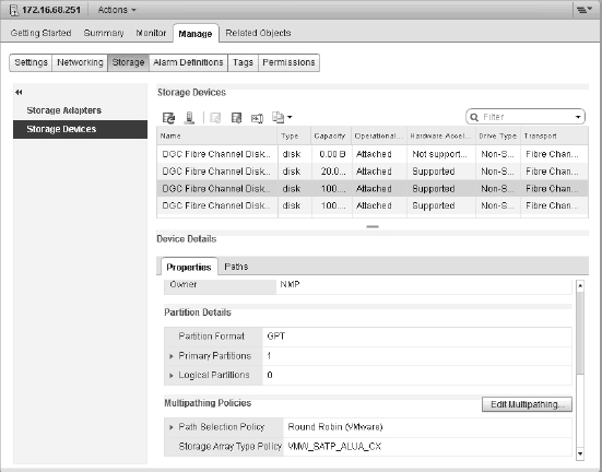
Understanding MPP Modules
The MPP module can add significantly enhanced multipathing to vSphere, and for the given LUNs it supports, it replaces the NMP, SATP, and PSP. The MPP claim policy (the LUNs that it manages) is defined on a LUN-by-LUN and array-by-array basis, and MPPs can coexist with NMP.
Because it replaces the NMP, SATP, and PSP, the MPP can change the path selection normally handled by the PSP. This allows the MPP to provide more sophisticated path selection than the VMware-supplied PSPs can—including selecting by host queue depth and, in some cases, the array target port state. As a result of this more sophisticated path selection, an MPP could offer notable performance increases or other new functionality not present in vSphere by default.
The PSA was written not only to be modular but also to support third-party extensibility; third-party SATPs, PSPs, and MPPs are technically possible. At the time of this writing, only a few MPPs were generally available, though other vendors are likely to create third-party SATPs, PSPs, and potentially full MPPs. Once the MPP is loaded on an ESXi host via the vSphere Web Client's host update tools, all multipathing for LUNs managed by that MPP become fully automated.
AN EXAMPLE OF A THIRD-PARTY MPP
EMC PowerPath/VE is a third-party multipathing plug-in that supports a broad set of EMC and non-EMC array types. PowerPath/VE enhances load balancing, performance, and availability using the following techniques:
- Through active management of intermittent path behavior
- Through more rapid path state detection
- Through automated path discovery behavior without manual rescan
Better performance:
- Through better path selection using weighted algorithms, which is critical in cases where the paths are unequal (ALUA).
- Through monitoring and adjusting the ESXi host queue depth to select the path for a given I/O, shifting the workload from heavily used paths to lightly used paths.
- With some arrays by predictive optimization based on the array port queues. (The array port queues are generally the first point of contention and tend to affect all the ESXi hosts simultaneously; without predictive advance handling, they tend to cause simultaneous path choice across the ESXi cluster.)
Previously in this chapter, in the section on VMFS, we mentioned that one potential advantage to having a VMFS datastore spanned across multiple extents on multiple LUNs would be to increase the parallelism of the LUN queues. In addition, in this section you've heard us mention how a third-party MPP might make multipathing decisions based on host or target queues. Why is queuing so important? We'll review queuing in the next section.
THE IMPORTANCE OF LUN QUEUES
Queues are an important construct in block storage environments (across all protocols, including Fibre Channel, FCoE, and iSCSI). Think of a queue as a line at the supermarket checkout. Queues exist on the server (in this case the ESXi host), generally at both the HBA and LUN levels. They also exist on the storage array. Every array does this differently, but they all have the same concept. Block-centric storage arrays generally have these queues at the target ports, array-wide, at the array LUN levels, and finally at the spindles themselves. File-centric storage arrays generally have queues at the target ports and array-wide, but abstract the array LUN queues because the LUNs actually exist as files in the file system. However, file-centric designs have internal LUN queues underneath the file systems themselves and then ultimately at the spindle level—in other words, it's internal to how the file server accesses its own storage.
The queue depth is a function of how fast things are being loaded into the queue and how fast the queue is being drained. How fast the queue is being drained is a function of the amount of time needed for the array to service the I/O requests. This is called the service time, and in the supermarket checkout it is the speed of the person behind the checkout counter (ergo, the array service time).
CAN I VIEW THE QUEUE?
To determine how many outstanding items are in the queue, use resxtop, press U to get to the storage screen, and look at the QUED column.
The array service time itself is a function of many things, predominantly the workload, then the spindle configuration, then the write cache (for writes only), then the storage processors, and finally, with certain rare workloads, the read caches.
So why is all this important? Well, for most customers it will never come up, and all queuing will be happening behind the scenes. However, for some customers, LUN queues determine whether your VMs are happy or not from a storage performance perspective.
When a queue overflows (either because the storage configuration cannot handle the steady-state workload or because the storage configuration cannot absorb a burst), it causes many upstream effects to slow down the I/O. For IP-focused people, this effect is analogous to TCP windowing, which should be avoided for storage just as queue overflow should be avoided.
You can change the default queue depths for your HBAs and for each LUN/device. (See www.vmware.com for HBA-specific steps.) After changing the queue depths on the HBAs, you need to perform a second step at the VMkernel layer. You must change the amount of outstanding disk requests from the VMs to VMFS to match the HBA setting. You can do this in the ESXi advanced settings, as shown in Figure 6.22 or by using ESXCLI. In general, the default settings for queues and Disk.* are the best. We don't recommend changing these values unless instructed to do so by VMware or your storage vendor.
FIGURE 6.22 It is possible to adjust the advanced properties for advanced use cases, increasing the number of consecutive requests allowed to match adjusted queues.
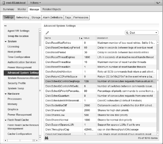
If the queue overflow is not a case of dealing with short bursts but rather that you are under-configured for the steady state workload, making the queues deeper can have a downside: higher latency. Then it overflows anyway. This is the predominant case, so before increasing your LUN queues, check the array service time. If it's taking more than 10 milliseconds to service I/O requests, you need to improve the service time, usually by adding more spindles to the LUN or by moving the LUN to a faster-performing tier.
The last topic we'll cover before moving on to more hands-on topics is the vSphere Storage APIs.
UNCOVERING THE VSPHERE STORAGE APIS
Formerly known as the vStorage APIs, the vSphere Storage APIs aren't necessarily application programming interfaces (APIs) in the truest sense of the word. In some cases, yes, but in other cases, they are simply storage commands that vSphere leverages.
There are several broad families of storage APIs that vSphere offers:
- vSphere Storage APIs for Array Integration
- vSphere APIs for Storage Awareness
- vSphere Storage APIs for Site Recovery
- vSphere Storage APIs for Multipathing
- vSphere Storage APIs for Data Protection
Because of the previous naming convention (vStorage APIs), some of these technologies are more popularly known by their acronyms. Table 6.2 maps the well-known acronyms to their new official names.
TABLE 6.2: vSphere Storage API acronyms
| WELL-KNOWN ACRONYM | OFFICIAL NAME |
| VAAI | vSphere Storage APIs for Array Integration |
| VASA | vSphere APIs for Storage Awareness |
| VADP | vSphere Storage APIs for Data Protection |
In this book, for consistency with the community and the marketplace, we'll use the well-known acronyms to refer to these technologies.
As we mentioned previously, some of these technologies are truly APIs. The Storage APIs for Multipathing are the APIs that VMware partners can use to create third-party MPPs, SATPs, and PSPs for use in the PSA. Similarly, the Storage APIs for Site Recovery encompass the actual programming interfaces that enable array vendors to make their storage arrays work with VMware's Site Recovery Manager product, and the Storage APIs for Data Protection (VADP) are the APIs that third-party companies can use to build virtualization-aware and virtualization-friendly backup solutions.
There are two sets remaining that we haven't yet mentioned, and that's because we'd like to delve into those a bit more deeply. We'll start with the Storage APIs for Array Integration.
Exploring the vSphere Storage APIs for Array Integration
The vSphere Storage APIs for Array Integration (more popularly known as VAAI) were first introduced in vSphere 4.1 as a means of offloading storage-related operations from the ESXi hosts to the storage array. Although VAAI is largely based on SCSI commands ratified by the T10 committee in charge of the SCSI standards, it does require appropriate support from storage vendors, so you'll want to check with your storage vendor to see what is required in order to support VAAI. In addition to the VAAI features introduced in vSphere 4.1 and 5.0, vSphere 5.5 introduces even more storage offloads. Here's a quick rundown of the storage offloads available in vSphere 5.5:
Hardware-Assisted Locking Also called atomic test and set (ATS), this feature supports discrete VM locking without the use of LUN level SCSI reservations. In the section titled “Examining the vSphere Virtual Machine File System,” we briefly described how vSphere uses SCSI reservations when VMFS metadata needs to be updated. Hardware-assisted locking allows for disk locking per sector instead of locking the entire LUN. This offers a dramatic increase in performance when lots of metadata updates are necessary (such as when powering on many VMs at the same time).
Hardware-Accelerated Full Copy Support for hardware-accelerated full copy allows storage arrays to make full copies of data completely internal to the array instead of requiring the ESXi host to read and write the data. This causes a significant reduction in the storage traffic between the host and the array and can reduce the time required to perform operations like cloning VMs or deploying new VMs from templates.
Hardware-Accelerated Block Zeroing Sometimes called write same, this functionality allows storage arrays to zero out large numbers of blocks to provide newly allocated storage without any previously written data. This can speed up operations like creating VMs and formatting virtual disks.
Thin Provisioning vSphere 5.0 added an additional set of hardware offloads around thin provisioning. First, vSphere is thin-provisioning aware, meaning that it will recognize when a LUN presented by an array is thin provisioned. In addition, vSphere 5.0 added and vSphere 5.5 improves on the ability to reclaim dead space (space no longer used) via the T10 UNMAP command; this will help keep space utilization in thin-provisioned environments in check. Finally, vSphere also has support for providing advance warning of thin-provisioned out-of-space conditions and provides better handling for true out-of-space conditions.
STANDARDS-BASED OR PROPRIETARY?
So is the functionality of VAAI standards based or proprietary? Well, the answer is a little of both. In vSphere 4.1, the hardware-accelerated block zeroing was fully T10 compliant, but the hardware-assisted locking and hardware-accelerated full copy were not fully T10 compliant and required specific support from the array vendors. In vSphere 5.5, all three of these features are fully T10 compliant, as is the thin-provisioning support, and will work with any array that is also T10 compliant.
The NAS offloads, however, are not standards based, and will require specific plug-ins from the NAS vendors to take advantage of these offloads.
Like previous versions, vSphere 5.5 includes hardware offloads for NAS:
Reserve Space This functionality lets you create thick-provisioned VMDKs on NFS data-stores, much like what is possible on VMFS datastores.
Full File Clone The Full File Clone functionality allows offline VMDKs to be cloned (copied) by the NAS device.
Lazy File Clone This feature allows NAS devices to create native snapshots for the purpose of space-conservative VMDKs for virtual desktop infrastructure (VDI) environments. It's specifically targeted at emulating the Linked Clone functionality vSphere offers on VMFS datastores.
Extended Statistics When you're leveraging the Lazy File Clone feature, this feature allows more accurate space reporting.
In all cases, support for VAAI requires that the storage vendor's array be fully T10 compliant (for block-level VAAI commands) or support VMware's file-level NAS offloads via a vendor-supplied plug-in. Check with your storage vendor to determine what firmware revisions, software levels, or other requirements are necessary to support VAAI/VAAIv2 with vSphere 5.5.
The vSphere Web Client reports VAAI support, so it's easy to determine if your array has been recognized as VAAI capable by vSphere. Figure 6.23 shows a series of datastores; note the status of the Hardware Acceleration column. You can see that some datastores clearly report Supported in that column.
FIGURE 6.23 If all hardware offload features are supported, the Hardware Acceleration status is listed as Supported.
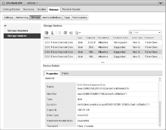
vSphere determines the hardware acceleration status for VMFS datastores and NFS data-stores differently. For VMFS datastores, if at least one of the various SCSI commands is unsupported but others are supported, then the status will be listed as Unknown. If all the commands are unsupported, it will list Not Supported; if all the commands are supported, it will list Supported. You can gather a bit more detail about which commands are supported or not supported using the esxcli command-line utility from the vSphere Management Assistant. Run this command:
esxcli -s vcenter-01 -h esxi-05.lab.local storage core device vaai status get
You'll get output that looks something like Figure 6.24; note that on some LUNS the commands are listed as unsupported. When there is at least one supported and one unsupported per LUN, vSphere reports the status as Unknown.
FIGURE 6.24 The VAAI support detail is more granular when using ESXCLI compared with the Web Client.
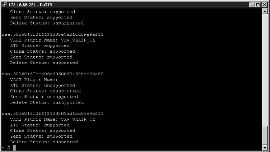
For the inquisitive types who are interested in just a bit more detail on how VAAI works and fits into the vSphere PSA, try running this command from the vSphere Management Assistant:
esxcli -s vcenter-01 -h esxi-05.lab.local storage core claimrules list -c all
The output will look something like Figure 6.25.
FIGURE 6.25 VAAI works hand in hand with claimrules that are used by the PSA for assigning an SATP and PSP for detected storage devices.
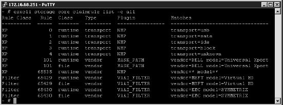
This output shows you that VAAI works in conjunction with the claimrules that the PSA uses when determining the SATP and PSP for a given storage device.
YOU CAN DISABLE VAAI IF NECESSARY
There might be situations where disabling VAAI is required. Some advanced SAN fabric features, for example, aren't currently compatible with VAAI. To disable VAAI, set the value of the following advanced settings to zero:
- /VMFS3/HardwareAcceleratedLocking
- /DataMoverHardwareAcceleratedMove
- /DataMover/HardwareAcceleratedInit
No reboot is necessary for this change to take effect. To re-enable VAAI, change the value for these advanced settings back to 1.
VAAI is not the only mechanism for advanced storage integration with vSphere; with vSphere 5, VMware also introduced the Storage APIs for Storage Awareness. We'll describe those in the next section.
Exploring the vSphere Storage APIs for Storage Awareness
The vSphere APIs for Storage Awareness, more commonly known as VASA (from its previous name, the vStorage APIs for Storage Awareness), enables more advanced out-of-band communication between storage arrays and the virtualization layer. At a high level, VASA operates in the following manner:
- The storage array communicates its capabilities to the VASA provider. These capabilities could be just about anything: replication status, snapshot capabilities, storage tier, drive type, or IOPS capacity. Exactly what capabilities are communicated to the VASA provider are strictly determined by the storage vendor.
- The VASA provider communicates these capabilities to vCenter Server. This allows vSphere administrators to, for the very first time, see storage capabilities within vCenter Server.
To enable this communication, you must have a VASA provider supplied by your storage vendor. This VASA provider might be a separate VM supplied by the storage vendor, or it might be an additional service provided by the software on the array. The one restriction that VMware does place on the VASA provider is that it can't run on the same operating system as vCenter Server. Once you have this VASA provider, you'll then add it to vCenter Server using the Storage Providers area found under vCenter Server ![]() Manage
Manage ![]() Storage Providers, shown in Figure 6.26.
Storage Providers, shown in Figure 6.26.
FIGURE 6.26 The Storage Providers area is where you go to enable communication between the VASA provider and vCenter Server.
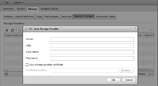
Once the storage provider has been added to vCenter Server, it will communicate storage capabilities up to vCenter Server.
However, the presence of these storage capabilities is only half the picture. The other half of the picture is what the vSphere administrator does with these capabilities: build policy-driven VM storage policies, as we describe in the next section.
EXAMINING POLICY-DRIVEN STORAGE
Working in conjunction with VASA, the principle behind policy-driven storage is simple: Allow vSphere administrators to build VM storage policies that describe the specific storage attributes that a VM requires. Then, allow vSphere administrators to place VMs on datastores that are compliant with that storage policy, thus ensuring that the needs of the VM are properly serviced by the underlying storage. Once a VM is up and running, vCenter monitors and will send an alert if a VM happens to be in breach of the assigned storage policy.
Working with policy-driven storage involves the following three steps:
- Use VASA to populate system storage capabilities and/or create user-defined storage capabilities. System capabilities are automatically propagated to datastores; user-defined capabilities must be manually assigned.
- Create VM storage policies that define the specific features a VM requires from the underlying storage.
- Assign a VM storage policy to a VM and then check its compliance (or noncompliance) with the assigned VM storage policy.
We'll provide the details on how to accomplish step 2 and step 3 later in the section “Creating and Assigning VM Storage Policy.” In the section “Assigning a Storage Capability to a Datastore,” we'll show you how to assign a user-defined storage capability to a datastore.
In the section “Creating and Assigning VM Storage Policies,” we'll show you how to create a VM storage policy and then determine the compliance or noncompliance of a VM with that storage policy.
For now, we'd like to show you how to create a user-defined storage capability. Keep in mind that the bulk of the power of policy-driven storage comes from the interaction with VASA to automatically gather storage capabilities from the underlying array. However, you might find it necessary or useful to define one or more additional storage capabilities that you can use in building your VM storage policies.
Before you can create a custom storage policy, you must have a tag to associate with it. Tags are explained in more detail in Chapter 3, “Installing and Configuring vCenter Server.” The following steps outline how to create tags:
- In the vSphere Web Client, navigate to the Home screen and select Tags from the Navigator list.
- Once in the Tags area, click the New Tag icon.
- Name the tag Gold Storage and select New Category from the drop-down list.
- The New Tag dialog box will expand so you can also create a category. Name this category Storage Types.
- Change Cardinality to Many Tags Per Object.
- Select the check boxes next to Datastore and Datastore Cluster as shown in Figure 6.27.
- Finally, click OK.
FIGURE 6.27 The New Tag dialog box can be expanded to also create a tag category.
- Repeat steps 2 and 3 but select the Storage Types category you just created for additional silver and bronze tags.
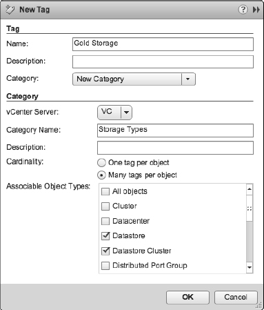
Now that the preparation work is complete, you can perform the following steps to create a user-defined storage capability:
- In the vSphere Web Client, navigate to the Home screen and click the VM Storage Policies icon, shown in Figure 6.28.
FIGURE 6.28 The VM Storage Policies area in the vSphere Web Client is one place to create user-defined storage capabilities. You can also create them from the Datastores And Datastore Clusters view.
- In the VM Storage Policies screen, click the Create A New VM Storage Policy icon.
This will bring up the Create A New VM Storage Policy dialog box.
- Provide a name and description for the new VM storage policy and click Next.
- The Rule-Sets explanation is displayed, Click Next to go to the rule creation page.
- Click the Add Tag-Based Rule button, and choose the tag category and the tag associated with the datastores; then click OK.
Multiple tags can be added to a single rule-set and multiple rule-sets can be added to a storage policy.
- Click Next to finish the rule-set creation and verify the matching resources on the following page.
- Finally, click Next and Finish to exit the Create New VM Storage Policy dialog box.
Figure 6.29 shows a number of a user-defined storage policies.
Any system-provided storage capabilities supplied by VASA will also show up in the Rule-Set page on the Create New VM Storage Policy dialog box. These can be substituted by user-created tags as needed.
You'll come back to the VM Storage Policies area of the vSphere Web Client later in this chapter when we show you how to create a VM storage policy and assign it to a VM.
Now that we've covered some vSphere-specific storage basics, let's move on to working with VMFS datastores.
FIGURE 6.29 VM storage policies can match user-defined tags or vendor-specific capabilities.
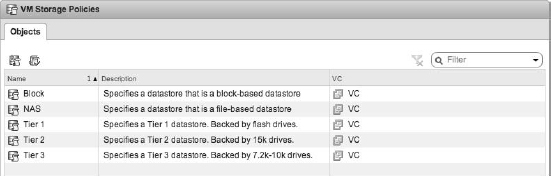
Working with VMFS Datastores
It's time to shift the focus away from concepts and into practice. Next, we'll take a look at working with VMFS datastores. As you have learned, VMFS is the file system that vSphere uses for all block-based storage, so it's common. Working with VMFS datastores will be a daily task that you, as a vSphere administrator, will be responsible for accomplishing.
Let's start with adding a VMFS datastore. Every VMFS datastore is backed by a LUN, so first we'll need to review the process for adding a LUN to your ESXi hosts. The process for adding a LUN will vary based on the block storage protocol, so the next three sections will describe adding a LUN via Fibre Channel, adding a LUN via FCoE (these are essentially the same), and adding a LUN via iSCSI.
ADDING A LUN VIA FIBRE CHANNEL
Adding a LUN to vSphere via Fibre Channel is really more of a task for the storage administrator (who might also be the vSphere administrator in some environments!). As we mentioned previously in the section “Reviewing Fibre Channel,” making a LUN visible over a Fibre Channel SAN involves a few steps, only one of which is done in the vSphere environment:
- Zone the Fibre Channel SAN so that the ESXi host(s) can see the target port(s) on the storage array.
- On the storage array, present the LUN to the ESXi host(s). This procedure varies from vendor to vendor. In a NetApp environment, this involves adding the host's WWNs to an initiator group (or igroup); in an EMC environment, it involves creating a storage group. Refer to your specific storage vendor's instructions.
- Rescan for new storage devices on the ESXi host.
That last step is the only step that involves the vSphere environment. There are two ways to rescan for new storage devices: You can rescan a specific storage adapter, or you can rescan all storage adapters.
Perform the following steps to rescan only a specific storage adapter:
- In the vSphere Web Client, navigate to the Manage tab for a specific ESXi host in the Hosts And Clusters view.
- In the Storage subsection, select Storage Adapters from the left.
This will display the storage adapters recognized in the selected ESXi host.
- Click the Rescan All icon.
- If you want to scan only for new LUNs that have been zoned or presented to the ESXi host, select Scan For New Storage Devices and deselect Scan For New VMFS Volumes.
- If you want to scan only for new VMFS datastores, deselect Scan For New Storage Devices and select Scan For New VMFS Volumes.
- If you want to do both, simply click OK (both are selected by default). You'll see the appropriate tasks appear in the Tasks pane of the vSphere Web Client.
You'll note that two tasks appear in the Recent Tasks pane of the vSphere Web Client: a task for rescanning all the HBAs and a task for rescanning VMFS.
The task for rescanning the HBAs is pretty straightforward; this is a query to the host HBAs to see if new storage is available. If new storage is available to an adapter, it will appear in the details pane of the Storage Adapters area in the vSphere Web Client.
The second task is a bit different. The VMFS rescan is triggered automatically, and it scans available storage devices for an existing VMFS datastore. If it finds an existing VMFS datastore, it will attempt to mount the VMFS datastore and make it available to the ESXi host. Automatically triggering the VMFS rescan simplifies the process of making new VMFS datastores available to ESXi hosts.
In addition to rescanning just all HBAs or CNAs, you can rescan a single storage adapter.
Perform the following steps to rescan a single storage adapter:
- In the vSphere Web Client, navigate to the Manage tab for a specific ESXi host in the Hosts And Clusters view.
- From the Storage subsection, select Storage Adapters on the left.
- Select one of the adapters in the list and then click the Rescan icon above the list (fourth from the left).
YOU CAN ALSO RESCAN AN ENTIRE CLUSTER
If you right-click a cluster object in the Hosts And Clusters view, you can also rescan an entire cluster for new storage objects by clicking All vCenter Actions ![]() Rescan Storage.
Rescan Storage.
Assuming that the zoning of your Fibre Channel SAN is correct and that the storage has been presented to the ESXi host properly, your new LUN should appear in the details pane.
Once the LUN is visible, you're ready to create a new VMFS datastore on it, but before we get to that, we need to cover the processes for adding a LUN via FCoE and via iSCSI.
ADDING A LUN VIA FCOE
The process for adding a LUN via FCoE really depends on one key question: Are you using a CNA where the FCoE is handled in hardware, or are you using vSphere's software-based FCoE initiator?
In previous versions of vSphere, FCoE was supported strictly in hardware, meaning that you could use FCoE only if you had an FCoE CNA installed in your ESXi host. In this configuration, the CNA drivers presented the CNAs to the ESXi host as if they were Fibre Channel HBAs. Therefore, the process of adding a LUN to an ESXi host using hardware-based FCoE was virtually identical to the process we described previously in the section “Adding a LUN via Fibre Channel.” Because it's so similar, we won't repeat those steps here.
However, vSphere 5.0 added the ability to perform FCoE in software via an FCoE software initiator. There is still an element of hardware support required, though; only certain network interface cards that support partial FCoE offload are supported. Refer to the vSphere Compatibility Guide or the vSphere HCL.
Assuming you have a supported NIC, the process for configuring the software FCoE initiator is twofold: Configure the FCoE networking and then activate the software FCoE adapter. In Chapter 5 we explained in much greater detail the networking components, including virtual switches and VMkernel ports, that will be used in the next few sections.
Perform the following steps to configure the networking for software FCoE:
- Log in to the vSphere Web Client, and connect to an ESXi host or to a vCenter Server instance.
- Navigate to the Hosts And Clusters view.
- Select a host from the Navigator panel and then click the Manage tab.
- Select the Network subsection.
- Use the Add Host Networking icon to create a new vSphere Standard Switch with a VMkernel port.
When selecting uplinks for the new vSwitch, be sure to select the NIC that supports partial FCoE offload. You can add multiple NICs to a single vSwitch, or you can add each FCoE offload-capable NIC to a separate vSwitch. However, once you add the NICs to a vSwitch, don't remove them or you'll disrupt the FCoE traffic.
For more information on creating a vSphere Standard Switch, creating a VMkernel port, or selecting uplinks for a vSwitch, refer to Chapter 5.
- Once you've configured the network, select the Storage subsection in the ESXi host
 Manage tab.
(You should still be on this tab after completing the network configuration.)
- Click Add New Storage Adapter icon, select Software FCoE adapter, and click OK.
- On the Add Software FCoE Adapter dialog box, select the appropriate NIC (one that supports partial FCoE offload and that was used as an uplink for the vSwitch you created previously) from the drop-down list of physical adapters.
- Click OK.
OTHER NETWORKING LIMITATIONS FOR SOFTWARE FCOE
Don't move a network adapter port from one vSwitch to another when FCoE traffic is active or you'll run into problems. If you made this change, moving the network adapter port back to the original vSwitch will correct the problem. Reboot your ESXi host if you need to move the network adapter port permanently.
Also, be sure to use a VLAN for FCoE that is not used for any other form of networking on your ESXi host.
Double-check that you've disabled Spanning Tree Protocol (STP) on the ports that will support software FCoE from your ESXi host. Otherwise, the FCoE Initialization Protocol (FIP) exchange might be delayed and cause the software adapter not to function properly.
vSphere will create a new adapter in the list of storage adapters. Once the adapter is created, you can select it to view its properties, such as getting the WWN assigned to the software adapter. You'll use that WWN in the zoning and LUN presentation as described in the section on adding a LUN via Fibre Channel. After you've completed the zoning and LUN presentation, you can rescan the adapter to see the new LUN appear.
The next procedure we'll review is adding a LUN with iSCSI.
ADDING A LUN VIA ISCSI
As with FCoE, the procedure for adding a LUN via iSCSI depends on whether you are using hardware-based iSCSI (using an iSCSI HBA) or leveraging vSphere's software iSCSI initiator.
With a hardware iSCSI solution, the configuration takes place in the iSCSI HBA itself. The instructions for configuring your iSCSI HBA will vary from vendor to vendor; so refer to your specific vendor's documentation on how to configure it to properly connect to your iSCSI SAN. After the iSCSI HBA is configured, then the process for adding a LUN via hardware-based iSCSI is much like the process we described for Fibre Channel, so we won't repeat the steps here.
If you instead choose to use vSphere's software iSCSI initiator, then you can take advantage of iSCSI connectivity without the need for iSCSI hardware installed in your server.
As with the software FCoE adapter, there are a few of different steps involved in setting up the software iSCSI initiator:
- Configure networking for the software iSCSI initiator.
- Activate and configure the software iSCSI initiator.
The following sections describe these steps in more detail.
Configuring Networking for the Software iSCSI Initiator
With iSCSI, although the Ethernet stack can technically be used to perform some multipathing and load balancing, this is not how iSCSI is generally designed. iSCSI uses the same multipath I/O (MPIO) storage framework as Fibre Channel and FCoE SANs. As a result, a specific networking configuration is required to support this framework. In particular, you'll need to configure the networking so that each path through the network uses only a single physical NIC. The MPIO framework can then use each NIC as a path and perform the appropriate multipathing functions. This configuration also allows iSCSI connections to scale across multiple NICs; using Ethernet-based techniques like link aggregation will increase overall throughput but will not increase throughput for any single iSCSI target.
Perform the following steps to configure the virtual networking properly for the software iSCSI initiator:
- In the vSphere Web Client, navigate to the Hosts And Clusters view and select an ESXi host from the inventory panel.
- Select the Manage tab and then click Networking.
- Create a new vSwitch with at least two uplinks. Make sure all uplinks are listed as active NICs in the vSwitch's failover order.
(You can also use a vSphere Distributed Switch, but for simplicity we'll use a vSwitch in this procedure.)
USING SHARED UPLINKS VS. DEDICATED UPLINKS
Generally, a bet-the-business iSCSI configuration will use a dedicated vSwitch with dedicated uplinks. However, if you are using 10 Gigabit Ethernet, you may have only two uplinks. In this case, you will have to use a shared vSwitch and shared uplinks. If at all possible, we recommend configuring Quality of Service on the vSwitch, either by using a vSphere Distributed Switch with Network I/O Control or by using the Cisco Nexus 1000V and QoS. This will help ensure that iSCSI traffic is granted the appropriate network bandwidth so that your storage performance doesn't suffer.
- Create a VMkernel port for use by iSCSI. Configure the VMkernel port to use only one of the available uplinks on the vSwitch.
- Repeat step 4 for each uplink on the vSwitch. Ensure that each VMkernel port is assigned only one active uplink and that no uplinks are shared between VMkernel ports.
Figure 6.30 shows the NIC Teaming tab for an iSCSI VMkernel port; note that only one uplink is listed as an active NIC. All other uplinks must be set to unused in this configuration.
FIGURE 6.30 For proper iSCSI multipathing and scalability, only one uplink can be active for each iSCSI VMkernel port. All others must be set to unused.
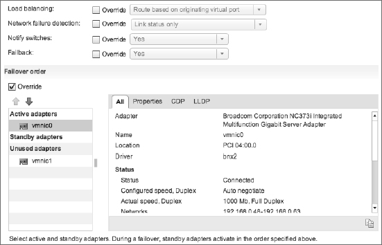
WHAT'S THE MAXIMUM NUMBER OF LINKS THAT YOU CAN USE FOR ISCSI?
You can use the method shown previously to drive I/O down eight separate vmnics. Testing has shown that vSphere can drive nine Gbps of iSCSI throughput through a single ESXi host.
For more information on how to create a vSwitch, assign uplinks, create VMkernel ports, and modify the NIC failover order for a vSwitch or VMkernel port, refer to Chapter 5.
When you finish with the networking configuration, you're ready for the next step.
Activating and Configuring the Software iSCSI Initiator
After configuring the network appropriately for iSCSI, perform these steps to activate and configure the software iSCSI initiator:
- In the vSphere Web Client, navigate to the Hosts And Clusters view and select an ESXi host from the inventory panel.
- Click the Manage tab and select the Storage subsection.
- Click the Add New Storage Adapter icon. From the Add Storage Adapter drop-down, select Software iSCSI Adapter and click OK.
- A dialog box will appear, informing you that a software iSCSI will be added to the list of storage adapters. Click OK.
After a few moments, a new storage adapter under iSCSI Software Adapter will appear, as shown in Figure 6.31.
- Select the new iSCSI adapter.
FIGURE 6.31 This storage adapter is where you will perform all the configuration for the software iSCSI initiator.
- Click the Network Port Binding tab.
- Click the Add button to add a VMkernel port binding.
This will create the link between a VMkernel port used for iSCSI traffic and a physical NIC.
- From the Bind With VMkernel Network Adapter dialog box, select a compliant port group.
A compliant port group is a port group with a VMkernel port configured with only a single physical uplink. Figure 6.32 shows an example of two compliant port groups you could select to bind to the VMkernel network adapter.
FIGURE 6.32 Only compliant port groups will be listed as available to bind with the VMkernel adapter.
Click OK after selecting a compliant port group.
- Repeat step 8 for each VMkernel port and uplink you created previously when configuring the network for iSCSI.
When you've finished, the iSCSI initiator Properties dialog box will look something like Figure 6.33.
- Select the Targets tab and under Dynamic Discovery click Add.
- In the Add Send Target Server dialog box, enter the IP address of the iSCSI target. Click OK when you've finished.
Configuring discovery tells the iSCSI initiator what iSCSI target it should communicate with to get details about storage that is available to it and actually has the iSCSI initiator log in to the target—which makes it known to the iSCSI target. This also populates all the other known iSCSI targets and populates the Static Discovery entries.
- Finally, click the Rescan Adapter icon to discover any new storage devices.
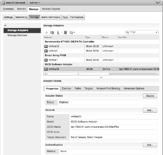
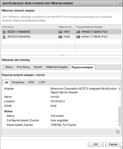
FIGURE 6.33 This configuration allows for robust multipathing and greater bandwidth for iSCSI storage configurations.
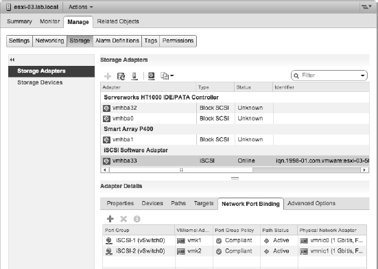
If you've already performed the necessary masking/presentation tasks on the iSCSI array to make LUNs available, then the LUN should now show up in the list of devices on the software iSCSI adapter, and you can use that LUN to create a VMFS datastore. If you haven't already presented the LUN to the ESXi host, you'll need to do so according to your vendor's instructions (every array vendor is different). After the storage is presented to the host, a rescan of the iSCSI adapter—using the procedure we outlined in the section “Adding a LUN via Fibre Channel”—should cause the device to show up.
TROUBLESHOOTING ISCSI LUNS
If you're having a problem getting the iSCSI LUN to show up on your ESXi host, check the following troubleshooting list:
- Can you ping the iSCSI target from the initiator? (Use the Direct Console User Interface [DCUI] to test connectivity from the ESXi host, or enable the ESXi shell and use the vmkping command.)
- Is the physical cabling correct? Are the link lights showing a connected state on the physical interfaces on the ESXi host, the Ethernet switches, and the iSCSI arrays?
- Are your VLANs configured correctly? If you've configured VLANs, have you properly configured the same VLAN on the host, the switch, and the interface(s) that will be used on the array for the iSCSI target?
- Is your IP routing correct and functional? Have you properly configured the IP addresses of the VMkernel port and the interface(s) that will be used on the array for the iSCSI target? Are they on the same subnet? If not, they should be. Although iSCSI can be routed, it's not a good idea because routing adds significant latency and isn't involved in a bet-the-business storage Ethernet network. In addition, it's generally not recommended in vSphere environments.
- Is iSCSI traffic being allowed through any firewalls? If the ping succeeds but subsequently the iSCSI initiator can't log into the iSCSI target, check whether TCP port 3620 is being blocked by a firewall somewhere in the path. Again, the general recommendation is to avoid firewalls in the midst of the iSCSI data path wherever possible to avoid introducing additional latency.
- Is your CHAP configuration correct? Have you correctly configured authentication on both the iSCSI initiator and the iSCSI target?
Now that you have a LUN presented and visible to the ESXi hosts, you can add (or create) a VMFS datastore on that LUN. We'll cover this process in the next section.
CREATING A VMFS DATASTORE
When you have a LUN available to the ESXi hosts, you can create a VMFS datastore.
Before starting this process, you'll want to double-check that the LUN you will be using for the new VMFS datastore is shown under the configuration's Storage Adapters list. (LUNs appear in the bottom of the vSphere Web Client properties pane associated with a storage adapter.) If you've provisioned a LUN that doesn't appear, rescan for new devices.
Perform the following steps to configure a VMFS datastore on an available LUN:
- Launch the vSphere Web Client if it isn't already running, and connect to a vCenter Server instance.
- Navigate to the Hosts And Clusters view, and select an ESXi host from the inventory tree.
- Click the Related Objects tab.
- Click the Create New Datastore icon to launch the New Datastore Wizard.
ANOTHER WAY TO OPEN THE NEW DATASTORE WIZARD
You can also access the New Datastore Wizard by right-clicking a datacenter or ESXi host object in the Navigator and selecting New Datastore from the context menu.
- After clicking Next on the first screen of the New Datastore Wizard, you are prompted for the storage type. Select VMFS, and click Next.
(We'll show you how to use the Add Storage Wizard to create an NFS datastore in the section “Working with NFS Datastores” later in this chapter.)
- Create a name for the new datastore, and then if prompted, select a host that can access the LUN.
We recommend that you use as descriptive a name as possible. You might also consider using a naming scheme that includes an array identifier, a LUN identifier, a protection detail (RAID type and whether it is replicated remotely for disaster recovery purposes), or other key configuration data. Clear datastore naming can help the vSphere administrator later in determining VM placement and can help streamline troubleshooting if a problem arises.
- Select the LUN on which you want to create the new VMFS datastore.
For each visible LUN, you will see the LUN name and identifier information, along with the LUN. Figure 6.34 shows two available LUNs on which to create a VMFS datastore.
FIGURE 6.34 You'll choose from a list of available LUNs when creating a new VMFS datastore.
After you've selected the LUN you want to use, click Next.
- Select whether you'd like to create a VMFS-5 datastore or a VMFS-3 datastore.
We described the differences between VMFS-5 and VMFS-3 in the section titled “Examining the vSphere Virtual Machine File System.” Click Next after selecting a version.
- The next screen, displayed for you in Figure 6.35, shows a summary of the details of the LUN selected and the action that will be taken; if it's a new LUN (no preexisting VMFS partition), the wizard will note that a VMFS partition will be created.
FIGURE 6.35 The Current Partition Layout screen provides information on the partitioning action that will be taken to create a VMFS datastore on the selected LUN.
Click Next to continue.
If the selected LUN has an existing VMFS partition, you will be presented with some different options; see the section “Expanding a VMFS Datastore” for more information.
- If you selected VMFS-3 in step 8, you'll need to select the VMFS allocation size.
For VMFS-5 datastores, you won't need to select a VMFS allocation size (VMFS-5 always uses a 1 MB block size).
Refer back to “Examining the vSphere Virtual Machine File System” for more information on block sizes and their impact.
- For both VMFS-5 and VMFS-3, in the Capacity section you'll specify how you want to utilize the space on the selected LUN.
Generally speaking, you will select Maximize Available Space to use all the space available on the LUN. If, for whatever reason, you can't or don't want to use all of the space available on the LUN, select Custom Space Setting and specify the size of the VMFS datastore you are creating. Click Next when you are ready to proceed.
- At the Ready To Complete screen, double-check all the information. If everything is correct, click Finish; otherwise, use the Back button to go back and make any changes.
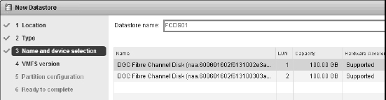
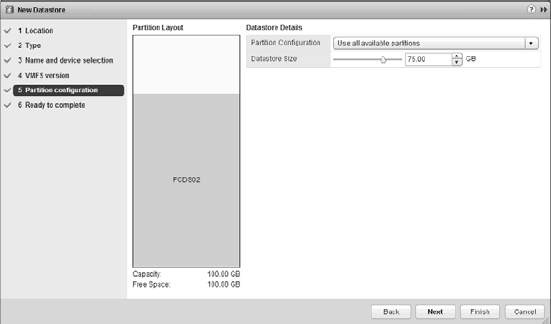
When you click Finish and finish creating the datastore, vSphere will trigger the remaining hosts in the same cluster to rescan for new devices. This ensures that the other hosts in the cluster will also see the LUN and the VMFS datastore on that LUN. You will still need to rescan for devices (using the process in the sections on adding a LUN) for ESXi hosts that are not in the same cluster.
After you've created a VMFS datastore, you may need to complete a few extra tasks. Although these tasks are storage-related, we've included them in other areas of the book. Here's a quick reference to some of the other tasks you might need to perform on a VMFS datastore:
- To enable Storage I/O Control, a mechanism for enforcing prioritized access to storage I/O resources, refer to the section “Controlling Storage I/O Utilization” in Chapter 11.
- To create a datastore cluster to enable Storage DRS, refer to “Introducing and Working with Storage DRS” in Chapter 12, “Balancing Resource Utilization.”
- To create some alarms on this new VMFS datastore, refer to “Using Alarms” in Chapter 13, “Monitoring VMware vSphere Performance.”
Creating new VMFS datastores is not the only way to make additional space available to vSphere for use by VMs. Depending on your configuration, you might be able to expand an existing VMFS datastore, as we'll describe in the next section.
EXPANDING A VMFS DATASTORE
Recall from our previous discussion of VMFS (in the section “Examining the vSphere Virtual Machine File System”) that we mentioned that VMFS supports multiple extents. In previous versions of vSphere, administrators could use multiple extents as a way of getting past the 2 TB limit for VMFS-3 datastores. By combining multiple extents, vSphere administrators could take VMFS-3 datastores up to 64 TB (32 extents of 2 TB each). VMFS-5 eliminates this need because it now supports single-extent VMFS volumes of up to 64 TB in size. However, adding extents is not the only way to expand a VMFS datastore.
If you have a VMFS datastore (either VMFS-3 or VMFS-5), there are two ways of expanding it to make more space available:
- You can dynamically expand the VMFS datastore.
VMFS can be easily and dynamically expanded in vSphere without adding extents, as long as the underlying LUN has more capacity than was configured in the VMFS data-store. Many modern storage arrays have the ability to nondisruptively add capacity to a LUN; when combined with the ability to nondisruptively expand a VMFS volume, this gives you a great deal of flexibility as a vSphere administrator. This is true for both VMFS-3 and VMFS-5.
- You can add an extent.
You can also expand a VMFS datastore by adding an extent. You need to add an extent if the datastore is a VMFS-3 datastore that has already hit its size limit (2 TB minus 512 bytes) or if the underlying LUN on which the datastore resides does not have any additional free space available. This latter condition would apply for VMFS-3 as well as VMFS-5 datastores.
These procedures are extremely similar; many of the steps in both procedures are exactly the same.
Perform these steps to expand a VMFS datastore (either by nondisruptively expanding the datastore on the same LUN or by adding an extent):
- In the vSphere Web Client, navigate to the Hosts inventory list.
- Select a host from the Navigator tree on the left, and then click the Related Objects tab in the content area.
- From the Datastores subsection, select the datastore you wish to expand.
- Click the green Increase Datastore Capacity icon, shown in Figure 6.36. This will open the Increase Datastore Capacity Wizard.
You'll note that this wizard looks similar to the Add Storage Wizard you saw previously when creating a new VMFS datastore.
- If the underlying LUN has free space available, then the Expandable column will report Yes, as shown in Figure 6.37. Select this LUN to nondisruptively expand the VMFS data-store using the free space on the same LUN.
FIGURE 6.36 From the Datastores subsection of the Related Objects tab, you can increase the size of the datastore.
FIGURE 6.37 If the Expandable column reports Yes, the VMFS volume can be expanded into the available free space.
If the underlying LUN has no additional free space available, the Expandable column will report No, and you must expand the VMFS datastore by adding an extent. Select an available LUN.
Click Next when you are ready to proceed.
- If you are expanding the VMFS datastore using free space on the LUN, the Specify Configuration screen will report that the free space will be used to expand the volume.
If you are adding an extent to the VMFS datastore, the Specify Configuration screen will indicate that a new partition will be created.
Click Next to proceed.
- Regardless of the method you're using—expanding into free space on the LUN or adding an extent—if you are expanding a VMFS-3 datastore, you'll note that the block size dropdown list is grayed out. You don't have an option to change the VMFS block size when expanding a VMFS-3 datastore.
- If you didn't want to use or couldn't use all of the free space on the underlying LUN, you could change the capacity from Maximize Available Space to Custom Space Setting and specify the amount. Generally, you will leave the default of Maximize Available Space selected. Click Next.
- Review the summary information, and if everything is correct, click Finish.
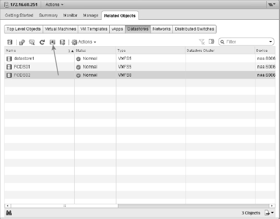
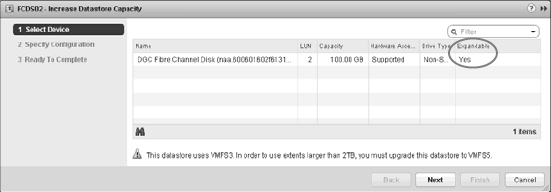
If you added an extent to the datastore, the datastore properties pane in Datastores And Datastore Clusters view will reflect the fact that the datastore now has at least two extents. This is also shown in the Datastore Properties dialog box, as you can see in Figure 6.38.
FIGURE 6.38 This 20 GB data-store actually comprises two 10 GB extents.
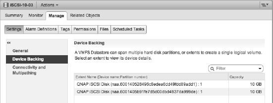
Regardless of the procedure used to expand the datastore, it is nondisruptive—there is no need to evacuate VMs or incur downtime.
Another nondisruptive task is upgrading a datastore from VMFS-3 to VMFS-5, a procedure that we describe in the following section.
UPGRADING A DATASTORE FROM VMFS-3 TO VMFS-5
As we described in “Examining the vSphere Virtual Machine File System,” vSphere 5.0 introduced a new version of VMFS called VMFS-5. VMFS-5 offers a number of new features. To take advantage of these new features, you'll need to upgrade your VMFS datastores from VMFS-3 to VMFS-5. Keep in mind that upgrading your datastores to VMFS-5 is required only if you need to take advantage of the features available in VMFS-5.
To help vSphere administrators keep clear about which datastores are VMFS-3 and which datastores are VMFS-5, VMware added that information in multiple places through the vSphere Web Client. Figure 6.39 shows the Configuration tab for an ESXi host; note that the datastore listing in the Storage section includes a column for VMFS version.
FIGURE 6.39 The columns in the Datastores list can be rearranged and reordered, and they include a column for VMFS version.
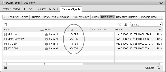
Figure 6.40 shows the details pane for a datastore, found on the Configuration tab for a data-store in Datastores And Datastore Clusters view. Again, note that the VMFS version is included in the information provided about that datastore. This view, by the way, is also a great view to see information about storage capabilities (used by policy-driven storage), the path policy in use, and whether or not Storage I/O Control is enabled for this datastore. The datastore in Figure 6.40 does have a user-defined storage capability assigned and has Storage I/O Control enabled.
FIGURE 6.40 Among the other details listed for a datastore, the VMFS version is also included.
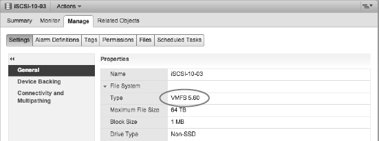
Perform the following steps to upgrade a datastore from VMFS-3 to VMFS-5:
- Log into the vSphere Web Client, if it isn't already running.
- Navigate to the Storage view and select a datastore from the Navigator list.
- Select the Manage tab and the Settings subsection.
- Under the General area, click the Upgrade To VMFS-5 button.
- If you are clear to proceed—meaning that all hosts attached are running at least ESXi 5.0 and support VMFS-5—a dialog box will appear to that effect. Click OK to start the upgrade of the datastore.
- The VMFS-5 upgrade will start. A task will appear in the Tasks pane for the upgrade; when the upgrade is complete, the vSphere Web Client will trigger a VMFS rescan on the attached hosts so that they also recognize that the datastore has been upgraded to VMFS-5.
After a datastore has been upgraded to VMFS-5, you cannot downgrade it back to VMFS-3.
ONE POTENTIAL REASON NOT TO UPGRADE VMFS-3 DATASTORES
Although you can upgrade a VMFS-3 datastore to VMFS-5, the underlying block size of the datastore does not change. This means that you could run into situations where Storage vMotion operations between an upgraded VMFS-3 datastore and a newly created VMFS-5 datastore could be slower than expected. This is because vSphere won't take advantage of hardware offloads when the block sizes are different between the source and destination datastores. For this reason, you might prefer (and we would recommend) to migrate your VMs off the VMFS-3 datastore and re-create it as a native VMFS-5 datastore instead of upgrading it.
We'd like to make one final note about VMFS versions. You'll note in the screen shot in Figure 6.40 that the selected datastore is running VMFS 5.60. vSphere 5.5 uses VMFS version 3.60 and VMFS version 5.60. For datastores running previous versions of VMFS-3 (say, VMFS 3.46), there is no need or any way to upgrade to VMFS 3.60. VMware only provides an upgrade path for moving from VMFS-3 to VMFS-5.
Figure 6.40 shows a datastore that has a user-defined storage capability assigned. As you know already, this is part of the functionality of policy-driven storage. Let's take a look at how to assign a capability to a datastore.
ASSIGNING A STORAGE CAPABILITY TO A DATASTORE
As we explained in “Examining Policy-Driven Storage,” you can define your own set of storage capabilities. These user-defined storage capabilities will be used with system-provided storage capabilities (supplied by VASA) in determining the compliance or noncompliance of a VM with its assigned VM storage policy. We'll discuss the creation of VM storage policies and compliance later in this chapter in the section “Assigning VM Storage Policies.” In this section, we'll just show you how to assign a user-defined storage capability to a datastore.
Perform these steps to assign a user-defined storage capability to a datastore:
- Launch the vSphere Web Client if it's not already running, and connect to a vCenter Server instance.
Policy-driven storage requires vCenter Server.
- Navigate to VM Storage Policies from the home screen.
- Click the icon labeled Enable VM Storage Polices.
This brings up the Enable VM Storage Polices dialog box, captured in Figure 6.41.
FIGURE 6.41 From this dialog box, you can enable or disable storage policies on a per-cluster level.
- Select the cluster for which you want to use storage polices and click the Enable button.
- When storage policies are enabled, click the Close button on the dialog box.
After you have created a storage capability (as explained in the section Examining Policy-Driven Storage) and the cluster is enabled for storage polices, you simply assign the tag you associated with the storage policy to the datastore itself. This provides the link between the storage policy and the datastore.
- From the vSphere Web Client Storage view, right-click a datastore and select Assign Tag.
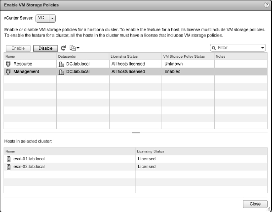
vCenter Server will assign the selected capability to the datastore, and it will show up in the datastore details view you saw previously in Figure 6.40.
Prior to vSphere 5.5, storage capabilities were directly assigned to a datastore. As you can see from the steps just outlined, the process is slightly different and uses tags to create a link between a datastore and a storage policy.
There are other datastore properties that you might also need to edit or change, such as renaming a datastore. We'll describe that process in the next section.
RENAMING A VMFS DATASTORE
You can rename a VMFS datastore in two ways:
- Right-click a datastore object and select Rename.
- When a datastore is selected in the Navigator, the Actions drop-down menu next to its name in the content area also has the rename command.
Both methods will produce the same result; the datastore will be renamed. You can use whichever method best suits you.
Modifying the multipathing policy for a VMFS datastore is another important function with which any vSphere administrator should be familiar.
MODIFYING THE MULTIPATHING POLICY FOR A VMFS DATASTORE
In the section “Reviewing Multipathing,” we described vSphere's Pluggable Storage Architecture (PSA) and how it manages multipathing for block-based storage devices. VMFS datastores are built on block-based storage devices, and so viewing or changing the multipathing configuration for a VMFS datastore is an integral part of working with VMFS datastores.
Changing the multipathing policy for a VMFS datastore is done using the Manage Paths button under the Datastore Manage tab in the Settings subsection. We've highlighted the Edit Multipathing button in Figure 6.42.
FIGURE 6.42 You'll use the Edit Multipathing button in the Datastore Manage ![]() Settings area to modify the multipathing policy.
Settings area to modify the multipathing policy.
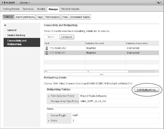
When you select Edit Multipathing, the Edit Multipathing Policies dialog box comes up (Figure 6.43). From this screen shot and from the information we've provided in this chapter, you should be able to deduce a few key facts:
FIGURE 6.43 This datastore resides on an active-active array; specifically, an EMC VNX. You can tell this by the currently assigned path selection policy and the storage array type information.
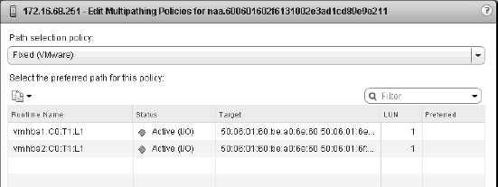
- This VMFS datastore is hosted on an active-active storage array; the currently assigned policy is Fixed (VMware), which is the default for an active-active array.
- This VMFS datastore resides on the first LUN hosted by an EMC VNX array. This is noted by the LUN column and also the L1 in the runtime name.
To change the multipathing policy, simply select a new policy from the Path Selection Policy drop-down list and click OK. One word of caution: Choosing the wrong path selection policy for your specific storage array can cause problems, so be sure to choose a path selection policy recommended by your storage vendor. In this particular case, the Round Robin policy is also supported by active-active arrays such as the EMC VNX hosting this LUN, so we'll change the path selection to Round Robin (VMware).
Changes to the path selection are immediate and do not require a reboot.
We're nearing the end of the discussion of VMFS datastores, but we do need to cover two more topics. First, we'll discuss managing copies of VMFS datastores, and then we'll wrap up this discussion with a quick review of removing VMFS datastores.
MANAGING VMFS DATASTORE COPIES
Every VMFS datastore has a universally unique identifier (UUID) embedded in the file system. When you clone or replicate a VMFS datastore, the copy of the datastore is a byte-for-byte copy, right down to the UUID. If you attempt to mount the LUN that has the copy of the VMFS data-store, vSphere will see this as a duplicate copy and will require that you do one of two things:
- Unmount the original and mount the copy with the same UUID.
- Keep the original mounted and write a new signature to the copy.
Other storage operations might also cause this behavior. If you change the LUN ID after creating a VMFS datastore, vSphere will recognize that the UUID is now associated with a new device (vSphere uses the NAA ID to track the devices) and will follow this behavior.
In either case, vSphere provides a GUI in the Add Storage Wizard that allows you to clearly choose which option you'd like to use in these situations:
- Choose Keep Existing Signature if you want to mount the datastore copy without writing a new signature. vSphere won't allow UUID collisions, so you can mount without resignaturing only if the original datastore has been unmounted or no longer exists (this is the case if you change the LUN ID, for example). If you mount a datastore copy without resignaturing and then later want to mount the original, you'll need to unmount the copy first.
- Choose Assign A New Signature if you want to write a new signature onto the VMFS datastore. This will allow you to have both the copy and the original mount as separate and distinct datastores. Keep in mind that this process is irreversible—you can't undo the resignaturing operation. If the resignatured datastore contains any VMs, you will likely need to reregister those VMs in vCenter Server because the paths to the VM's configuration files will have changed. The section “Adding or Registering Existing VMs” in Chapter 9 describes how to reregister a VM.
Let's take a look at removing a VMFS datastore.
REMOVING A VMFS DATASTORE
Removing a VMFS datastore is, fortunately, as straightforward as it seems. To remove a VMFS datastore, simply right-click the datastore object and select All vCenter Actions ![]() Delete Datastore. The vSphere Web Client will prompt for confirmation—reminding you that you will lose all the files associated with all VMs on this datastore—before actually deleting the datastore.
Delete Datastore. The vSphere Web Client will prompt for confirmation—reminding you that you will lose all the files associated with all VMs on this datastore—before actually deleting the datastore.
As with many of the other datastore-related tasks we've shown you, the vSphere Web Client will trigger a VMFS rescan for other ESXi hosts so that all hosts are aware that the VMFS data-store has been deleted.
Like resignaturing a datastore, deleting a datastore is irreversible. Once you delete a data-store, you can't recover the datastore or any of the files that were stored in it. Be sure to double-check that you're deleting the right datastore before you proceed!
Let's now shift from working with VMFS datastores to working with another form of block-based storage, albeit one that is far less frequently used: raw device mappings, or RDMs.
Working with Raw Device Mappings
Although the concept of shared pool mechanisms (like VMFS or NFS datastores) for VMs works well for many use cases, there are certain use cases where a storage device must be presented directly to the guest operating system (guest OS) inside a VM.
vSphere provides this functionality via a raw device mapping (RDM). RDMs are presented to your ESXi hosts and then via vCenter Server directly to a VM. Subsequent data I/O bypasses the VMFS and volume manager completely, though management is handled via a mapping file that is stored on a VMFS volume.
IN-GUEST ISCSI AS AN ALTERNATIVE TO RDMS
In addition to using RDMs to present storage devices directly to the guest OS inside a VM, you can use in-guest iSCSI software initiators. We'll provide more information on that scenario in the section “Using In-Guest iSCSI Initiators” later in this chapter.
RDMs should be viewed as a tactical tool in the vSphere administrators' toolkit rather than as a common use case. A common misconception is that RDMs perform better than VMFS. In reality, the performance delta between the storage types is within the margin of error of tests. Although it is possible to oversubscribe a VMFS or NFS datastore (because they are shared resources) and not an RDM (because it is presented to specific VMs only), this is better handled through design and monitoring rather than through the extensive use of RDMs. In other words, if your concerns about oversubscription of a storage resource are driving the choice of an RDM over a shared datastore model, simply choose to not put multiple VMs in the pooled datastore.
You can configure RDMs in two different modes:
Physical Compatibility Mode (pRDM) In this mode, all I/O passes directly through to the underlying LUN device, and the mapping file is used solely for locking and vSphere management tasks. Generally, when a storage vendor says “RDM” without specifying further, it means physical compatibility mode RDM. You might also see this referred to as a pass-through disk.
Virtual Mode (vRDM) In this mode, there is still a mapping file, but it enables more (not all) features that are supported with normal VMDKs. Generally, when VMware says “RDM” without specifying further, it means a virtual mode RDM.
Contrary to common misconception, both modes support almost all vSphere advanced functions such as vSphere HA and vMotion, but there is one important difference: virtual mode RDMs can be included in a vSphere snapshot, while physical mode RDMs cannot. This inability to take a native vSphere snapshot of a pRDM also means that features that depend on snapshots don't work with pRDMs. In addition, a virtual mode RDM can go from virtual mode RDM to a virtual disk via Storage vMotion, but a physical mode RDM cannot.
PHYSICAL OR VIRTUAL? BE SURE TO ASK!
When a feature specifies RDM as an option, make sure to check the type: physical compatibility mode or virtual mode.
The most common use case for RDMs are VMs configured as Microsoft Windows clusters. In Windows Server 2008, this is called Windows Failover Clusters (WFC), and in Windows Server 2003, this is called Microsoft Cluster Services (MSCS). In Chapter 7, the section “Introducing Windows Server Failover Clustering” provides full details on how to use RDMs with Windows Server–based clusters.
Another important use case of pRDMs is that they can be presented from a VM to a physical host interchangeably. This gives pRDMs a flexibility that isn't found with virtual mode RDMs or virtual disks. This flexibility is especially useful in cases where an independent software vendor (ISV) hasn't yet embraced virtualization and indicates that virtual configurations are not supported. In this instance, the RDMs can easily be moved to a physical host to reproduce the issue on a physical machine. For example, this is useful in Oracle on vSphere use cases.
In a small set of use cases, storage vendor features and functions depend on the guest directly accessing the LUN and therefore need pRDMs. For example, certain arrays, such as EMC Symmetrix, use in-band communication for management to isolate management from the IP network. This means the management traffic is communicated via the block protocol (most commonly Fibre Channel). In these cases, EMC gatekeeper LUNs are used for host-array communication and, if they are used in a VM (commonly where EMC Solutions Enabler is used), require pRDMs.
Finally, another example of storage features that are associated with RDMs are those related to storage array features such as application-integrated snapshot tools. These are applications that integrate with Microsoft Exchange, SQL Server, SharePoint, Oracle, and other applications to handle recovery modes and actions. Examples include EMC's Replication Manager, NetApp's SnapManager family, and Dell/EqualLogic's Auto Volume Replicator tools. Previous generations of these tools required the use of RDMs, but most of the vendors now can manage these without the use of RDMs and integrate with vCenter Server APIs. Check with your array vendor for the latest details.
In Chapter 7, we show you how to create an RDM, and we briefly discuss RDMs in Chapter 9.
We're now ready to shift away from block-based storage in a vSphere environment and move into a discussion of working with NAS/NFS datastores.
Working with NFS Datastores
NFS datastores are used in much the same way as VMFS datastores: as shared pools of storage for VMs. Although VMFS and NFS are both shared pools of storage for VMs, they are different in other ways. The two most important differences between VMFS and NFS datastores are as follows:
- With NFS datastores the file system itself is not managed or controlled by the ESXi host; rather, ESXi is using the NFS protocol via an NFS client to access a remote file system managed by the NFS server.
- With NFS datastores all the vSphere elements of high availability and performance scaling design are not part of the storage stack but are part of the networking stack of the ESXi host.
These differences create some unique challenges in properly architecting an NFS-based solution. This is not to say that NFS is in any way inferior to block-based storage protocols; rather, the challenges that NFS presents are simply different challenges that many storage-savvy vSphere administrators have probably not encountered before. Networking-savvy vSphere administrators will be quite familiar with some of these behaviors, which center on the use of link aggregation and its behavior with TCP sessions.
Before going into detail on how to create or remove an NFS datastore, we'd like to first address some of the networking-related considerations.
CRAFTING A HIGHLY AVAILABLE NFS DESIGN
High-availability design for NFS datastores is substantially different from that of block storage devices. Block storage devices use MPIO, which is an end-to-end path model. For Ethernet networking and NFS, the domain of link selection is from one Ethernet MAC to another Ethernet MAC, or one link hop. This is configured from the host to switch, from switch to host, and from NFS server to switch and switch to NFS server; Figure 6.44 shows the comparison. In the figure, “link aggregation” refers to NIC teaming where multiple connections are bonded together for greater aggregate throughput (with some caveats, as we'll explain in a moment).
FIGURE 6.44 NFS uses the networking stack, not the storage stack, for high availability and load balancing.
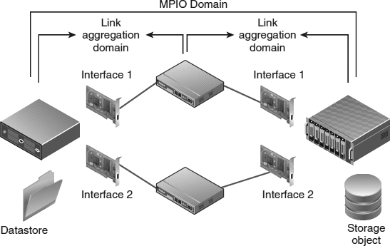
The mechanisms used to select one link or another are fundamentally the following:
- A NIC teaming/link aggregation choice, which is set up per TCP connection and is either static (set up once and permanent for the duration of the TCP session) or dynamic (can be renegotiated while maintaining the TCP connection, but still always on only one link or the other).
- A TCP/IP routing choice, where an IP address (and the associated link) is selected based on layer 3 routing—note that this doesn't imply that traffic crosses subnets via a gateway, only that the ESXi host selects the NIC or a given datastore based on the IP subnet.
Figure 6.45 shows the basic decision tree.
FIGURE 6.45 The choices to configure highly available NFS datastores depend on your network infrastructure and configuration.
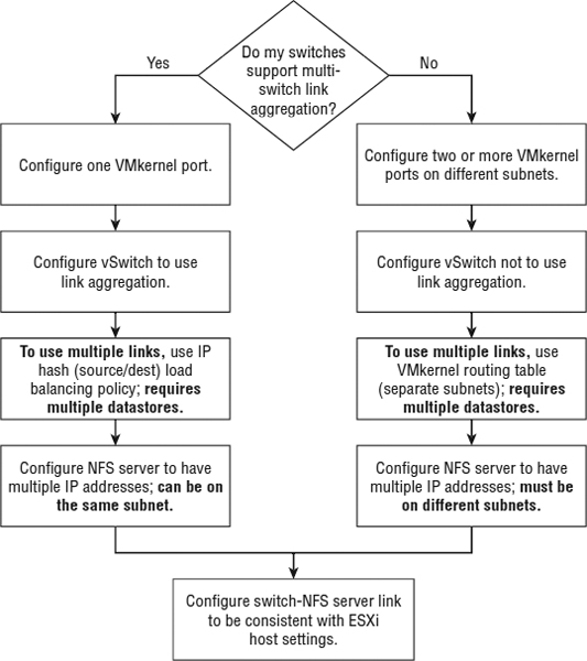
The path on the left has a topology that looks like Figure 6.46. Note that the little arrows mean that link aggregation/static teaming is configured from the ESXi host to the switch and on the switch to the ESXi host; in addition, note that there is the same setup on both sides for the relationship between the switch and the NFS server.
FIGURE 6.46 If you have a network switch that supports multi-switch link aggregation, you can easily create a network team that spans switches.
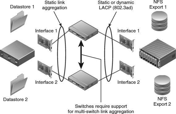
The path on the right has a topology that looks like Figure 6.47. You can use link aggregation/teaming on the links in addition to the routing mechanism, but this has limited value—remember that it won't help with a single datastore. Routing is the selection mechanism for the outbound NIC for a datastore, and each NFS datastore should be reachable via an alias on both subnets.
FIGURE 6.47 If you have a basic network switch without multi-switch link aggregation or don't have the experience or control of your network infrastructure, you can use VMkernel routing by placing multiple VMkernel network interfaces on separate vSwitches and different subnets.
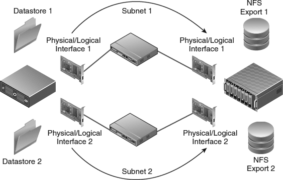
The key to understanding why NIC teaming and link aggregation techniques cannot be used to scale up the bandwidth of a single NFS datastore is how TCP is used in the NFS case. Remember that the MPIO-based multipathing options used for block storage and iSCSI in particular are not options here because NFS datastores use the networking stack, not the storage stack. The VMware NFS client uses two TCP sessions per datastore (as shown in Figure 6.48): one for control traffic and one for data flow. The TCP connection for the data flow is the vast majority of the bandwidth. With all NIC teaming/link aggregation technologies, Ethernet link choice is based on TCP connections. This happens either as a one-time operation when the connection is established with NIC teaming or dynamically, with 802.3ad. Regardless, there's always only one active link per TCP connection and therefore only one active link for all the data flow for a single NFS datastore.
FIGURE 6.48 Every NFS datastore has two TCP connections to the NFS server but only one for data.
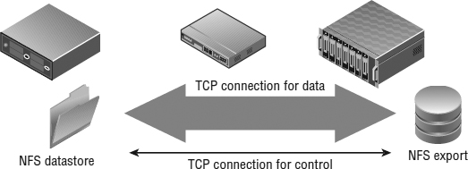
This highlights that, as with VMFS, the “one big datastore” model is not a good design principle. In the case of VMFS, it's not a good model because of the extremely large number of VMs and the implications on LUN queues (and to a far lesser extent, SCSI locking impact). In the case of NFS, it is not a good model because the bulk of the bandwidth would be on a single TCP session and therefore would use a single Ethernet link (regardless of network interface teaming, link aggregation, or routing). This has implications for supporting high-bandwidth workloads on NFS, as we'll explore later in this section.
Another consideration of highly available design with NFS datastores is that NAS device failover is generally longer than for a native block device. Block storage devices generally can fail over after a storage processor failure in seconds (or milliseconds). NAS devices, on the other hand, tend to fail over in tens of seconds and can take longer depending on the NAS device and the configuration specifics. There are NFS servers that fail over faster, but these tend to be relatively rare in vSphere use cases. This long failover period should not be considered intrinsically negative but rather a configuration question that determines the fit for NFS datastores, based on the VM service-level agreement (SLA) expectation.
The key questions are these:
- How much time elapses before ESXi does something about a datastore being unreachable?
- How much time elapses before the guest OS does something about its virtual disk not responding?
FAILOVER IS NOT UNIQUE TO NFS
The concept of failover exists with Fibre Channel and iSCSI, though, as noted in the text, it is generally in shorter time intervals. This time period depends on specifics of the HBA configuration, but typically it is less than 30 seconds for Fibre Channel/FCoE and less than 60 seconds for iSCSI. Depending on your multipathing configuration within vSphere, path failure detection and switching to a different path might be much faster (nearly instantaneous).
The answer to both questions is a single word: time-outs. Time-outs exist at the vSphere layer to determine how much time should pass before a datastore is marked as unreachable, and time-outs exist within the guest OS to control the behavior of the guest OS. Let's look at each of these.
At the time of this writing, both EMC and NetApp recommend the same ESXi failover settings. Because these recommendations change, please be sure to refer to the latest recommendations from your storage vendor to be sure you have the right settings for your environment. Based on your storage vendor's recommendations, you can change the time-out value for NFS datastores by changing the values in the Advanced Settings dialog box, shown in Figure 6.49.
FIGURE 6.49 When configuring NFS datastores, it's important to extend the ESXi host time-outs to match the vendor best practices. This host is not configured with the recommended settings.

The current settings (at the time of this writing) that both EMC and NetApp recommend are as follows:
- NFS.HeartbeatDelta: 12
- NFS.HeartbeatTimeout: 5
- NFS.HeartbeatMaxFailures: 10
You should configure these settings across all ESXi hosts that will be connected to NFS datastores.
Here's how these settings work:
- Every NFS.HeartbeatDelta (or 12 seconds), the ESXi host checks to see that the NFS data-store is reachable.
- Those heartbeats expire after NFS.HeartbeatTimeout (or 5 seconds), after which another heartbeat is sent.
- If NFS.HeartbeatMaxFailures (or 10) heartbeats fail in a row, the datastore is marked as unavailable, and the VMs crash.
This means that the NFS datastore can be unavailable for a maximum of 125 seconds before being marked unavailable, which covers the large majority of failover events (including those for both NetApp and EMC NAS devices serving NFS to a vSphere environment).
What does a guest OS see during this period? It sees a nonresponsive SCSI disk on the vSCSI adapter (similar to the failover behavior of a Fibre Channel or iSCSI device, though the interval is generally shorter). The disk time-out is how long the guest OS will wait while the disk is nonresponsive before throwing an I/O error. This error is a delayed write error, and for a boot volume it will result in the guest OS crashing. Windows Server, for example, has a disk timeout default of 60 seconds. A recommendation is to increase the guest OS disk time-out value to match the NFS datastore time-out value. Otherwise, the VMs can timeout their boot storage (which will cause a crash) while ESXi is still waiting for the NFS datastore within the longer time-out value. Without extending the guest time-out, if vSphere HA is configured for VM monitoring, the VMs will reboot (when the NFS datastore returns), but obviously extending the time-out is preferable to avoid this extra step and the additional delay and extra I/O workload it generates.
Perform the following steps to set operating system time-out for Windows Server to match the 125-second maximum set for the datastore. You'll need to be logged into the Windows Server system as a user who has administrative credentials.
- Back up your Windows Registry.
- Select Start Run, type regedit.exe, and click OK.
- In the left panel hierarchy view, double-click HKEY_LOCAL_MACHINE, then System, then CurrentControlSet, then Services, and then Disk.
- Select the TimeOutValue value, and set the data value to 125 (decimal).
There are two sub-cases of NFS that we want to examine briefly before we start showing you how to create and manage NFS datastores: large bandwidth workloads and large throughput workloads. Each of these cases deserves a bit of extra attention when planning your highly available design for NFS.
Supporting Large Bandwidth (MBps) Workloads on NFS
Bandwidth for large I/O sizes is generally gated by the transport link (in this case the TCP session used by the NFS datastore being 1 Gbps or 10 Gbps) and overall network design. At larger scales, you should apply the same care and design as you would for iSCSI or Fibre Channel networks. In this case, it means carefully planning the physical network/VLAN, implementing end-to-end jumbo frames, and leveraging enterprise-class Ethernet switches with sufficient buffers to handle significant workload. At 10 GbE speeds, features such as TCP Segment Offload (TSO) and other offload mechanisms, as well as the processing power and I/O architecture of the NFS server, become important for NFS datastore and ESXi performance.
So, what is a reasonable performance expectation for bandwidth on an NFS datastore? From a bandwidth standpoint, where 1 Gbps Ethernet is used (which has 2 Gbps of bandwidth bidirectionally), the reasonable bandwidth limits are 80 MBps (unidirectional 100 percent read or 100 percent write) to 160 MBps (bidirectional mixed read/write workloads) for a single NFS data-store. That limits scale accordingly with 10 Gigabit Ethernet. Because of how TCP connections are handled by the ESXi NFS client, and because of how networking handles link selection in link aggregation or layer 3 routing decisions, almost all the bandwidth for a single NFS datastore will always use only one link. If you therefore need more bandwidth from an NFS datastore than a single Gigabit Ethernet link can provide, you have no other choice than to migrate to 10 Gigabit Ethernet, because link aggregation won't help (as we explained earlier).
Supporting Large Throughput (IOPS) Workloads on NFS
High-throughput (IOPS) workloads are usually gated by the backend configuration (as true of NAS devices as it is with block devices) and not the protocol or transport since they are also generally low bandwidth (MBps). By backend, we mean the array target. If the workload is cached, then it's determined by the cache response, which is almost always astronomical. However, in the real world, most often the performance is not determined by cache response; the performance is determined by the spindle configuration that supports the storage object. In the case of NFS datastores, the storage object is the file system, so the considerations that apply at the ESXi host for VMFS (disk configuration and interface queues) apply within the NFS server. Because the internal architecture of an NFS server varies so greatly from vendor to vendor, it's almost impossible to provide recommendations, but here are a few examples. On a NetApp FAS array, the IOPS achieved is primarily determined by the FlexVol/aggregate/RAID group configuration. On an EMC VNX array, it is likewise primarily determined by the Automated Volume Manager/dVol/RAID group configuration. Although there are other considerations (at a certain point, the scale of the interfaces on the array and the host's ability to generate I/Os become limited, but up to the limits that users commonly encounter), performance is far more often constrained by the backend disk configuration that supports the file system. Make sure your file system has sufficient backend spindles in the container to deliver performance for all the VMs that will be contained in the file system exported via NFS.
With these NFS storage design considerations in mind, let's move forward with creating and mounting an NFS datastore.
THERE'S ALWAYS AN EXCEPTION TO THE RULE
Thus far, we've been talking about how NFS always uses only a single link, and how you always need to use multiple VMkernel ports and multiple NFS exports in order to utilize multiple links.
Normally, vSphere requires that you mount an NFS datastore using the same IP address or hostname and path on all hosts. vSphere 5.0 added the ability to use a DNS hostname that resolves to multiple IP addresses. However, each vSphere host will resolve the DNS name only once. This means that it will resolve to only a single IP address and will continue to use only a single link. In this case, there is no exception to the rule. However, this configuration can provide some rudimentary load balancing for multiple hosts accessing a datastore via NFS over multiple links.
CREATING AND MOUNTING AN NFS DATASTORE
In this procedure, we will show you how to create and mount an NFS datastore in vSphere. The term create here is a bit of a misnomer; the file system is actually created on the NFS server and just exported. That process we can't really show you, because the procedures vary so greatly from vendor to vendor. What works for one vendor to create an NFS datastore is likely to be different for another vendor.
Before you start, ensure that you've completed the following steps:
- You created at least one VMkernel port for NFS traffic. If you intend to use multiple VMkernel ports for NFS traffic, ensure that you configure your vSwitches and physical switches appropriately, as described in “Crafting a Highly Available NFS Design.”
- You configured your ESXi host for NFS storage according to the vendor's best practices, including time-out values and any other settings. At the time of this writing, many storage vendors recommend an important series of advanced ESXi parameter settings to maximize performance (including increasing memory assigned to the networking stack and changing other characteristics). Be sure to refer to your storage vendor's recommendations for using its product with vSphere.
- You created a file system on your NAS device and exported it via NFS. A key part of this configuration is the specifics of the NFS export itself; the ESXi NFS client must have full root access to the NFS export. If the NFS export was exported with root squash, the file system will not be able to mount on the ESXi host. (Root users are downgraded to unprivileged file system access. On a traditional Linux system, when root squash is configured on the export, the remote systems are mapped to the “nobody” account.) You have one of two options for NFS exports that are going to be used with ESXi hosts:
- Use the no_root_squash option, and give the ESXi hosts explicit read/write access.
- Add the ESXi host's IP addresses as root-privileged hosts on the NFS server.
For more information on setting up the VMkernel networking for NFS traffic, refer to Chapter 5; for more information on setting up your NFS export, refer to your storage vendor's documentation.
After you complete these steps, you're ready to mount an NFS datastore.
Perform the following steps to mount an NFS datastore on an ESXi host:
- Make a note of the IP address on which the NFS export is hosted as well as the name (and full path) of the NFS export; you'll need this information later in this process.
- Launch the vSphere Web Client and connect to an ESXi host or to a vCenter Server instance.
- In the vSphere Web Client, navigate to the Storage view.
- Right-click the datacenter object and select All vCenter Actions New Datastore. This launches the New Datastore Wizard.
- At the Storage Type screen, select Network File System. Click Next.
- At the Name And Configuration screen, you'll need to supply three pieces of information:
- First, you'll need to supply a datastore name. As with VMFS datastores, we recommend a naming scheme that identifies the NFS server and other pertinent information for easier troubleshooting.
- You'll need to supply the IP address on which the NFS export is hosted. If you don't know this information, you'll need to go back to your storage array and determine what IP address it is using to host the NFS export. In general, identifying the NFS server by IP addresses is recommended, but it is not recommended to use a hostname because it places an unnecessary dependency on DNS and because generally it is being specified on a relatively small number of hosts. There are, of course, some cases where a hostname may be applicable—for example, where NAS virtualization techniques are used to provide transparent file mobility between NFS servers—but this is relatively rare. Also, refer to the sidebar titled “There's Always an Exception to the Rule”; that sidebar describes another configuration in which you might want to use a hostname that resolves to multiple IP addresses.
- You'll need to supply the folder or path to the NFS export. Again, this is determined by the NFS server and the settings on the NFS export.
Figure 6.50 shows an example of the Name And Configuration screen of the New Datastore wizard, where we've supplied the necessary information.
FIGURE 6.50 Mounting an NFS datastore requires that you know the IP address and the export name from the NFS server.
- If the NFS datastore should be read-only, then select Mount NFS As Read Only.
You might need to mount a read-only NFS datastore if the datastore contains only ISO images, for example.
When you click Next to continue, your server IP and folder path will be validated.
- On the following screen you can select one or multiple hosts to connect to this datastore.
- Review the information at the summary screen. If everything is correct, click Finish to continue; otherwise, go back and make the necessary changes.

When you click Finish, the vSphere Web Client will mount the NFS datastore on the selected ESXi host and the new NFS datastore will appear in the list of datastores, as you can see in Figure 6.51.
FIGURE 6.51 NFS datastores are listed in among VMFS datastores, but the information provided for each is different.
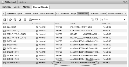
TROUBLESHOOTING NFS CONNECTIVITY
If you're having problems getting an NFS datastore to mount, the following list can help you trouble-shoot the problem:
- Can you ping the IP address of the NFS export from the ESXi host? (Use the Direct Console User Interface [DCUI] to test connectivity from the ESXi host, or enable the ESXi shell and use the vmkping command.)
- Is the physical cabling correct? Are the link lights showing a connected state on the physical interfaces on the ESXi host, the Ethernet switches, and the NFS server?
- Are your VLANs configured correctly? If you've configured VLANs, have you properly configured the same VLAN on the host, the switch, and the interface(s) that will be used on your NFS server?
- Is your IP routing correct and functional? Have you properly configured the IP addresses of the VMkernel port and the interface(s) that will be used on the NFS server? Are they on the same subnet? If not, they should be. Although you can route NFS traffic, it's not a good idea because routing adds significant latency and isn't involved in a bet-the-business storage Ethernet network. In addition, it's generally not recommended in vSphere environments.
- Is the NFS traffic being allowed through any firewalls? If the ping succeeds but you can't mount the NFS export, check to see if NFS is being blocked by a firewall somewhere in the path. Again, the general recommendation is to avoid firewalls in the midst of the data path wherever possible to avoid introducing additional latency.
- Are jumbo frames configured correctly? If you're using jumbo frames, have you configured jumbo frames on the VMkernel port, the vSwitch or distributed vSwitch, all physical switches along the data path, and the NFS server?
- Are you allowing the ESXi host root access to the NFS export?
Unlike VMFS datastores in vSphere, you need to add the NFS datastore on each host in the vSphere environment. Also, it's important to use consistent NFS properties (for example, a consistent IP/domain name) as well as common datastore names; this is not enforced. VMware provides a helpful reminder on the Name And Configuration screen, which you can see in Figure 6.50. In the vSphere 5.5 Web Client you now have the ability to add additional hosts to an existing NFS datastore without needing the NFS server IP and folder. Simply right-click an NFS datastore and select All vCenter Actions ![]() Mount Datastore To Additional Host.
Mount Datastore To Additional Host.
After the NFS datastore is mounted, you can use it as you would any other datastore—you can select it as a Storage vMotion source or destination, you can create virtual disks on it, or you can map ISO images stored on an NFS datastore into a VM as a virtual CD/DVD drive.
As you can see, using NFS requires a simple series of steps, several fewer than using VMFS. And yet, with the same level of care, planning, and attention to detail, you can create robust NFS infrastructures that provide the same level of support as traditional block-based storage infrastructures.
So far we've examined both block-based storage and NFS-based storage at the hypervisor level. But what if you need a storage device presented directly to a VM, not a shared container, as is the case with VMFS and NFS datastores? The next sections discuss some common VM-level storage configuration options.
Working with VM-Level Storage Configuration
Let's move from ESXi- and vSphere-level storage configuration to the storage configuration details for individual VMs.
First, we'll review virtual disks and the types of virtual disks supported in vSphere. Next we'll review the virtual SCSI controllers. Then we'll move into a discussion of VM storage policies and how to assign them to a VM, and we'll wrap up this discussion with a brief exploration of using an in-guest iSCSI initiator to access storage resources.
INVESTIGATING VIRTUAL DISKS
Virtual disks (referred to as VMDKs because of the filename extension used by vSphere) are how VMs encapsulate their disk devices (if not using RDMs), and they warrant further discussion. Figure 6.52 shows the properties of a VM. Hard disk 1 is a 30 GB thick-provisioned virtual disk on a VMFS datastore. Hard disk 2, conversely, is an RDM.
FIGURE 6.52 This VM has both a virtual disk on a VMFS datastore and an RDM.
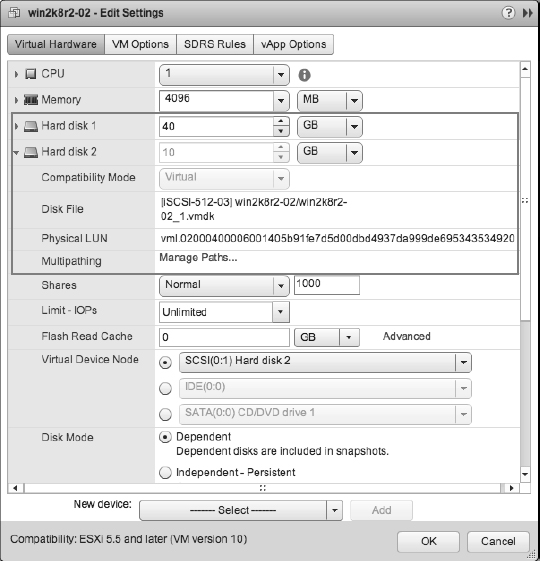
We discussed RDMs previously in the section “Working with Raw Device Mappings,” and we'll discuss RDMs in a bit more detail in Chapter 7 as well. As you know already, RDMs are used to present a storage device directly to a VM instead of encapsulating the disk into a file on a VMFS datastore.
Virtual disks come in three formats:
Thin-Provisioned Disk In this format, the size of the VDMK file on the datastore is only as much as is used (or was at some point used) within the VM itself. The top of Figure 6.53 illustrates this concept. For example, if you create a 500 GB virtual disk and place 100 GB of data in it, the VMDK file will be 100 GB in size. As I/O occurs in the guest, the VMkernel zeroes out the space needed right before the guest I/O is committed and grows the VMDK file similarly. Sometimes, this is referred to as a sparse file. Note that space deleted from the guest OS's file system won't necessarily be released from the VMDK; if you added 50 GB of data but then turned around and deleted 50 GB of data, the space wouldn't necessarily be released to the hypervisor so that the VMDK can shrink in size. (Some guest OSes support the necessary T10 SCSI commands to address this situation.)
FIGURE 6.53 A thin-provisioned virtual disk uses only as much as the guest OS in the VM uses. A flat disk doesn't pre-zero unused space, so an array with thin provisioning would show only 100 GB used. A thickly provisioned (eager zeroed) virtual disk consumes 500 GB immediately because it is pre-zeroed.
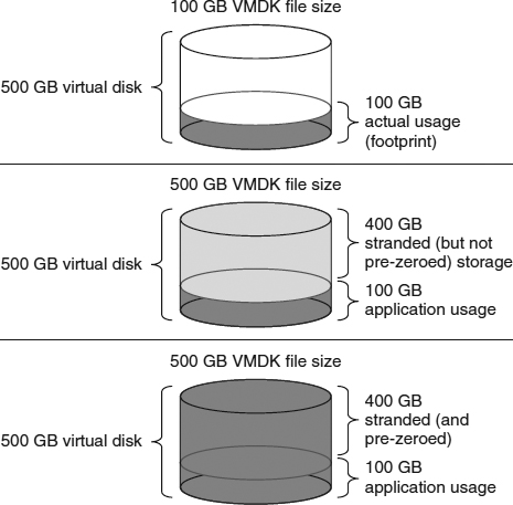
Thick Provisioned Lazy Zeroed In this format (sometimes referred to as a flat disk), the size of the VDMK file on the datastore is the size of the virtual disk that you create, but within the file, it is not pre-zeroed at the time of initial creation. For example, if you create a 500 GB virtual disk and place 100 GB of data in it, the VMDK will appear to be 500 GB at the datastore file system, but it contains only 100 GB of data on disk. This is shown in center of Figure 6.53. As I/O occurs in the guest, the VMkernel zeroes out the space needed right before the guest I/O is committed, but the VDMK file size does not grow (since it was already 500 GB).
Thick Provisioned Eager Zeroed Thick provisioned eager zeroed virtual disks, also referred to as eagerly zeroed disks or eagerzeroedthick disks, are truly thick. In this format, the size of the VDMK file on the datastore is the size of the virtual disk that you create, and within the file, it is pre-zeroed, as illustrated at the bottom of Figure 6.53. For example, if you create a 500 GB virtual disk and place 100 GB of data in it, the VMDK will appear to be 500 GB at the datastore file system, and it contains 100 GB of data and 400 GB of zeros on disk. As I/O occurs in the guest, the VMkernel does not need to zero the blocks prior to the I/O occurring. This results in slightly improved I/O latency and fewer backend storage I/O operations during initial I/O operations to new allocations in the guest OS, but it results in significantly more backend storage I/O operation up front during the creation of the VM. If the array supports VAAI, vSphere can offload the up-front task of zeroing all the blocks and reduce the initial I/O and time requirements.
This third type of virtual disk occupies more space than the first two, but it is required if you are going to use vSphere FT. (If they are thin-provisioned or flat virtual disks, conversion occurs automatically when the vSphere FT feature is enabled.)
As you'll see in Chapter 12 when we discuss Storage vMotion, you can convert between these virtual disk types using Storage vMotion.
ALIGNING VIRTUAL DISKS
Do you need to align the virtual disks? The answer is it depends on the guest operating system. Although not absolutely mandatory, it's recommended that you follow VMware's recommended best practices for aligning the volumes of guest OSes—and do so across all vendor platforms and all storage types. These are the same as the very mature standard techniques for aligning the partitions in standard physical configurations from most storage vendors.
Why do this? Aligning a partition aligns the I/O along the underlying RAID stripes of the array, which is particularly important in Windows environments (Windows Server from 2008 onward automatically aligns partitions). This alignment step minimizes the extra I/Os by aligning the I/Os with the array RAID stripe boundaries. Extra I/O work is generated when the I/Os cross the stripe boundary with all RAID schemes as opposed to a full stripe write. Aligning the partition provides a more efficient use of what is usually the most constrained storage array resource—IOPS. If you align a template and then deploy from a template, you maintain the correct alignment.
Why is it important to do this across vendors and across protocols? Changing the alignment of the guest OS partition is a difficult operation once data has been put in the partition—so it is best done up front when creating a VM or when creating a template.
Some of these types of virtual disks are supported in certain environments and others are not. VMFS datastores support all three types of virtual disks (thin, flat, and thick), but NFS datastores support only thin unless the NFS server supports the VAAIv2 NAS extensions and vSphere has been configured with the vendor-supplied plug-in. Figure 6.54 shows the screen for creating a new virtual disk for a VM (a procedure we'll describe in full detail in Chapter 9) on a VMFS datastore; the two thick provisioning options are not available if you are provisioning to an NFS datastore that does not have VAAIv2 support.
FIGURE 6.54 VMFS datastores support all three virtual disk types.
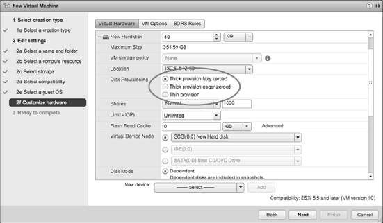
Is there a way to tell which type of virtual disk a VM is using? Certainly. In all three cases, the free space indication within the guest OS is always going to indicate the maximum size of the virtual disk, so you won't be able to use that. Fortunately, VMware provides several other ways to determine the disk type:
- In the Datastore Storage Reports subsection, vSphere includes columns for virtual disk space, uncommitted space, provisioned space, and space used. As you can see in Figure 6.55, the columns break out these statistics on a per-VM basis. This allows you to clearly see things like the maximum size of a thin-provisioned VM as well as the current space usage. By right-clicking on the columns, you can select other columns that are not shown in this screen shot, such as these:
- Cluster
- Resource Pool
- Multipathing Status
- % Space Used
- % Snapshot Space
- % Virtual Disk Space
- Swap Space
- % Swap Space
- Other VM Space
- % Other VM Space
- % Shared Space
FIGURE 6.55 The Space Used and Provisioned Space columns tell you the current and maximum space allocations for a thin-provisioned disk.
- On the Summary tab of a VM, the vSphere Web Client provides statistics on currently provisioned space, and used space. Figure 6.56 shows the statistics for a deployed instance of the vCenter Server virtual appliance.
FIGURE 6.56 The Summary tab of a VM will report the total provisioned space as well as the used space.
- Finally, the Edit Settings dialog box will also display the virtual disk type for a selected virtual disk in a VM. Using the same deployed instance of the vCenter virtual appliance as an example, Figure 6.57 shows the information supplied in this dialog box. You can't determine current space usage, but you can at least determine what type of disk is configured.
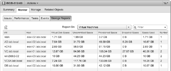
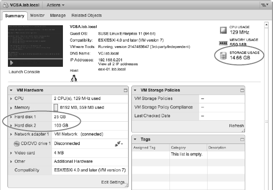
FIGURE 6.57 The Edit Settings dialog box tells you what kind of disk is configured, but doesn't provide current space usage statistics.
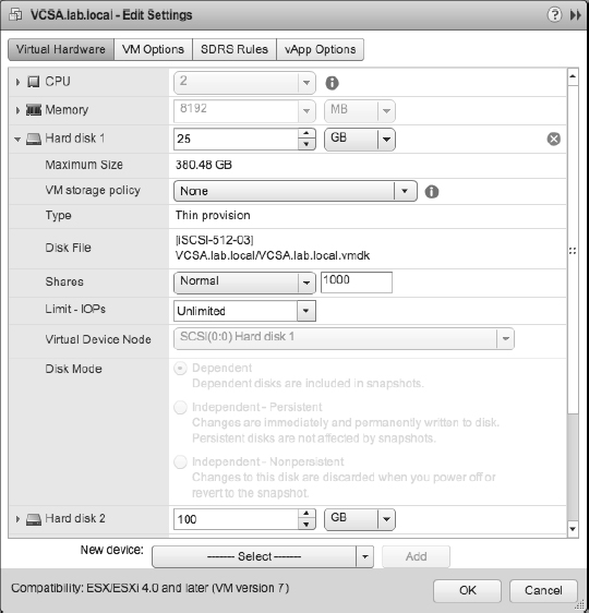
Closely related to virtual disks are the virtual SCSI adapters that are present within every VM.
EXPLORING VIRTUAL STORAGE ADAPTERS
You configure virtual storage adapters in your VMs, and you will attach these adapters to virtual disks and RDMs, just as a physical server needs an adapter to connect physical hard disks to. In the guest OS, each virtual storage adapter has its own HBA queue, so for intense storage workloads, there are advantages to configuring multiple virtual SCSI adapters within a single guest.
There are a number of different virtual storage adapters in ESXi, as shown in Figure 6.58.
FIGURE 6.58 There are various virtual SCSI adapters that a VM can use. You can configure up to four virtual SCSI adapters for each VM.
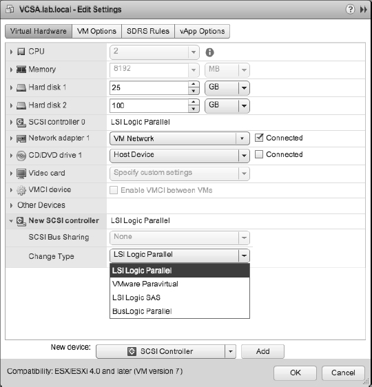
Table 6.3 summarizes the information about the five types of virtual storage adapters avail-able for you to use.
TABLE 6.3: Virtual SCSi and SATA storage adapters in vSphere 5.5
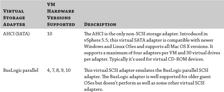
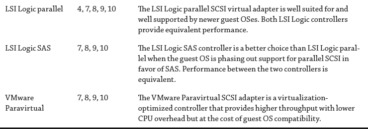
As you can see from Table 6.3, two of these adapters—the LSI Logic SAS and VMware Paravirtual—are available only for VM hardware version 7 or higher. The LSI Logic SAS controller is the default SCSI adapter suggested for VMs running Windows Server 2008 and 2008 R2, while the LSI Logic parallel SCSI controller is the default for Windows Server 2003. Many of the various Linux flavors default to the BusLogic parallel SCSI adapters.
The BusLogic and LSI Logic controllers are pretty straightforward; they emulate a known SCSI controller. The AHCI adapter is a SATA-based controller to replace the older IDE adapter. Typically this would only be used to support guest virtual CD-ROM drives. The VMware Paravirtual SCSI adapter, though, is a different kind of controller.
In short, paravirtualized devices (and their corresponding drivers) are specifically optimized to communicate more directly with the underlying VM Monitor (VMM); they deliver higher throughput and lower latency, and they usually significantly lower the CPU impact of the I/O operations. This is the case with the VMware Paravirtual SCSI adapter in vSphere. We'll discuss paravirtualized drivers in greater detail in Chapter 9.
Compared to other virtual SCSI adapters, the paravirtualized SCSI adapter shows improvements in performance for virtual disks as well as improvements in the number of IOPS delivered at any given CPU utilization. The paravirtualized SCSI adapter also shows improvements (decreases) in storage latency as observed from the guest OS.
If the paravirtualized SCSI adapter works so well, why not use it for everything? Well, for one, this is an adapter type that exists only in vSphere environments, so you won't find the drivers for the paravirtualized SCSI adapter on the install disk for most guest OSes. In general, we recommend using the virtual SCSI adapter suggested by vSphere for the boot disk and the para-virtualized SCSI adapter for any other virtual disks, especially other virtual disks with active workloads.
As you can see, there are lots of options for configuring VM-level storage. When you factor in different datastores and different protocol options, how can you ensure that VMs are placed on the right storage? This is where VM storage policies come into play.
ASSIGNING VM STORAGE POLICIES
VM storage policies are a key component of policy-driven storage. By leveraging system-provided storage capabilities supplied by a VASA provider (which is provided by the storage vendor), as well as user-defined storage capabilities, you can build VM storage policies that help shape and control how VMs are allocated to storage.
We have already shown you in various places in this chapter how to configure the various components to configure end-to-end storage policies, but let's recap the requirements before we move onto the final step. In the section “Examining Policy-Driven Storage,” we explained how to configure tags and tag categories to assign to datastores storage policy rule sets. We also showed you how to create rule sets based on those tags and capabilities discovered by VASA, as shown in Figure 6.59. In the section “Assigning a Storage Capability to a Datastore,” we showed you how to enable storage policies for use within a cluster, as shown in Figure 6.60, and how to assign tags to a datastore. The last component to configure is linking the VM to the storage policy itself.
FIGURE 6.59 This VM storage policy requires a specific user-defined storage capability.
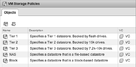
After the VM Storage Policy feature is enabled, a new area appears on the Summary tab for a VM that shows compliance or noncompliance with the assigned VM storage policy. For a VM that does not have a storage policy assigned—and we'll show you how to assign one shortly—the box is empty, like the one shown in Figure 6.61.
Perform these steps to assign a VM storage policy to a VM:
- In the vSphere Web Client, navigate to either the Hosts And Clusters view or the VMs And Templates view.
- Right-click a VM from the inventory panel and select Edit Settings.
- In the Edit Settings dialog box, click the arrow next to the virtual hard disk(s).
- From the drop-down list under VM Storage Policy, select the VM storage policy you want to assign to the VM's configuration and configuration-related files.
- For each virtual disk listed, select the VM storage policy you want associated with it.
Figure 6.62 shows a VM with a VM storage policy assigned to virtual hard disk 1.
FIGURE 6.60 The Enable VM Storage Policies dialog box shows the current status of VM policies and licensing compliance for the feature.
FIGURE 6.61 This VM does not have a VM storage policy assigned yet.
- Click OK to save the changes to the VM and apply the storage policy.
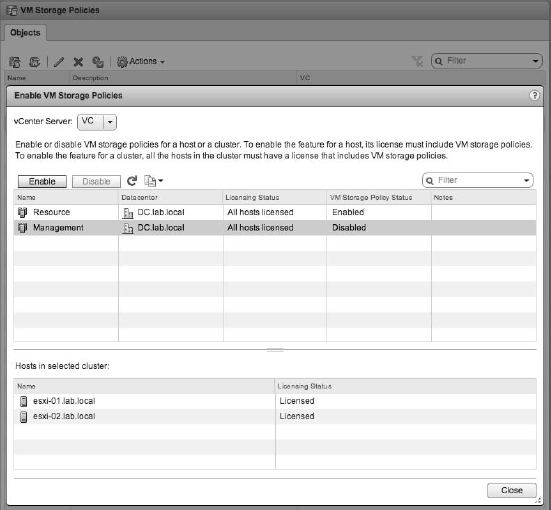
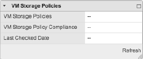
After a VM storage policy is assigned, this area will show the compliance (or noncompliance) of the VM's current storage with the assigned storage policy, as in Figure 6.63 and Figure 6.64.
FIGURE 6.62 Each virtual disk can have its own VM storage policy, so you tailor VM storage capabilities on a per-virtual disk basis.
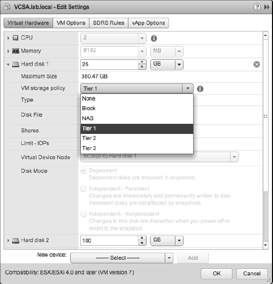
FIGURE 6.63 The storage capabilities specified in this VM storage policy don't match the capabilities of the VM's current storage location.
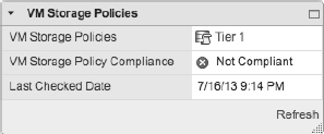
FIGURE 6.64 This VM's current storage is compliant with its assigned VM storage policy.
Figure 6.63 and Figure 6.64 also show the date and time of the last compliance check. Note that you can force a compliance check by clicking the Refresh hyperlink.
When we discuss creating VMs and adding virtual disks to a VM in Chapter 9, we'll revisit the concept of policy-driven storage and VM storage policies.
In addition to the various methods we've shown you so far for accessing storage from a VM, there's still one method left: using an in-guest iSCSI initiator.
USING IN-GUEST ISCSI INITIATORS
We mentioned in the section “Working with Raw Device Mappings” that RDMs were not the only way to present storage devices directly to a VM. You can also use an in-guest iSCSI initiator to bypass the hypervisor and access storage directly.
The decision whether to use in-guest iSCSI initiators will depend on numerous factors, including, but not limited to, your storage configuration (does your array support iSCSI?), your networking configuration and policy (do you have enough network bandwidth to support the additional iSCSI traffic on the VM-facing networks?), your application needs (do you have applications that need or are specifically designed to work with in-guest iSCSI initiators, or applications that need RDMs that could work with in-guest iSCSI initiators instead?), consolidation target (can you afford the extra CPU and memory overhead in the VMs as a result of using an in-guest iSCSI initiator?), and your guest OS (is there a software iSCSI initiator for your particular guest OS?).
Should you decide to use an in-guest iSCSI initiator, keep in mind the following tips:
- The storage that you access via the in-guest initiator will be separate from the NFS and VMFS datastores you'll use for virtual disks. Keep this in mind so that you can plan your storage configuration accordingly.
- You will be placing more load and more visibility on the VM networks because all iSCSI traffic will bypass the hypervisor. You'll also be responsible for configuring and supplying redundant connections and multipathing separately from the configuration you might have supplied for iSCSI at the hypervisor level. This could result in a need for more physical NICs in your server than you had planned.
- If you are using 10 Gigabit Ethernet, you might need to create a more complex QoS/Network I/O Control configuration to ensure that the in-guest iSCSI traffic is appropriately prioritized.
- You'll lose Storage vMotion functionality for storage accessed via the in-guest iSCSI initiator because the hypervisor is not involved.
- For the same reason, vSphere snapshots would not be supported for in-guest iSCSI initiator–access storage.
As with so many different areas in vSphere, there is no absolute wrong or right choice, only the correct choice for your environment. Review the impact of using iSCSI initiators in the guest OSes, and if it makes sense for your environment, proceed as needed.
THIN PROVISIONING: SHOULD YOU DO IT IN THE ARRAY OR IN VMWARE?
The general answer is that both are right.
If your array supports thin provisioning, it's generally more efficient to use array-level thin provisioning in most operational models. If you thick provision at the LUN or file system level, there will always be large amounts of unused space until you start to get it highly utilized, unless you start small and keep extending the datastore, which operationally is heavyweight.
Also, when you use thin-provisioning techniques at the array level using NFS or block storage, you always benefit. In vSphere, the common default virtual disk types—both thin and flat (with the exception of thick provisioned, which in vSphere is used far more rarely)—are friendly to storage-array-level thin provisioning since they don't pre-zero the files.
Thin provisioning also tends to be more efficient the larger the scale of the thin pool. On an array, this construct (often called a pool) tends to be larger than a single datastore and therefore more efficient because thin provisioning is more efficient at larger scales of thinly provisioned objects in the oversubscribed pool.
One other benefit of thin provisioning on the array, which is sometimes overlooked, is the extra capacity available for nonvirtual storage. When you're thin provisioning within vSphere only, the VMFS datastore takes the entire datastore capacity on the array, even if the datastore itself has no VMs stored within it.
Is there a downside to thin on thin? Not really, if you are able and willing to carefully monitor usage at both the vSphere layer and the storage layer. Use vSphere or third-party usage reports in conjunction with array-level reports, and set thresholds with notification and automated action on both the vSphere layer and the array level, if your array supports that. (See Chapter 13 for more information on creating alarms to monitor datastores.) Why? Even though vSphere 5.0 added thin-provisioning awareness and support, thin provisioning still needs to be carefully managed for out-of-space conditions because you are oversubscribing an asset that has no backdoor. Unlike the way VMware oversubscribes guest memory that can use VM swap if needed, if you run out of actual capacity for a datastore, the VMs on that datastore will be affected. When you use thin on thin, it can be marginally more efficient but can accelerate the transition to oversubscription and an outage.
An example here is instructive. If the total amount of provisioned space at the virtual disk layer in a datastore is 500 GB with thick virtual disks, then the datastore needs to be at least 500 GB in size, and therefore the LUN or NFS exported file system would need to look as if it were at least 500 GB in size. Now, those thick virtual disks are not actually using 500 GB; imagine that they have 100 GB of used space, and the remainder is empty. If you use thin provisioning at the storage array level, you provision a LUN or file system that is 500 GB, but only 100 GB in the pool is used. The space used cannot exceed 500 GB, so monitoring is needed only at the storage layer.
Conversely, if you use thin virtual disks, technically the datastore needs to be only 100 GB in size. The exact same amount of storage is being used (100 GB), but clearly there is a possibility of quickly needing more than 100 GB since the virtual disks could grow up to 500 GB without any administrative action—with only the VMs writing more data in their guest OSes. Therefore, the datastore and the underlying storage LUN/file system must be monitored closely, and the administrator must be ready to respond with more storage on the array and grow the datastore if needed.
There are only two exceptions to the “always thin provision at the array level if you can” guideline. The first is in the most extreme performance use cases, because the thin-provisioning architectures generally have a performance impact (usually marginal—and this varies from array to array) compared to a traditional thick-storage configuration. The second is large, high-performance RDBMS storage objects when the amount of array cache is significantly smaller than the database; ergo, the actual backend spindles are tightly coupled to the host I/O. These database structures have internal logic that generally expects I/O locality, which is a fancy way of saying that they structure data expecting the on-disk structure to reflect their internal structure. With very large array caches, the host and the backend spindles with RDBMS-type workloads can be decoupled, and this consideration is irrelevant. These two cases are important but rare. “Always thin provision at the array level if you can” is a good general guiding principle.
In the last section of this chapter, we'll pull together everything you've learned in the previous sections and summarize with some recommended practices.
Leveraging SAN and NAS Best Practices
After all the discussion of configuring and managing storage in vSphere environments, these are the core principles:
- Pick a storage architecture for your immediate and midterm scaling goals. Don't design for extreme growth scenarios. You can always use Storage vMotion to migrate up to larger arrays.
- Consider using VMFS and NFS together; the combination provides a great deal of flexibility.
- When sizing your initial array design for your entire vSphere environment, think about availability, performance (IOPS, MBps, latency), and then capacity—always together and generally in that order.
The last point in the previous list cannot be overstated. People who are new to storage tend to think primarily in the dimension of storage capacity (TB) and neglect availability and performance. Capacity is generally not the limit for a proper storage configuration. With modern large-capacity disks (300 GB+ per disk is common) and capacity reduction techniques such as thin provisioning, deduplication, and compression, you can fit a lot on a very small number of disks. Therefore, capacity is not always the driver of efficiency.
To make this clear, an example scenario will help. First, let's work through the capacity-centered planning dynamic:
- You determine you will have 150 VMs that are each 50 GB in size.
- This means that at a minimum, if you don't apply any special techniques, you will need 7.5 TB (150 × 50 GB). Because of extra space for vSphere snapshots and VM swap, you assume 25 percent overhead, so you plan 10 TB of storage for your vSphere environment.
- With 10 TB, you could fit that on approximately 13 large 1 TB SATA drives (assuming a 10+2 RAID 6 and one hot spare).
- Thinking about this further and trying to be more efficient, you determine that while the virtual disks will be configured to be 50 GB, on average they will need only 20 TB, and the rest will be empty, so you can use thin provisioning at the vSphere or storage array layer. Using this would reduce the requirement to 3 TB, and you decide that with good use of vSphere managed datastore objects and alerts, you can cut the extra space down from 25 percent to 20 percent. This reduces the requirement down to 3.6 TB.
- Also, depending on your array, you may be able to deduplicate the storage itself, which has a high degree of commonality. Assuming a conservative 2:1 deduplication ratio, you would then need only 1.5 TB of capacity—and with an additional 20 percent for various things, that's 1.8 TB.
- With only 1.8 TB needed, you could fit that on a very small 3+1 RAID 5 using 750 GB drives, which would net 2.25 TB.
This would be much cheaper, right? Much more efficient, right? After all, we've gone from 13 1 TB spindles to 4 750 GB spindles.
It's not that simple. This will be clear going through this a second time, but this time work through the same design with a performance-centered planning dynamic:
- You determine you will have 150 VMs (the same as before).
- You look at their workloads, and although they spike at 200 IOPS, they average at 50 IOPS, and the duty cycle across all the VMs doesn't seem to spike at the same time, so you decide to use the average.
- You look at the throughput requirements and see that although they spike at 200 MBps during a backup, for the most part, they drive only 3 MBps. (For perspective, copying a file to a USB 2 memory stick can drive 12 MBps—so this is a small amount of bandwidth for a server.) The I/O size is generally small—in the 4 KB size.
- Among the 150 virtual purpose machines, while most are general-purpose servers, there are 10 that are “big hosts” (for example, Exchange servers and some SharePoint backend SQL Server machines) that require specific planning, so you put them aside to design separately using the reference architecture approach. The remaining 140 VMs can be characterized as needing an average of 7,000 IOPS (140 × 50 IOPS) and 420 MBps of average throughput (140 × 3 MBps).
- Assuming no RAID losses or cache gains, 7,000 IOPS translates to the following:
- 39 15K RPM Fibre Channel/SAS drives (7,000 IOPS/180 IOPS per drive)
- 59 10K RPM Fibre Channel/SAS drives (7,000 IOPS/120 IOPS per drive)
- 87 5,400 RPM SATA drives (7,000 IOPS/80 IOPS per drive)
- 7 enterprise flash drives (7,000 IOPS/1000 IOPS per drive)
- Assuming no RAID losses or cache gains, 420 MBps translates into 3,360 Mbps. At the array and the ESXi hosts layers, this will require the following:
- Two 4 Gbps Fibre Channel array ports (although it could fit on one, you need two for high availability).
- Two 10 GbE ports (though it could fit on one, you need two for high availability).
- Four 1 GbE ports for iSCSI or NFS. NFS will require careful multi-datastore planning to hit the throughput goal because of how it works in link aggregation configurations. iSCSI will require careful multipathing configuration to hit the throughput goal.
- If using block devices, you'll need to distribute VMs across datastores to design the data-stores and backing LUNs themselves to ensure that they can support the IOPS of the VMs they contain so the queues don't overflow.
- It's immediately apparent that the SATA drives are not ideal in this case (they would require 87 spindles!). Using 300 GB 15K RPM drives (without using enterprise flash drives), at a minimum you will have 11.7 TB of raw capacity, assuming 10 percent RAID 6 capacity loss (10.6 TB usable). This is more than enough to store the thickly provisioned VMs, not to mention their thinly provisioned and then deduplicated variations.
- Will thin provisioning and deduplication techniques save capacity? Yes. Could you use that saved capacity? Maybe, but probably not. Remember, we've sized the configuration to meet the IOPS workload—unless the workload is lighter than we measured or the additional workloads you would like to load on those spindles generate no I/O during the periods the VMs need it. The spindles will all be busy servicing the existing VMs, and additional workloads will increase the I/O service time.
What's the moral of the story? That thin provisioning and data deduplication have no usefulness? That performance is all that matters?
No. The moral of the story is that to be efficient you need to think about efficiency in multiple dimensions: performance, capacity, power, operational simplicity, and flexibility. Here is a simple five-step sequence you can use to guide the process:
- Look at your workload, and examine the IOPS, MBps, and latency requirements.
- Put the outliers to one side, and plan for the average.
- Use reference architectures and a focused plan to design a virtualized configuration for the outlier heavy workloads.
- Plan first on the most efficient way to meet the aggregate performance workloads.
- Then, by using the performance configuration developed in step 4, back into the most efficient capacity configuration to hit that mark. Some workloads are performance bound (ergo, step 4 is the constraint), and some are capacity bound (ergo, step 5 is the constraint).
Let's quantify all this learning into applicable best practices:
When thinking about performance
- Do a little engineering by simple planning or estimation. Measure sample hosts, or use VMware Capacity Planner to profile the IOPS and bandwidth workload of each host that will be virtualized onto the infrastructure. If you can't measure, at least estimate. For virtual desktops, estimate between 5 and 20 IOPS. For light servers, estimate 50 to 100 IOPS. Usually, most configurations are IOPS bound, not throughput bound, but if you can, measure the average I/O size of the hosts (or again, use Capacity Planner). Although estimation can work for light server use cases, for heavy servers, don't ever estimate—measure them. It's so easy to measure, it's absolutely a “measure twice, cut once” case, particularly for VMs you know will have a heavy workload.
- For large applications (Exchange, SQL Server, SharePoint, Oracle, MySQL, and so on), the sizing, layout, and best practices for storage for large database workloads are not dissimilar to physical deployments and can be a good choice for RDMs or VMFS volumes with no other virtual disks. Also, leverage joint-reference architectures available from VMware and the storage vendors.
- Remember that the datastore will need to have enough IOPS and capacity for the total of all the VMs. Just remember 80 to 180 IOPS per spindle, depending on spindle type (refer to the Disks item in the list of elements that make up a shared storage array in the section “Defining Common Storage Array Architectures” earlier in this chapter), to support the aggregate of all the VMs in it. If you just add up all the aggregate IOPS needed by the sum of the VMs that will be in a datastore, you have a good approximation of the total. Additional I/Os are generated by the zeroing activity that occurs for thin and flat (but not thick, which is pre-zeroed up front), but this tends to be negligible. You lose some IOPS because of the RAID protection, but you know you're in the ballpark if the number of spindles supporting the datastore (via a file system and NFS or a LUN and VMFS) times the number of IOPS per spindle is more than the total number of IOPS needed for the aggregate workload. Keep your storage vendor honest and you'll have a much more successful virtualization project!
- Cache benefits are difficult to predict; they vary a great deal. If you can't do a test, assume they will have a large effect in terms of improving VM boot times with RDBMS environments on VMware but almost no effect otherwise, so plan your spindle count cautiously.
When thinking about capacity
- Consider not only the VM disks in the datastores but also their snapshots, their swap, and their suspended state and memory. A good rule of thumb is to assume 25 percent more than from the virtual disks alone. If you use thin provisioning at the array level, oversizing the datastore has no downside because only what is necessary is actually used.
- There is no exact best practice datastore-sizing model. Historically, people have recommended one fixed size or another. A simple model is to select a standard guideline for the number of VMs you feel comfortable with in a datastore, multiply that number by the average size of the virtual disks of each VM, add the overall 25 percent extra space, and use that as a standardized building block. Remember, VMFS and NFS datastores don't have an effective limit on the number of VMs—with VMFS you need to consider disk queuing and, to a much lesser extent, SCSI reservations; with NFS you need to consider the bandwidth to a single datastore.
- Be flexible and efficient. Use thin provisioning at the array level if possible, and if your array doesn't support it, use it at the VMware layer. It never hurts (so long as you monitor), but don't count on it resulting in needing fewer spindles (because of performance requirements).
- If your array doesn't support thin provisioning but does support extending LUNs, use thin provisioning at the vSphere layer, but start with smaller VMFS volumes to avoid oversizing and being inefficient.
- In general, don't oversize. Every modern array can add capacity dynamically, and you can use Storage vMotion to redistribute workloads. Use the new managed datastore function to set thresholds and actions, and then extend LUNs and the VMFS datastores using the new vSphere VMFS extension capability, or grow NFS datastores.
When thinking about availability
- Spend the bulk of your storage planning and configuration time to ensure that your design has high availability. Check that array configuration, storage fabric (whether Fibre Channel or Ethernet), and NMP/MPP multipathing configuration (or NIC teaming/link aggregation and routing for NFS) are properly configured. Spend the effort to stay up to date with the interoperability matrices of your vendors and the firmware update processes.
- Remember, you can deal with performance and capacity issues as they come up nondisruptively (VMFS expansion/extends, array tools to add performance, and Storage vMotion). Something that affects the overall storage availability will be an emergency.
When deciding on a VM datastore placement philosophy, there are two common models: the predictive scheme and the adaptive scheme.
Predictive scheme
- Create several datastores (VMFS or NFS) with different storage characteristics, and label each datastore according to its characteristics.
- Locate each application in the appropriate RAID for its requirements by measuring the requirements in advance.
- Run the applications, and see whether VM performance is acceptable (or monitor the HBA queues as they approach the queue-full threshold).
- Use RDMs sparingly as needed.
Adaptive scheme
- Create a standardized datastore building-block model (VMFS or NFS).
- Place virtual disks on the datastore. Remember, regardless of what you hear, there's no practical datastore maximum number. The question is the performance scaling of the datastore.
- Run the applications and see whether disk performance is acceptable (on a VMFS data-store, monitor the HBA queues as they approach the queue-full threshold).
- If performance is acceptable, you can place additional virtual disks on the datastore. If it is not, create a new datastore and use Storage vMotion to distribute the workload.
- Use RDMs sparingly.
Our preference is a hybrid. Specifically, you can use the adaptive scheme coupled with (starting with) two wildly divergent datastore performance profiles (the idea from the predictive scheme), one for utility VMs and one for priority VMs.
Always read, follow, and leverage the key documentation:
- VMware's Fibre Channel and iSCSI SAN configuration guides
- VMware's HCL
- Your storage vendor's best practices/solutions guides
Sometimes the documents go out of date. Don't just ignore the guidance if you think it's incorrect; use the online community or reach out to VMware or your storage vendor to get the latest information.
Most important, have no fear!
Physical host and storage configurations have historically been extremely static, and the penalty of error in storage configuration from a performance or capacity standpoint was steep. The errors of misconfiguration would inevitably lead not only to application issues but to complex work and downtime to resolve. This pain of error has ingrained in administrators a tendency to overplan when it comes to performance and capacity.
Between the capabilities of modern arrays to modify many storage attributes dynamically and Storage vMotion (the ultimate “get out of jail free card”—including complete array replacement!), the penalty and risk are less about misconfiguration, and now the risk is more about oversizing or overbuying. You cannot be trapped with an underperforming configuration you can't change nondisruptively.
More important than any storage configuration or feature per se is to design a highly available configuration that meets your immediate needs and is as flexible to change as VMware makes the rest of the IT stack.
The Bottom Line
Differentiate and understand the fundamentals of shared storage, including SANs and NAS. vSphere depends on shared storage for advanced functions, cluster-wide availability, and the aggregate performance of all the VMs in a cluster. Designing a high-performance and highly available shared storage infrastructure is possible on Fibre Channel, FCoE, and iSCSI SANs and is possible using NAS; in addition, it's available for midrange to enterprise storage architectures. Always design the storage architecture to meet the performance requirements first, and then ensure that capacity requirements are met as a corollary.
Master It Identify examples where each of the protocol choices would be ideal for different vSphere deployments.
Master It Identify the three storage performance parameters and the primary determinant of storage performance and how to quickly estimate it for a given storage configuration.
Understand vSphere storage options. vSphere has three fundamental storage presentation models: VMFS on block, RDM, and NFS. The most flexible configurations use all three, predominantly via a shared-container model and selective use of RDMs.
Master It Characterize use cases for VMFS datastores, NFS datastores, and RDMs.
Master It If you're using VMFS and there's one performance metric to track, what would it be? Configure a monitor for that metric.
Configure storage at the vSphere layer. After a shared storage platform is selected, vSphere needs a storage network configured. The network (whether Fibre Channel or Ethernet based) must be designed to meet availability and throughput requirements, which are influenced by protocol choice and vSphere fundamental storage stack (and in the case of NFS, the network stack) architecture. Proper network design involves physical redundancy and physical or logical isolation mechanisms (SAN zoning and network VLANs). With connectivity in place, configure LUNs and VMFS datastores and/or NFS exports/NFS datastores using the predictive or adaptive model (or a hybrid model). Use Storage vMotion to resolve hot spots and other non-optimal VM placement.
Master It What would best identify an oversubscribed VMFS datastore from a performance standpoint? How would you identify the issue? What is it most likely to be? What would be two possible corrective actions you could take?
Master It A VMFS volume is filling up. What are three possible nondisruptive corrective actions you could take?
Master It What would best identify an oversubscribed NFS volume from a performance standpoint? How would you identify the issue? What is it most likely to be? What are two possible corrective actions you could take?
Configure storage at the VM layer. With datastores in place, create VMs. During the creation of the VMs, place VMs in the appropriate datastores, and employ selective use of RDMs but only where required. Leverage in-guest iSCSI where it makes sense, but understand the impact to your vSphere environment.
Master It Without turning the machine off, convert the virtual disks on a VMFS volume from thin to thick (eagerzeroedthick) and back to thin.
Master It Identify where you would use a physical compatibility mode RDM, and configure that use case.
Leverage best practices for SAN and NAS storage with vSphere. Read, follow, and leverage key VMware and storage vendors' best practices/solutions guide documentation. Don't oversize up front, but instead learn to leverage VMware and storage array features to monitor performance, queues, and backend load—and then nondisruptively adapt. Plan for performance first and capacity second. (Usually capacity is a given for performance requirements to be met.) Spend design time on availability design and on the large, heavy I/O VMs, and use flexible pool design for the general-purpose VMFS and NFS datastores.
Master It Quickly estimate the minimum usable capacity needed for 200 VMs with an average VM size of 40 GB. Make some assumptions about vSphere snapshots. What would be the raw capacity needed in the array if you used RAID 10? RAID 5 (4+1)? RAID 6 (10+2)? What would you do to nondisruptively cope if you ran out of capacity?
Master It Using the configurations in the previous question, what would the minimum amount of raw capacity need to be if the VMs are actually only 20 GB of data in each VM, even though they are provisioning 40 GB and you used thick on an array that didn't support thin provisioning? What if the array did support thin provisioning? What if you used Storage vMotion to convert from thick to thin (both in the case where the array supports thin provisioning and in the case where it doesn't)?
Master It Estimate the number of spindles needed for 100 VMs that drive 200 IOPS each and are 40 GB in size. Assume no RAID loss or cache gain. How many if you use 500 GB SATA 7200 RPM? 300 GB 10K Fibre Channel/SAS? 300 GB 15K Fibre Channel/SAS? 160 GB consumer-grade SSD? 200 GB Enterprise Flash?