
8
Third-Order Unsteady Adaptation
The quest for efficiency leads to combine mesh adaptation with higher order accuracy. This chapter presents a first attempt toward such a combination. A third-order accurate Central Essentially Non-Oscillatory (CENO) approximation is chosen for the demonstration. An a priori error analysis is developed. Then, using a least square projection of the error to a metric-based error reduces the mesh adaptation goal-oriented problem to the optimization of a metric. The numerical illustration concerns nonlinear sound propagation.
8.1. Introduction
Second-order mesh-adaptative approaches bring a good level of safety in the obtention of converging approximate solutions. But these solutions finally obtained are in best case second-order converging to the exact solution. On the other side, high-order solutions are much more efficient when they converge at high order, but often, convergence at high order is not obtained, either because mesh is not sufficient, or because the solution is singular or has stiff variations. Therefore, the Graal for getting accuracy and safety is to combine mesh adaptation and higher order approximations. In order to present a method combining both, we shall choose a higher order approximation. The recent investigations with unstructured meshes concern mainly discontinuous Galerkin (DG) approximations. DG is quite different (data structures, etc.) from the approximations considered in this book. Also, we are interested by singularities, for example, shocks, and, depending on the location of the shock in the mesh, the capture of the discontinuity by DG can be of good or less good quality. These two problems are avoided by a method like ENO. In this chapter, we consider mesh adaptation for a third-order accurate CENO approximation based on a quadratic polynomial reconstruction (then CENO2), which is used to approximate the unsteady Euler equations. This scheme is inspired by the CENO proposition of Ivan and Groth (2014; see also Yan and Ollivier-Gooch 2017). We transpose it beforehand into a vertex formulation. Because the third-order upwind scheme is rather dissipative, a modification is proposed in order to improve the approximation properties of the scheme according to the above criteria, focusing on its advective performances. As for the original unstructured CENO scheme (Charest et al. 2015), the new scheme is third-order accurate on irregular unstructured meshes.
Section 8.2 examines how to evaluate reconstruction errors. Section 8.3 presents shortly the numerical scheme, which has been designed for our investigation. Section 8.4 develops an error estimate based on the PDE, in order to build a goal-oriented mesh adaptation algorithm. The resulting a priori error analysis is a kind of dual of the a posteriori analysis of Barth and Larson (2002). Section 8.5 considers the extension of a metric-based adaptation method to take into account the cubic reconstruction error. Cao (2007b) proposes a first approximation of this error with stretching directions. In the present chapter, we propose to replace the application of the third derivative tensor to a mesh size vector by the power 3/2 of the application of a pseudo-Hessian second-order tensor to this mesh size. The optimal metric is defined in section 8.6. The practical approach for an unsteady model is considered in section 8.7. For solving the resulting mesh optimality system, we discretize it and apply the global unsteady fixed point Algorithm 8.1. In section 8.8, the unsteady method is applied to an acoustic propagation benchmark and compared with previous approaches.
8.2. Higher order interpolation and reconstruction
Most high-order approximation schemes like DG (Bassi and Rebay 1997; Cockburn et al. 2000; Cockburn 2001; Shu and Cockburn 2001), ENO (Engquist et al. 1986; Barth and Frederickson 1990; Lafon and Abgrall Novembre 1993; Groth and Ivan 2011) or distributive schemes (Abgrall 2006) use kth-order interpolation or reconstruction and are k-exact in the sense that polynomial solutions of degree k are approximated without any error by such schemes. Interpolation and reconstruction are two approximation mappings, the errors of which need to be analyzed. Most analyses are inspired by the Bramble–Hilbert principle, stating that an approximation that is exact for kth-order polynomial is a (k +1)th-order accurate approximation. Demonstrations can be found in the fundamental paper (Ciarlet and Raviart 1972). Later, when considering reconstruction-based schemes (see Harten and Chakravarthy 1991), the authors referred to the Taylor series. A re-visitation in Abgrall (1992) establishes the link with Ciarlet and Raviart (1972). Interpolation errors are used for building adaptation criteria in Huang (2005). Several metrics are derived from the Hessians of each partial derivative. Then the metrics are intersected. A similar idea is presented in Hecht (2008). Intersections of metrics do not easily produce optimal meshes. They often result in a too severe anisotropy loss. A true asymptotic extension is proposed in Cao (2005, 2008). We also refer to Mirebeau (2010) for similar ideas. A singular Sylvester decomposition is applied in Mbinky (2013).
Let us focus in this section on the estimation of the reconstruction error. Given a function with sufficiently smooth u defined on a bounded domain Ω limited by a continuous boundary, given a tesselation of Ω into cells Ci of centroids ci, and the array ![]() of means of u on cells Ci, we are interested by polynomials
of means of u on cells Ci, we are interested by polynomials ![]() of degree k built on any cell i and of same mean on cell i as u:
of degree k built on any cell i and of same mean on cell i as u:
where J(i) a set of cells close to cell Ci and ℓ holds for the usual multi-index notation, in 2D:

According to Harten and Chakravarthy (1991), for a sufficiently large neighborhood J(i) of cells around i,we have

where diameters of cells are less than h. Note that if we define the operator
then, as far as the J(i)’s are sufficiently large, Π is k-exact (mapping a kth-order polynomial in itself). In Abgrall (1992), the authors use a result from Ciarlet and Raviart (1972) to give a more accurate estimate in the Sobolev space Wm,p(Ω) equipped of the following norm and semi-norm: ![]()
It is written as
for a certain constant C and where ρ is related to the shape of cells and m is any integer such that 0 ≤ m ≤ k +1. This shows that the reconstruction error is, when k = 2, effectively expressed in terms of the third derivative of u.
A last remark is that in the case of a mean-square-based reconstruction, if the number of cells of the support is exactly the number of unknown coefficients, then the minimum of the least square functional is zero that shows (for a smooth function) that the reconstruction is equal to the initial function in one point of each neighboring cell; in other words, the reconstruction is an interpolation, the error of which is given by the Taylor expansion. In the general case, we do not have a precise estimate, and we choose to get inspired by the Taylor expansion and heuristically write our reconstruction error estimate as follows:
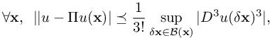
where ≼ holds for an inequality that holds for mesh size sufficiently small and where the δx describes the unit ball B(x) of local mesh sizes around x, as defined in definition 3.18.
8.3. CENO approximation for the 2D Euler equations
8.3.1. Model
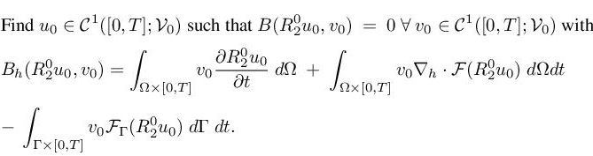
The unsteady 2D Euler equations in a geometrical bounded domain ![]() of boundary Γ can be written as
of boundary Γ can be written as
Here, V = L2(0,T; H1(Ω)) ∩ H1(0,T; L2(Ω)) and u = (u1, u2, u3, u4) hold for the conserved unknowns (density, moments components, energy) and ∇ · F = ![]() with
with
for the usual four Euler fluxes of mass, moments and energy. At right-hand side, we have an integral of the various boundary fluxes FΓ for various boundary conditions, which we do not need to detail here. Defining

the variational formulation is written as follows:
8.3.2. CENO formulation
We choose a reconstruction-based finite-volume method, being inspired by the unlimited version of the reconstruction technique of Barth (1993) and the CENO methods. Concerning the location of the nodes with respect to the mesh elements, we prefer to minimize the number of unknowns with respect to a given mesh; therefore we keep the vertex-centered location already used in this book for second-order anisotropic (Hessian-based or goal-oriented) mesh adaptation (Chapter 5 of Volume 1 and Chapters 2, 4 and 7 of Volume 2). For a more detailed description of the CENO approach presented here, see Ouvrard et al. (2009). Its main features are as follows: (a) vertex centered, (b) dual median cells around the vertex, (c) a single mean square quadratic reconstruction for each dual cell, (d) Roe approximate Riemann solver for stabilization and (e) explicit multi-stage time-stepping. The computational domain is divided in triangles and in a dual tesselation in cells, each cell Ci being built around a vertex i, with limits following sections of triangle medians (Figure 8.1). We define the discrete space V0 of functions of V, which are constant on any dual cell Ci. Let us define a discrete reconstruction operator![]() The operator
The operator ![]() reconstructs a function of V0 in each cell Ci under the form of a second-order polynomial:
reconstructs a function of V0 in each cell Ci under the form of a second-order polynomial: ![]() Given the means
Given the means ![]() of u0 on cells
of u0 on cells ![]() is defined by the
is defined by the ![]() such that
such that
where ![]() stands for the mean of
stands for the mean of ![]() on cell j, and the set of neighboring cells is taken sufficiently large for an accurate quadratic reconstruction (see Figure 8.1).
on cell j, and the set of neighboring cells is taken sufficiently large for an accurate quadratic reconstruction (see Figure 8.1).
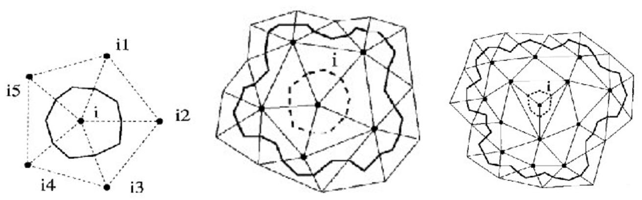
Figure 8.1. Dual cell and two reconstruction molecules
For the Euler model [8.4], the semi-discretized CENO scheme is written as follows:
In [8.5], the term ![]() needs to be defined, since
needs to be defined, since ![]() is discontinuous at cells interfaces. Taking v0 as a characteristic function of cell Ci, we get the following finite volume formulation:
is discontinuous at cells interfaces. Taking v0 as a characteristic function of cell Ci, we get the following finite volume formulation:

or, (using ![]() ),
),

Neither the discrete divergence ∇h· nor the CENO approximation is defined by the definition of the reconstruction. Indeed, the reconstruction performed in each cell produces a global field, which is generally discontinuous at cell interfaces ∂Ci ∩ ∂Cj (see Figure 8.2). In order to fix an integration value at the interface, we can consider an arithmetic mean of the fluxes values for the two reconstruction values:
where ![]() holds for the value at cell boundary of the reconstructed
holds for the value at cell boundary of the reconstructed ![]() on cell Ci. The above mean is applied on the four Gauss integration points (gα,α = 1, 4) (two per interface segment, see Figure 8.2) necessary for an exact integration of quadratic polynomials. Then the accurate definition of Bh is as follows:
on cell Ci. The above mean is applied on the four Gauss integration points (gα,α = 1, 4) (two per interface segment, see Figure 8.2) necessary for an exact integration of quadratic polynomials. Then the accurate definition of Bh is as follows:

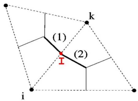
Figure 8.2. Sketch of the interface ∂Ci ∩ ∂Ck between cell Ci and cell Ck. It is made of two segments (1) and (2) joining mid-edge I and triangles centroid. Flux integration on (1) (respectively, (2)) will rely on two Gauss integration points. For a color version of this figure, see www.iste.co.uk/dervieux/meshadaptation2
The restriction of Bh to smooth function is B and for the continuous solution u satisfies:
It remains to define a time discretization for [8.6]. We apply the standard explicit Runge-Kutta (RK4) time advancing. With the above central-differenced [8.7] spatial quadrature, this formulation produces a central-differenced numerical approximation, which is third-order accurate. However, in a nonlinear setting or on irregular unstructured meshes, it cannot be used due to a lack of stability.
8.3.3. Vertex-centered low dissipation CENO2
Scheme [8.6] is usually combined with an approximate Riemann solver instead of the formulation [8.7] proposed in the previous section. This latter option produces the usual upwind-CENO scheme, which enjoys a rather good nonlinear stability, but shows in applications a relatively large dissipation error. Indeed, its 1D analysis put in evidence a dominant dissipation error term of weight Δx3 and similar to the fourth spatial derivative of the unknown solution, as it is the case of usual second-order approximations. In contrast, using a four-degree reconstruction would produce an approximation scheme involving solely a dissipation by sixth spatial derivative, in Δx5, much smaller. In the rest of this chapter, we shall use a low-dissipation version introduced in Carabias et al. (2011). The CENO with central differencing on integration points for fluxes is stabilized by the use on each edge ij of approximates polynomial 1D interpolations in the direction of ij. We refer to Carabias et al. (2011) for details. The reader just needs to know that the accuracy is impressively improved as sketched in Figure 8.3, which compares the advection of a Gaussian profile for the upwind CENO and the low-dissipation one. Both schemes are third-order accurate and the error analysis can be performed for both schemes without considering the low-dissipation modification.
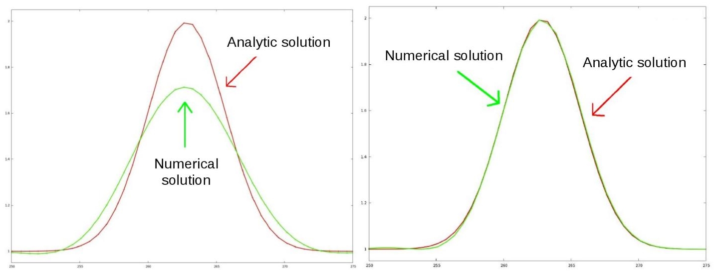
Figure 8.3. Improvement of the CENO scheme for the advection of a 2D Gauss-shaped concentration through 400 space intervals. Left: Comparison of the upwind third-order accurate CENO solution with the analytic solution. Right: Comparison of the improved (third-order accurate) CENO scheme with the analytic solution. For a color version of this figure, see www.iste.co.uk/dervieux/meshadaptation2
8.4. Error analysis
In the present work, we do not consider time discretization errors. For explicit high-order time-advancing subject to a Courant-type condition, some argument for discarding the time-error analysis of advective models can be found in the Annex of Chapter 2 of this volume. We then concentrate on spatial errors. Furthermore, we do not analyze the corrections terms introduced in previous section. At least on regular meshes, these corrections terms are terms of higher order. The proposed a priori analysis is in some manner the dual of the a posteriori analysis proposed by Barth and Larson (2002). Let j(u) = (g, u) be the scalar output, which we want to accurately compute, where u is the solution of the continuous system [8.4]. We concentrate on the reduction, by mesh adaptation, of the following error:
where g is function of L2(Ω) and u0 the discrete solution of [8.6]. The projection π0 is defined by
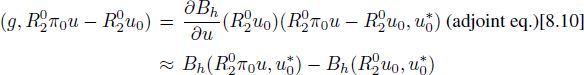
The adjoint state ![]() is the solution of Bh (defined in [8.5]):
is the solution of Bh (defined in [8.5]):
Then we can write, successively,
and then
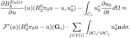
For the case of Euler equations, the previous error estimate is written as
with
with the sum applied for all dual cell Ci of the mesh. Since, as in Loseille et al. (2007), we do not consider the adaptation of boundary mesh, we discard the boundary terms:

that is,
Let us examine the ingredients of the RHS integrand. First, ![]() is constant by cell, with discontinuities at cell interface of amplitude of order of mesh size. The Jacobian F′(u) is smooth. The reconstruction error
is constant by cell, with discontinuities at cell interface of amplitude of order of mesh size. The Jacobian F′(u) is smooth. The reconstruction error ![]() is discontinuous at cell interfaces, but for a u smooth, the amplitude of this discontinuity is of order the third power of mesh size. Then
is discontinuous at cell interfaces, but for a u smooth, the amplitude of this discontinuity is of order the third power of mesh size. Then
where Gi is the centroid of cell Ci. Thus,
We recognize inside the RHS the approximation of a gradient of ![]()
thus
As remarked in section 8.2, ![]() can be replaced by a smooth function of the local third derivatives and local mesh size (factor
can be replaced by a smooth function of the local third derivatives and local mesh size (factor ![]() can be discarded in the rest of the analysis):
can be discarded in the rest of the analysis):
For each flux component (r = 1, 8),
Then
with
with the notation F according to [8.3], and
It will be useful to write it as follows:
where T is the trilinear tensor:

Not surprisingly, the error is a third-order tensor in terms of the δx, measuring local mesh size. In order to apply a metric-based mesh adaptation, we shall convert the estimate in a pseudo-quadratic estimate.
8.5. Metric-based error estimate
Given a Riemannian metric ![]() parameterizing the mesh (Chapter 3 of Volume 1), the P1 interpolation error of a smooth (at least C2) function uq satisfies the following:
parameterizing the mesh (Chapter 3 of Volume 1), the P1 interpolation error of a smooth (at least C2) function uq satisfies the following:
where Huq is the Hessian of uq , and orthonormal directions ![]() and
and ![]() are eigenvectors of this Hessian and δxM a vector of
are eigenvectors of this Hessian and δxM a vector of ![]() such that
such that ![]() . This formulation permits the research of an optimal metric minimizing the linear interpolation error (Chapter 4 of Volume 1). We have to adapt this to a higher order interpolation/reconstruction. In Mbinky et al. (2012), the authors propose a general statement for an interpolation of arbitrary degree generalizing [8.14]. We prefer here a simpler option. In order to address our third-order mesh adaptation problem in a similar manner to the Hessian-based approach, we propose instead using T to define on each vertex i a pseudo-Hessian
. This formulation permits the research of an optimal metric minimizing the linear interpolation error (Chapter 4 of Volume 1). We have to adapt this to a higher order interpolation/reconstruction. In Mbinky et al. (2012), the authors propose a general statement for an interpolation of arbitrary degree generalizing [8.14]. We prefer here a simpler option. In order to address our third-order mesh adaptation problem in a similar manner to the Hessian-based approach, we propose instead using T to define on each vertex i a pseudo-Hessian ![]() in such a way that inside cell i we have (see [8.1])
in such a way that inside cell i we have (see [8.1])
In the continuous mesh model, the set of neighboring vertices j around a given vertex i is the surface of an ellipse centered on i and with small and large axis defined by the metric matrix M. One way to adjust the pseudo-Hessian ![]() consistently with the discrete context is to minimize by least square projection the deviation between the quadratic term and the trilinear one. The ball B(x) is approximated by considering any edge ij around i in the current mesh:
consistently with the discrete context is to minimize by least square projection the deviation between the quadratic term and the trilinear one. The ball B(x) is approximated by considering any edge ij around i in the current mesh:
with ![]() being the set of neighbors of i. Replacing then the trilinear estimate by the 3/2 power of the quadratic term, we get
being the set of neighbors of i. Replacing then the trilinear estimate by the 3/2 power of the quadratic term, we get
We consider now a way to find a metric field which minimizes this error term.
8.6. Optimal metric
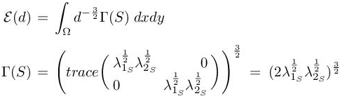
Because of the above transformation of the error estimate, we can consider the minimization of the following error functional derived from estimate [8.13]:
We then obtain
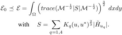
Matrix S(x) is a sum of symmetric positive definite matrices, thus ![]() . We now identify the optimal metric, Mopt = Mopt(N), among those having a prescribed total complexity N, which minimizes the above error. We proceed similarly to the second-order metric analysis (section 4.4 of this volume). To do so, we re-write [8.15] as
. We now identify the optimal metric, Mopt = Mopt(N), among those having a prescribed total complexity N, which minimizes the above error. We proceed similarly to the second-order metric analysis (section 4.4 of this volume). To do so, we re-write [8.15] as
Mesh stretching direction. We first prescribe, at each point x of the computational domain Ω, the adapted metric eigenvectors, that is, the representation of the direction of stretching of mesh, RMopt as aligned with the above error model, that is,
Mesh stretching length. Let us minimize the error at each point x of the computational domain for a prescribed mesh density dM. We derive that the best ratio of eigenvalues for M, that is, the representation of mesh stretching or anisotropy should uniformize the two components of the error. This means that the product
is made proportional to identity. It implies that
in which we have enforced ![]() With these definitions of
With these definitions of ![]() and
and ![]() weget
weget

Inside this restricted family of metrics, it remains to define the optimal metric density. Let us consider the set of metrics with a total number of vertices prescribed to N:
We now have to minimize the L1 norm of the error
with respect to d for a given number of nodes N. This means that
which implies that the derivative ![]() of integrand in E is constant and produces the optimal density
of integrand in E is constant and produces the optimal density

This completes the definition of the optimal metric:
8.7. From theory to practical application
The previous analysis sets the optimal metric problem as the solution of the following continuous optimality conditions:
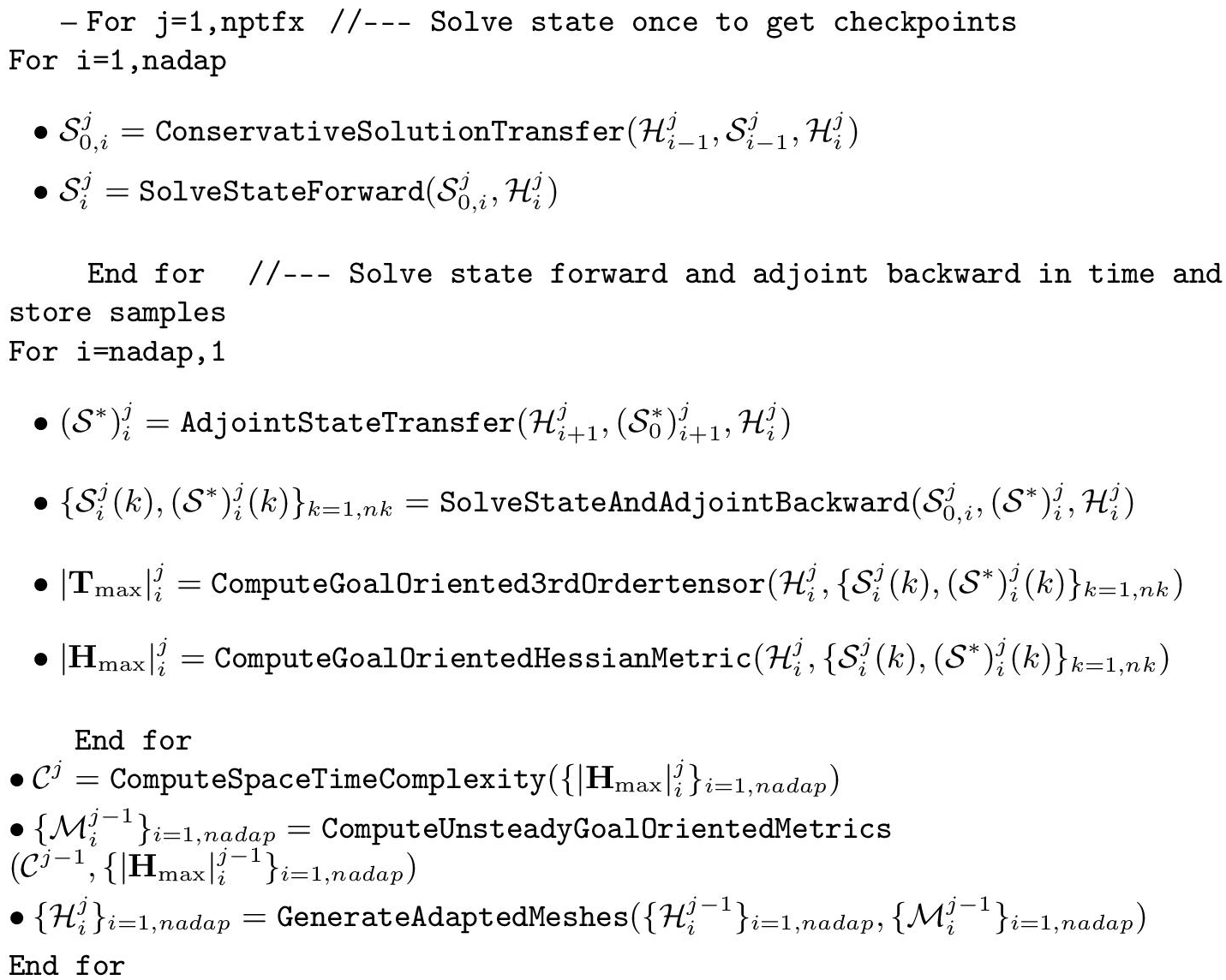
This system cannot be solved analytically and will be finally discretized. Not surprisingly, we choose the discrete state system as the one introduced previously. The adjoint is derived from its linearization. The last equation is discretized by recovering third-order derivatives by using a fourth-order reconstruction (like it would be done for a CENO3 scheme). Then, for each time step, the nonlinear iteration on the three equations of the optimality system provides an optimal metric and a unit mesh. In order to avoid to remesh too frequently, we adapt the Global Transient Fixed Point algorithm introduced in Chapter 7 of this volume and sketched in Figure 7.6. We keep its important features. The time interval has three embedded discretizations: (1) time sub-intervals ]ti,ti+1[ during which the mesh is frozen, (2) divisions ]ti,k, ti,k+1[ of these sub-intervals for checkpointing state solution to be re-used backward in time for solving the adjoint system and (3) an even finer discretization in the time-steps ]ti,k + mδt, ti,k +(m + 1)δt[ used to advance in time. For each subinterval nadap, each maximal metric ![]() is computed from the different variables and different time levels of the subinterval by applying the metric intersection defined in section 3.6.1 of Chapter 3 of Volume 1. We rewrite the adapted algorithm with the modification for third order in Algorithm 8.1. A crucial criterion for evaluating a mesh adaptation method is its a priori/theoretical convergence order in terms of used degrees of freedom. Similarly, the evaluation of a computation should also rely on numerical convergence order, which should be preferably close to the theoretical one. A detailed discussion of the convergence of the global transient fixed point is presented in section 2.9.2 of Volume 1. According to lemma 2.12, the space-time theoretical order (i.e. in terms of space and time degrees of freedom) is for an arbitrary flow (possibly with singularities) limited to 9/5 in 2D and 2 in 3D. In contrast, the space theoretical order, evaluated by considering solely spatial degrees of freedom maybe as high as the theoretical spatial truncation order. It can be measured by solely considering the mean number of vertices (for a fixed number of mesh-adaptation intervals).
is computed from the different variables and different time levels of the subinterval by applying the metric intersection defined in section 3.6.1 of Chapter 3 of Volume 1. We rewrite the adapted algorithm with the modification for third order in Algorithm 8.1. A crucial criterion for evaluating a mesh adaptation method is its a priori/theoretical convergence order in terms of used degrees of freedom. Similarly, the evaluation of a computation should also rely on numerical convergence order, which should be preferably close to the theoretical one. A detailed discussion of the convergence of the global transient fixed point is presented in section 2.9.2 of Volume 1. According to lemma 2.12, the space-time theoretical order (i.e. in terms of space and time degrees of freedom) is for an arbitrary flow (possibly with singularities) limited to 9/5 in 2D and 2 in 3D. In contrast, the space theoretical order, evaluated by considering solely spatial degrees of freedom maybe as high as the theoretical spatial truncation order. It can be measured by solely considering the mean number of vertices (for a fixed number of mesh-adaptation intervals).
Algorithm 8.1. Third-order global fixed-point
8.8. A numerical example: acoustic wave
A goal-oriented mesh adaptation algorithm is not designed to deliver an accurate or even simply convergent solution field since the adaptation effort is restricted to the best accuracy for the scalar output. If the scalar output for a transient simulation is a time integral, an interesting accuracy evaluation of a mesh-adaptive calculation concerns the integrand of this time integral. A successful mesh-adaptive calculation should show a third-order numerical convergence for a third-order accurate scheme. The experiment presented focus on the propagation of acoustic waves with an Euler model. It is a challenging simulation with a fixed but unstructured mesh for usual Euler schemes, which are generally too dissipative and dispersive. It is also a challenging problem for mesh adaptation since meshes cannot be regular and must follow traveling structures, which can go through the whole computational domain. We simulate the propagation of an acoustic wave between its emission and the time when the corresponding pressure fluctuation is recorded over a limited time interval with a microphone situated at some distance from the noise source. Not all sound waves will have influence on this record, and therefore, at each time level, only a part of the domain needs a fine mesh. And indeed, during these calculations, due to the effect of adjoint state, meshing concentrates only on a small part of the computational domain. We restrict to spatial accuracy and expect third-order convergence. In the two experiments which we describe, about 50 mesh-adaptation intervals (i.e. 50 meshes) are used in a time interval. The number of global fixed points iterations is 4. A typical wall time is 10 h on a laptop for the finest mesh.
The propagation considered is rather close to the one computed in section 7.7.1 of Chapter 7 of this volume, for which the Global Transient Fixed Point algorithm was combined with a second-order accurate scheme. For a sequence of adaptive meshes of 12K, 24K, 64K (mean size over the time interval), the numerical mesh convergence measured is 1.98. The challenge is now to get with the mesh adaptive algorithm a convergence numerical order close to 3. This computation is presented (in detail) in Carabias et al. (2018), in which unfortunately, because the computation was done on a not very fast laptop, the box is in this section two times smaller in order to have an easier case. We keep the same source term as [7.42] and the same output functional:
where p0 is the initial pressure. The mesh and pressure contours of two mesh-adaptative transient computations, a coarse one and a fine one are presented in Figure 8.4.
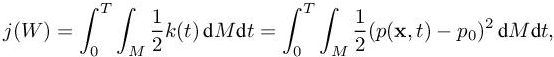
The numerical convergence order of the functional, is as expected, close to third order. But the method seems to provide also some superconvergence for some outputs. Indeed, let us analyze the convergence of the time-integrand k(t) of the functional
at some particular time t = t∗ for the different mesh-adaptive calculations. The variations of k are depicted in Figure 8.5. Numerical convergence order is measured on the maximum k(t∗) of k , reached for time close to t = 10.5. It is obtained (by solving equation [6.3] (Chapter 6 of Volume 1) for three consecutive mesh sizes, the mean mesh sizes being successively 1,500, 5,400, 11,000 and 21,000. For the three finer calculations, with mean mesh sizes of 5,400, 11,000 and 21,000 vertices, convergence order appears as equal to 2.71, a level much higher than second-order case of section 7.7.1 (for which the fine adapted mesh was two times finer) and close to the theoretical order 3 (see Table 8.1). The meshes are anisotropic with aspect ratio larger than 3 to 4 in regions of interest. The smaller mesh size for the different meshes (at different times) are of order of 5 × 10⁻⁴, which would be obtained with a uniform isotropic mesh of about 2 million vertices.
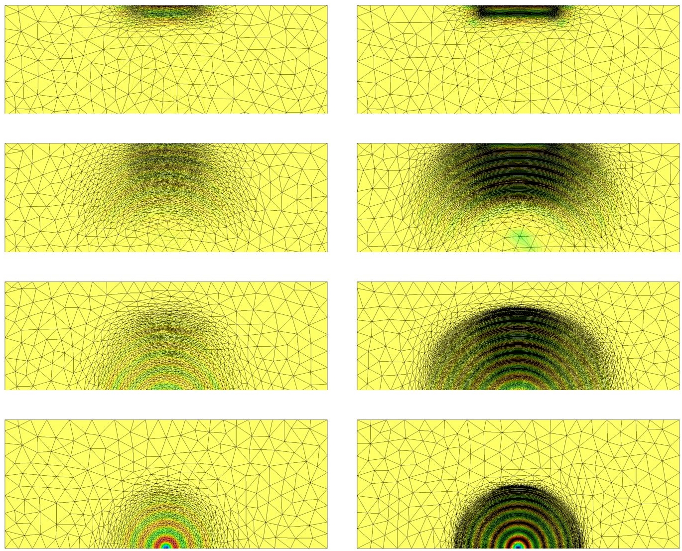
Figure 8.4. Acoustic waves traveling in a box from bottom (5th mesh in time) to top (20th mesh in time) with the coarse option (left, 1,500 vertices in the mean) and the finest option (right, 21,566 vertices in the mean). For a color version of this figure, see www.iste.co.uk/dervieux/meshadaptation2
Table 8.1. Noise propagation in a rectangular box: mesh convergence for the unsteady integrand
| Mean mesh size | Maximum close to T=10.5s | Observed convergence order |
|---|---|---|
| 2,775 | 6.893079.10−07 | |
| 5,403 | 7.235717.10−07 | |
| 10,696 | 7.431403.10−07 | 1.70 |
| 21,566 | 7.510065.10−07 | 2.71 |
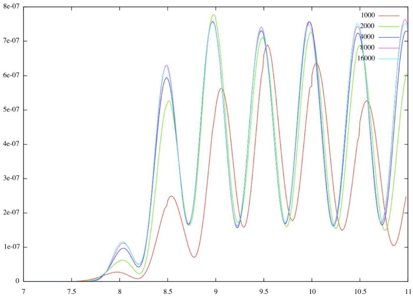
Figure 8.5. Noise propagation in a box: mesh convergence of the spatial integral k(t) (y-axis) as a function of time (x-axis). The lower curve “1000” corresponds to a mean mesh size of 1,500 vertices. The three other curves, almost undistinguishable, correspond to mean mesh sizes of 5,400, 11,000 and 21,000 vertices. For a color version of this figure, see www.iste.co.uk/dervieux/meshadaptation2
8.9. Conclusion
This chapter describes an a priori analysis of the error of a third-order accurate CENO scheme for the unsteady Euler equations. The proposed analysis expresses all distributed error terms as functions of reconstruction errors. It allows to predict the effect of a given mesh (mesh size, anisotropy) on the approximation error. An important simplification consists in projecting the estimate on a metric-based analysis because of least square projection. This allows for an anisotropic mesh adaptation relying on an optimal metric, and solving goal-oriented problematics. A convergence order of 2.71, much better than with second-order accurate adaptation, is obtained with less degrees of freedom.
8.10. Notes
More computational results can be found in Carabias et al. (2018).
Let us also mention that the numerical scheme used here has been extended to shock capturing in Carabias (2013).
Short review of higher order adaptation. As already remarked in the chapter, interpolation errors are used for building adaptation criteria in Huang (2005). Several metrics are derived from the Hessians of each partial derivative. Then the metrics are intersected. A similar idea is discussed in Hecht (2008). Intersections of metrics do not produce really optimal meshes. Further they often result in loosing anisotropy. A true asymptotic extension is proposed in Cao (2005, 2008; see also Cao 2007a,b). We also refer to Mirebeau (2010) for similar ideas. A singular Sylvester decomposition is applied in Mbinky (2013). Further proposals for adapting a local molecule to a higher order polynomial are given in Coulaud and Loseille (2016). A proposal for h-p adaptation by measuring the different terms of the Taylor series is studied in Dolejsi (2014), Dolejsi et al. (2018), Rangarajan et al. (2017) (using a continuous mesh model) and Rangarajan et al. (2018). Researcher using CENO-like schemes have derived adapted approaches (see Ivan and Groth 2007; Pagnutti and Ollivier-Gooch 2009; Ivan 2011; Ivan et al. 2014). Approaches relying on optimization are proposed for higher order in Yano et al. (2011), Darmofal et al. (2013) and Yano and Darmofal (2014).