
Chapter 11
Frailty Models
11.1 Introduction
The notion of frailty provides a useful way for modeling unobserved heterogeneity and associations in survival analysis. In its simplest form, frailty is an unobserved random proportionality factor that modifies the hazard function of an individual or related individuals. In essence, the frailty concept goes back to the work of Greenwood and Yule [1] on “accident proneness.” The notion of frailty itself was coined by Vaupel et al. [2] for univariate survival data, and the approach was substantially promoted by its extension to multivariate survival models by Clayton [3] on chronic disease incidence in families (without using the notion of frailty).
Frailty models are extensions of the proportional hazards Cox model [4], the most popular model in survival analysis. Normally, survival analysis implicitly assumes a homogeneous population to be studied (except for observed covariates), which means that all individuals sampled in that study are subject in principle under the same risk (e.g., risk of death, risk of disease recurrence). In many applications, the study population cannot be assumed to be homogeneous but must be considered as a heterogeneous sample (i.e., a mixture of individuals with different hazards). For example, in many cases, it is impossible to measure all relevant covariates related to the outcome of interest, sometimes because of economic, ethical, or clinical reasons, sometimes because the importance of some covariates is still not known. The frailty model is a concept to account for unobserved heterogeneity and clustering caused by unmeasured covariates. In statistical terms, a frailty model is a random effects model for time-to-event data, where the random effect (the frailty term) acts as a multiplicative factor on the baseline hazard function.
One can distinguish two broad classes of frailty models:
In the first case, univariate (independent) lifetimes are analyzed to study the effect of unobserved covariates in a proportional hazards model (heterogeneity). Hence, two sources of variability exist in survival data: variability caused by measurable risk factors, which is thus theoretically predictable, and heterogeneity caused by unobserved covariates, which is thus unpredictable, even if knowing all the relevant information is known. A separation of these two sources of variability has the advantage that unobserved heterogeneity can give an alternative interpretation of some unexpected results, for example, crossing-over or convergence of hazard functions of two different study groups (see Manton and Stallard [5]) or leveling-off effects, which means the decline in the increase of mortality rates, which could result in a hazard function at old ages parallel to the x-axis (Aalen and Tretli [6]) or even decreasing hazards.
More interesting, however, is the second case when multivariate survival times are considered, in which one aims to account for the dependence in clustered event times, for example, in lifetimes of patients in study centers in a multicenter clinical trial, caused by center-specific conditions (Andersen et al. [7], Legrand et al. [8], Ha et al. [9]). A natural way to model dependence of clustered event times is through the introduction of a cluster-specific random effect—the frailty. This random effect explains the dependence in the sense that, had the frailty been known, the events would be independent. In other words, the lifetimes are conditional independent, given the frailty. This approach can be used for survival times of related individuals or recurrent observations on the same individual. Different extensions of univariate frailty models to multivariate models are possible and are considered below.
In Section 11.2 the key idea of univariate frailty models is explained by an illustrative example from Aalen and Tretli [6]. The authors analyzed the incidence of testis cancer by means of a frailty model based on data from the Norwegian Cancer Registry collected from 1953 to 1993. The incidence of testicular cancer is greatest among younger men (around 40 years) and then declines after this age. The frailty is considered to be established at birth (and consequently constant during an individual’s life) and caused by a mixture of genetic and environmental effects. The idea of the frailty model is that a subgroup of men are particularly susceptible to testis cancer, which would be an explanation for why this cancer is primarily a disease of younger men. As time goes by, the members of the frail group acquire the disease, and at some age this group is more or less exhausted. Then the incidence, computed on the basis of all men at a certain age, will necessarily decline.
11.2 Univariate Frailty Models
A standard assumption in survival analysis of clinical research is that a homogeneous population is investigated when subject to different conditions (e.g., experimental treatment and standard treatment). The appropriate survival model then assumes that the survival data of different patients are independent from each other and that each patient’s hazard is the same (except for observed covariates).
This basic presumption implies a homogeneous population. However, in clinical trials, researchers often observe that patients differ substantially. The effect of a drug or a treatment or the influence of various explanatory variables may differ greatly between subgroups of patients. To account for such unobserved heterogeneity in the study population, Vaupel et al. [2] introduced univariate frailty models into survival analysis. The key idea is that individuals possess different frailties and that those patients who are most frail will die earlier than the others. Consequently, systematic selection of robust individuals (which means patients with low frailty) takes place. When mortality rates are estimated, one may be interested in how these rates change over time or age. Quite often it is observed that the hazard function rises at the beginning, reaches a maximum, and then starts to decline (unimodal intensity) or levels off. It seems to be likely that unimodal hazards are often the result of selection in a heterogeneous population and do not reflect individual mortality. The unconditional hazard may start to decline simply because the high-risk individuals have already died out. The hazard rate of a given individual might well continue to increase.
If risk factors are observed, those could be included in the analysis by using the proportional hazards model, which is of the form [4]
![]()
where μ0(t) denotes the baseline hazard function, assumed to be identical for all individuals in the study population. X is the vector of observed covariates and β the respective vector of regression parameters to be estimated. The convenience of this model is based on the separation of the effects of age/time in the baseline hazard μ0(t) from the effects of covariates in the parametric term exp(β′X).
In a proportional hazards model, neglect of covariates leads to biased estimates of both regression coefficients and the hazard rate. The reason for such bias lies in the fact that the time-dependent hazard rate results in changes in the composition of the study population over time with respect to the covariates.
If two patient groups are compared in a clinical trial where some individuals experience a higher risk, then the remaining individuals tend to form a more or less selected group with a lower risk. Estimation without taking into account unobserved frailty would therefore underestimate the true hazard function and, more importantly, the regression coefficients (in absolute terms), and the extent of underestimation increases as time progresses.
The univariate frailty model extends the Cox model such that the hazard function of an individual depends in addition on an unobservable random variable Z, which acts multiplicatively on the hazard:
Again, μ0(t) is the baseline hazard, β, the vector of regression coefficients, X is the vector of observed covariates, and Z is the frailty. The frailty Z is a random variable varying over the population, which lowers (Z < 1) or increases (Z > 1) the individual risk. Frailty corresponds to the notions of liability or susceptibility in other settings. The point here is that the frailty is unobservable. For identifiability reasons usually the restriction Z=1 is imposed. The respective survival function S is given by

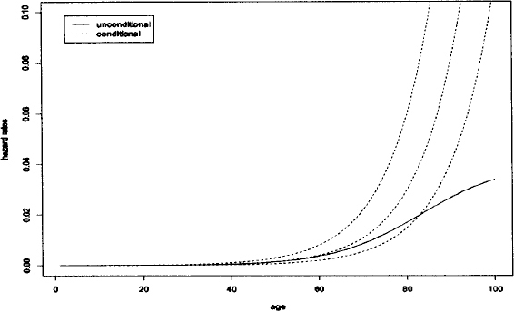
S(t|X,Z) characterizes the fraction of individuals surviving time t after beginning of the follow-up given the vector of observed covariates X and frailty Z. Note, that Equation 1 and Equation 2 describe the same model using different notions. Up to now, the model has been described at the conditional level (conditional on Z). However, this conditional model can not be observed. Consequently, for analysis it is necessary to consider the unconditional model. The survival function of the total population is the mean of the conditional survival functions (Equation 2). It can be viewed as the survival function of a randomly drawn individual. It is important to note that the conditional hazard function will usually not be similar to the observed unconditional hazard rate. What may be observed is the net result for individuals with different values of Z. The unconditional hazard rate may have a completely different shape than the conditional hazard rate, as shown in Figure 1.
Figure 1: Conditional and unconditional hazard rates in a simulated data set of human mortality. The dotted lines denote the conditional hazard rates for individuals with frailty 0.5, 1, and 2, respectively. The continuous line denotes the unconditional hazard rate
One natural problem in the application of frailty models is the choice of the frailty distribution. The frailty distributions most often applied are the gamma distribution [2], the positive stable distribution [10], the three-parameter distribution (PVF) [11], the compound Poisson distribution [12], and the log-normal distribution [13].
Univariate frailty models are popular. A few examples that can be consulted for more details are listed here. Aalen and Tretli [6] applied the compound Poisson distribution to testicular cancer data as discussed above. The idea of the model is that a subgroup of men are particularly susceptible to testicular cancer, which results in selection over time.
Another example is the analysis of malignant melanoma data including records of patients who had radical surgery for malignant melanoma (skin cancer) at the University Hospital of Odense in Denmark. Hougaard [14] compared the traditional Cox regression model with a gamma frailty and, PVF frailty model, respectively, based on these data.
Congdon [15] investigated the influence of different frailty distributions (gamma, inverse Gaussian, stable, binary) on total and cause-specific mortality from the London area (1988–1990).
Jeong et al. [16] applied the parametric gamma frailty model to a long-term follow-up trial in breast cancer to deal with converging hazards of the two treatment groups.
Henderson and Oman [17] focused on the quantification of the bias that occurs in estimated covariate effects and fitted marginal distributions when unobserved heterogeneity is present in the survival data, but this is ignored in a misspecified proportional hazards analysis.
A more detailed discussion of univariate frailty models including further examples can be found in Chapter 3 of the monograph by Wienke [18].
11.3 Multivariate Frailty Models
A second important application of frailty models is multivariate survival analysis. This kind of data occurs, for example, if lifetimes (or more general event times) of relatives (twins, couples, parent-child) or recurrent events such as infections of the same individual are considered. In such cases, independence between the clustered event times can often not be assumed. Multivariate models are able to account for the dependence between these event times. A commonly used and very general approach is to specify independence among observed data items conditional on a set of unobserved or latent variables [14]. The dependence structure in the multivariate survival model develops from a latent variable in the conditional models for multivariate survival times, for example, let S(t1|X1, Z) and S(t2|X2, Z) be the conditional survival functions of two related individuals with different vectors of observed covariates X1 and X2, respectively (see Equation 2).
Averaging over the distribution for the latent variables (e.g., using a log-normal, gamma, or positive stable distribution) then induces a multivariate model for the observed data. In the case of paired data, the survival function is of the form

where g denotes the density of frailty Z. In some situations (e.g., gamma frailty) this integral has an explicit analytical form, but this is not true in general (e.g. log-normal frailty).
Frailty models for multivariate survival data are derived under conditional independence assumption by specifying latent variables that act multiplicatively on the baseline hazard.
11.3.1 Shared Frailty Model
The shared frailty model is relevant to event times of related individuals, paired organs, and repeated measurements. The individuals in a cluster are assumed to share the same frailty Z, which is why this model is called the shared frailty model. It was introduced by Clayton [3] and studied in the monographs by Hougaard [14] and Duchateau and Janssen [19]. The survival times are assumed to be conditional independent with respect to the shared (common) frailty. For ease of presentation, the case of groups with pairs of individuals will be considered (bivariate failure times, for example, event times of twins or parent-child). Extensions to multivariate data are straightforward. Conditional on the frailty Z, the hazard function of an individual in a pair is of the form Zμ0(t) exp(β′X), where the value of Z is common to both event times in the pair, and thus is the cause for dependence between the survival times. Independence of the survival times within a pair corresponds to a degenerate frailty distribution [Z = 1, V (Z) = σ2 = 0]. In all other cases with σ2 > 0, the dependence is positive by construction of the model. Conditional on Z, the bivariate survival function is given as
![]()
In most applications, it is assumed that the frailty distribution is a gamma distribution with mean 1 and variance σ2. Averaging the conditional survival function produces survival functions of the form
Methods for sample size calculations in the shared frailty model can be found in Jahn-Eimermacher et al. [20].
Shared frailty explains correlation between subjects within clusters. However, it does have some limitations. First, it forces the unobserved factors to be the same within the cluster, which may not always reflect reality. For example, sometimes it may be inappropriate to assume that all partners in a cluster share all their unobserved risk factors. Second, the dependence between survival times within the cluster is based on marginal distributions of survival times. However, when covariates are present in a proportional hazards model with gamma distributed frailty, the dependence parameter and the population heterogeneity are confounded, which implies that the joint distribution can be identified from the marginal distributions [10]. Third, in most cases, shared frailty can only induce positive association within the cluster. However, some situations exist in which the survival times for subjects within the same cluster are negatively associated. For example, in the Stanford Heart Transplantation Study, generally the longer an individual must wait for an available heart, the shorter he or she is likely to survive after the transplantation. Therefore, the waiting time and the survival time afterwards may be negatively associated.
To avoid the above limitations of shared frailty models, correlated frailty models were developed.
11.3.2 Correlated Frailty Model
Originally, correlated frailty models were developed for the analysis of bivariate event time data, in which two associated random variables are used to characterize the frailty effect for each pair. For example, one random variable is assigned to partner 1 and one to partner 2 so that they would no longer be constrained to have a common frailty. These two variables are associated and have a joint distribution. Knowing one of them does not necessarily imply knowing the other. A restriction no longer exists on the type of correlation. These two variables can (especially in the correlated log-normal frailty model) also be negatively associated, which would induce a negative association between survival times. Assuming gamma distributed frailties, Yashin and Iachine [21] used the correlated gamma frailty model, resulting in a bivariate survival distribution of the form

More flexible regarding the correlation structure of the random effects is the log-normal correlated frailty model. This flexibility comes with the price that there exists no closed form of the unconditional likelihood function, which requires more sophisticated estimation procedures. A very general version of the model can be found in Vaida and Xu [22]. This approach underlines the important link of the log-normal frailty models to the well-developed generalized linear mixed models.
Examples of the use of correlated frailty models are various and emphasize the importance of this family of statistical models for survival data. A detailed presentation can be found in Chapter 5 of the monograph by Wienke [18].
11.4 Software
Stata 12 allows one to explore parametric as well as semiparametric gamma and inverse Gaussian frailty models. WinBugs is designed for analysis of frailty models with different frailty distribution, using Markov chain Monte Carlo methods. The R functions coxph, coxme, phmm and frailtypenal and the SAS macros SPGAM and SPLN3 are compared by simulations in Hirsch and Wienke [23] for shared gamma and log-normal frailty models. Since SAS 8.2 the shared log-normal frailty model is included in this software.
References
[1] M. Greenwood and G. Yule, An inquiry into the nature of frequency distributions representative of multiple happenings with particular reference to the occurrence of multiple attacks of disease or of repeated accidents. J. Roy. Stat. Soc. 1920; 83: 255–279.
[2] J. Vaupel, K. Manton, and E. Stallard, The impact of heterogeneity in individual frailty on the dynamics of mortality. Demography 1979; 16: 439–454.
[3] D. G. Clayton, A model for association in bivariate life tables and its application in epidemiological studies of familial tendency in chronic disease incidence. Biometrika 1978; 65: 141–151.
[4] D. Cox, Regression models and life-tables J. Roy. Stat. Soc. (B) 1972; 34: 187–220.
[5] K. Manton, E. Stallard, Methods for evaluating the heterogeneity of aging processes in human populations using vital statistics data: explaining the black-/white mortality crossover by a model of mortality selection. Human Biol. 1981; 53: 47–67.
[6] O. O. Aalen and S. Tretli, Analysing incidence of testis cancer by means of a frailty model. Cancer Causes Control 1999; 10: 285–292.
[7] P. K. Andersen, J. P. Klein, and M-J. Zhang, Testing for centre effects in multicentre survival studies: a Monte Carlo comparison of fixed and random effects tests. Stat. Med. 1999; 18: 1489–1500.
[8] C. Legrand, L. Duchateau, R. Sylvester, P. Janssen, J. van der Hage, C. van de Velde, and P. Therasse, Heterogeneity in disease free survival between centers: lessons learned from an EORTC breast cancer trial. Clin. Trials 2006; 3: 10–18.
[9] I. D. Ha, R. Sylvester, C. Legrand, and G. MacKenzie, Frailty modelling for survival data from multi-centre clinical trials. Stat. Med. 2011; 30: 2144–2159.
[10] P. Hougaard, A class of multivariate failure time distributions. Biometrika 1986; 73: 671–678.
[11] P. Hougaard, Survival models for heterogeneous populations derived from stable distributions. Biometrika 1986; 73: 387–396.
[12] O. O. Aalen, Heterogeneity in survival analysis. Stat. Med. 1988; 7: 1121–1137.
[13] C. A. McGilchrist and C. W. Aisbett, Regression with frailty in survival analysis. Biometrics 1991; 47: 461–466.
[14] P. Hougaard, Analysis of Multivariate Survival Data. New York: Springer, 2000.
[15] P. Congdon, Modeling frailty in area mortality. Stat. Med. 1995; 14: 1859–1874.
[16] J. Jeong, S. Jung, and S. Wieand, A parametric model for long-term follow-up data from phase III breast cancer clinical trials. Stat. Med. 2003; 22: 339–352.
[17] R. Henderson and P. Oman, Effect of frailty on marginal regression estimates in survival analysis. J. Roy. Stat. Soc. (B) 1999; 61: 367–379.
[18] A. Wienke, Frailty Models in Survival Analysis. Boca Raton, FL: Chapman & Hall/CRC, 2010.
[19] L. Duchateau, and P. Janssen, The Frailty Model. New York: Springer, 2008.
[20] A. Jahn-Eimermacher, K. Ingel, and A. Schneider, Sample size in cluster-randomized trials with time to event as the primary endpoint. Stat. Med. 2013; 32: 739–751.
[21] A. Yashin, J. Vaupel, and I. A. Iachine, Correlated individual frailty: an advantageous approach to survival analysis of bivariate data. Math. Pop. Studies 1995; 5: 145–159.
[22] F. Vaida, R. Xu, Proportional hazards model with random effects. Stat. Med. 2000; 19: 3309–3324.
[23] K. Hirschm, A. Wienke, Software for semi-parametric shared gamma and log-normal frailty models: An overview. Comput. Methods Programs Biomed. 2012; 107: 582–597.