
Chapter 27
Noncompartmental Analysis
27.1 Introduction
The objectives of noncompartmental analysis (NCA) are often assessing dose proportionality, showing bioequivalence, characterizing drug disposition, and obtaining initial estimates for pharmacokinetic models. Specific results and applications of NCA are as follows: (1) The area under the concentration-time curve (e.g. in plasma or serum) describes the extent of systemic drug exposure; the peak concentration and its timing indicate the rate of drug input (absorption), and (2) NCA provides estimates for clearance, volume of distribution, terminal half-life, mean residence time, and other quantities. Application 1 serves purely descriptive purposes and requires almost no assumptions. Importantly, application 2 does rely on several assumptions that are similar to the assumptions for compartmental modeling. Standard NCA requires frequent (blood) samples to estimate pharmacokinetic parameters reliably. Numerical integration is most commonly used for NCA after extravascular input. Fitting of disposition curves by a sum of exponential functions, for example, is the method of choice for intravenous bolus input.
NCA of an adequately designed clinical trial can provide robust estimates for extent of drug exposure and rate of absorption and other quantities. NCA estimates for clearance and volume of distribution rely on several assumptions that have to be critically considered for appropriate interpretation of NCA results.
NCA is a standard technique to determine the pharmacokinetics (PK) of a drug. After drug intake, the concentration-time profiles (e.g., in plasma or serum) are recorded and used to characterize the absorption, distribution, and elimination of the drug. Less frequently, concentrations in blood, saliva, or other body fluids, or amounts excreted unchanged in urine are used instead of or in addition to plasma or serum concentrations. NCA is the most commonly used method of PK data analysis for certain types of clinical studies like bioequivalence, dose linearity, and food effect trials.
The common feature of noncompartmental techniques is that no specific compartmental model structure is assumed. The most frequently applied method of NCA is slope height area moment analysis (SHAM analysis) [1,2].
For SHAM analysis, the area under the concentration-time curve (AUG) is most commonly determined by numerical integration or by curve fitting. Numerical integration is the noncompartmental method of choice for analysis of concentration-time data after extravascular input because absorption kinetics are often complex. In comparison to compartmental modeling, numerical integration has the advantage that it does not assume any specific drug input kinetics. For intravenous bolus data, fitting the concentration-time curves by a sum of exponentials is the noncompartmental method of choice.
This introductory article presents some standard applications of NCA of plasma (or serum) concentration data, as those applications are most commonly used. References for NCA of urinary excretion data and more advanced topics of NCA are provided. This article focuses on exogenous compounds and does not cover endogenous molecules. Our focus is (1) to describe studies and objectives for which NCA is well suited, (2) to provide and discuss assumptions of NCA, and (3) to present a practical guide for performing an NCA by numerical integration and basic approaches to choosing appropriate blood sampling times.
27.2 Terminology
27.2.1 Compartment
A compartment is a hypothetical volume that is used to describe the apparent homogeneous and well-mixed distribution of a chemical species. “Kinetically homogeneous” assumes that an instantaneous equilibration of a chemical compound (drug or metabolite) is found between all components of the compartment.
27.2.2 Parameter
A parameter is a primary constant of a quantitative model that is estimated from the observed data. For example, clearance (CL) and volume of distribution at steady state (Vss) are the two most important PK parameters.
27.2.3 Fixed Constant
Some models include fixed constants that are known (or assumed) a priori and are not estimated. Examples are stoichiometric coefficients or π.
27.2.4 Statistic
A statistic is a derived quantity that is computed from observed data or estimated model parameters.
Examples: The average plasma concentration is a statistic because it is computed from observed concentrations. Another statistic is the AUC. Under certain assumptions, the AUC is F. Dose/CL, with F being the fraction of drug that reaches the systemic circulation. The average clearance and its standard deviation are two statistics that can be calculated from individual clearance estimates of several subjects.
27.2.5 Comment
A one-compartment PK model can be defined by any two parameters, for example, by CL and Vss, by CL and t1/2, or by Vss and t/1/2. NCA estimates CL and t1/2 and derives Vss from other NCA statistics. However, physiologically, the parameterization by CL and Vss is more informative than the other two parameterizations because CL and Vss characterize the physiology of the body and the physicochemical properties of the drug. Half-life is determined by the primary PK parameters clearance and volume of distribution and should be called a statistic (or secondary parameter). For more complex PK models. Vss is calculated by residence time theory (see below and Reference 3).
27.3 Objectives and Features of Noncompartmental Analysis
Noncompartmental techniques can be applied to PK analyses of studies with a variety of objectives. Some of those objectives are:
- Bioavailability and bioequivalence studies,
- Food effect studies,
- PK interaction studies, and
- Dose proportionality studies.
NCA has appealing features, and the majority of studies in literature only report results from NCA. Some specific results from NCA and its features are:
However, it is important to be aware that NCA may be suboptimal or more difficult to apply in situations that need:
27.3.1 Advanced Noncompartmental Techniques
Various advanced noncompartmental techniques have been developed. A detailed presentation of these concepts is beyond the scope of this article. Some situations for which those advanced methods are superior to standard NCA are listed below.
Noncompartmental methods to analyze data with saturable elimination (Michaelis–Menten kinetics) have been developed by several authors [5–13]. Methods for the analysis of metabolite data [14–18], reversible metabolism [19–27], maternal-fetal disposition [28], enterohepatic recirculation [29], nonlinear protein binding [30] or capacity-limited tissue distribution [31], organ clearance models [19,32], and target-mediated drug disposition [33,34] and for modeling a link compartment [35] are available. Noncompartmental methods for sparse sampling [36–43] are often applied in preclinical PK and toxicokinetics. Veng-Pedersen presented [4,44] an overview of linear system analysis that is a powerful tool to determine absorption, distribution, and elimination characteristics and to predict concentrations for other dosage regimens.
Although these advanced methods have been developed, they are not as widely used as standard NCA, and some of these methods are not available in standard software packages.
27.4 Comparison of Noncompartmental and Compartmental Models
NCA is often called “model independent,” although this phrase is misleading and often misinterpreted [45–47]. The common feature of noncompartmental techniques is that they do not assume a specific compartmental model structure. NCA only can be described as (fully) model independent when it is exclusively used for descriptive purposes, for example, for recording the observed peak concentration (Cmax) and its associated time point (Tmax). Importantly, such a descriptive model-independent approach cannot be applied for extrapolation purposes.
The AUC from time zero to infinity (AUC0−∞) can be interpreted as a descriptive measure of systemic drug exposure (e.g., in plasma) for the studied dosage regimen. This interpretation requires the assumption of a monoexponential decline in concentrations during the terminal phase (or another extrapolation rule). However, the AUC is commonly used to calculate F, for example, in bioavailability and bioequivalence studies. As the AUC is determined by F. dose/clearance, the use of AUC to characterize F assumes that clearance is constant within the observed range of concentrations and over the time course of the data used to calculate the AUC. Therefore, all assumptions required for determination of clearance (see below) are implicitly made if AUC is used to characterize F.
Figure 1 compares the standard noncompartmental model and a compartmental model with two compartments. An important assumption of NCA is that drug is only eliminated from the sampling pool.
Figure 1: Comparison of the standard noncompartmental model and a compartmental model with two compartments

The two models shown in Figure 1 differ in the specification of the part of the model from which no observations were drawn (nonaccessible part of the system). In this example, the models differ only in the drug distribution part. For compartmental modeling, the user has to specify the complete model structure including all compartments, drug inputs, and elimination pathways. In Figure 1b, drug distribution is described by one peripheral compartment that is in equilibrium with the central compartment.
The “noncompartmental” model does not assume any specific structure of the nonaccessible part of the system. Any number of loops can describe the distribution, and each loop can contain any number of compartments. A more detailed list of the assumptions of standard NCA is provided below.
27.5 Assumptions of NCA and Its Reported Descriptive Statistics
NCA parameters like clearance and volume of distribution only can be interpreted as physiological or pharmacological properties of the body and the drug of interest if the assumptions of NCA are adequately met.
NCA relies on a series of assumptions Violating these assumptions will cause bias in some or all NCA results. This bias has been quantified and summarized by DiStefano and Landaw [45,46] for several examples.
Table 1 compares several key assumptions [36-50] between standard NCA and compartmental modeling. One key assumption of standard NCA is linear drug disposition (see Veng-Pedersen [44,50], Gillespie [47], and DiStefano and Landaw [46] for details). Although advanced methods to account for nonlinear drug disposition have been developed (see, e.g., Cheng and Jusko [8]), these techniques are seldom applied.
As shown in Table 1, the assumptions for a compartmental model with first-order disposition (“linear PK”) are similar to the assumptions of standard NCA. Compartmental models offer the flexibility of specifying various types of nonlinear disposition. This process is straightforward if a compartmental model is specified as a set of differential equations. Below is a discussion of the assumptions of NCA and compartmental modeling.
27.5.1 Assumption 1: Routes and Kinetics of Drug Absorption
Compartmental modeling uses a parametric function (e.g., first-order or zero-order kinetics) for drug absorption, whereas NCA does not assume a specific time course of drug input.
27.5.2 Assumptions 2 to 4: Drug Distribution
Standard NCA does not assume a specific model structure for the nonaccessible part of the system (“distribution compartments”). It only assumes that drug distribution is linear, for example, neither the rate nor the extent of distribution into the peripheral compartment(s) is saturable.
The user has to specify the complete structure and kinetics of drug transfer between all distribution compartments for compartmental modeling. Nonlinear drug disposition can be incorporated into compartmental models. Most compartment models assume linear distribution. In this case, the assumptions for drug distribution are similar for noncompartmental and compartmental methods.
Table 1: Comparison of Assumptions Between Standard NCA and Compartmental Modeling
| Standard NCA | Compartmental Modeling | |
| Absorptiona 1) Kinetics of drug absorption (drug input) |
no assumptions on rate of drug input required | has to be specified by the user, but can follow any time course |
| Distribution 2) Number and connectivity of peripheral compartments 3) Kinetics of drug transfer between sampling pool and peripheral compartment(s) 4) Extent of distribution into peripheral compartment(s) |
no assumptions assumed to be first-order (i.e. intercompartmental clearance assumed to be non-saturable)c assumed to be non-saturable, i.e. ‘protein’ binding in tissue is linear (non-saturable) |
must be specified explicitly usually similar to NCAb; other kinetics of drug transfer can be specified usually similar to NCAb; saturable extent of tissue distribution can be specified |
| Elimination 5) Routes of drug elimination 6) Kinetics of drug elimination |
elimination assumed to occur only from sampling pool first-order (non-saturable) elimination assumedc |
usually similar to NCAb; other routes can be specifiedd usually similar to NCAb; other kinetics of elimination can be specified |
| Other assumptions 7) Mono-exponential decline during terminal phase 8) Sampling time schedule 9) Time invariance of disposition parameters |
assumption required for calculation of terminal half-life and most NCA statistics an adequate representation of the whole plasma concentration time profile is requiredf Both methods assume that disposition parameters do not change within one occasion (e.g. during one dosing interval). |
assumption not required does not require samples to be drawn for the whole profile in each patiente |
aln the vast majority of cases both NCA and compartmental modeling assume that there is no absorption into any of the peripheral compartments. All drug molecules entering the system for the first time are assumed to enter into the sampling pool (central compartment). This assumption is more critical for endogenous compounds which might be synthesized at a peripheral site (see also DiStefano and Landaw (45,46).
bln most cases, the assumptions made for compartmental modeling are similar to the assumptions made for standard NCA (see Veng-Pedersen (44,50) and Gillespie (47) for details).
cThe concept of linear drug disposition is usually defined by the superposition principle (see Veng-Pedersen (44,50), Gillespie (47), and DiStefano and Landaw (46) for details).
dln order to retain identifiability of the model, the amount of drug loss from all but one of the elimination routes must be known or assumed (imputed).
eSampling time schedules can be optimized by selecting the most informative sampling times for a population PK model.
f Non-compartmental techniques for analysis of sparse data exist (36–43).
27.5.3 Assumption 5: Routes of Drug Elimination
Standard NCA assumes that all elimination occurs only from the sampling pool. Most compartmental models also assume that drug is eliminated only from the sampling (central) compartment (no elimination from any peripheral compartment). This assumption seems reasonable because the liver and the kidneys as the two main elimination organs are highly perfused organs and therefore in a rapid equilibrium with plasma (or serum), which is most commonly used for PK analysis. DiStefano and Landaw [45,46] discussed this assumption and the implications of its violation in detail.
Other routes of elimination can be specified for compartmental modeling. Nakashima and Benet [51] derived formulas for linear mammillary compartmental models with drug input into any compartment and drug elimination from any compartment.
27.5.4 Assumption 6: Kinetics of Drug Elimination
Standard NCA assumes that clearance is not saturable. As metabolism and renal tubular secretion are potentially saturable, the results of standard NCA for drugs with saturable elimination need to be interpreted cautiously. This cautious interpretation is especially important when plasma concentrations exceed the Michaelis-Menten constant of the respective saturable process. Several NCA methods that can account for saturable elimination are quoted above. However, those methods are not implemented in software packages like WinNonlinTM Pro or Thermo Kinetica, which makes them unavailable to most users.
Compartmental modeling offers great flexibility for specifying the elimination pathways and the kinetics of the elimination process (e.g., first-order, zero-order, mixed-order, target-mediated, etc.)
27.5.5 Assumptions 7 and 8: Sampling Times and Monoexponential Decline
For adequately chosen sampling times, the assumption that the last three (or more) observed concentrations characterize a monoexponential decline of concentrations during the terminal phase is often reasonable (see Weiss for details [52]). Standard NCA requires that the samples be collected during the whole concentration time profile. This time period is usually one dosing interval at steady state or at least three terminal half-lives after a single dose (see below for NCA of sparse data).
For studies with frequent sampling (12 or more samples per profile) at appropriately chosen time points, the AUC usually characterizes the total drug exposure well. For single-dose studies, it should be ensured that the AUC from time zero until the last observed concentration (AUC0−last) comprises at least 80% of AUC0−∞. Blood sampling times should be chosen so that at least two or more observations will be observed before the peak concentration in all subjects.
If the peak concentration is at the time of the first observation, then regulatory authorities like the Food and Drug Administration (FDA) [53,54] may require that a study be repeated because the safety of the respective formulation could not be established. In this situation, NCA cannot provide a valid measure for peak concentrations.
Blood sampling time schedules can be optimized to select the most informative sampling times for estimation of compartmental model parameters. The latter approach is more efficient as it requires (much) fewer blood samples per patient compared with NCA and is especially powerful for population PK analyses.
27.5.6 Assumption 9: Time Invariance of Disposition Parameters
This assumption is made very often for both NCA and compartmental modeling. The disposition parameters are assumed to be time-invariant (constant) within the shortest time interval required to estimate all PK parameters of interest. PK parameters may differ between two dosing intervals because two different sets of PK parameters can be estimated for each dosing interval by both NCA and compartmental methods. Caution is indicated for data analysis of drugs with inducible metabolism or when comedication may affect hepatic metabolism of the drug.
In summary, the assumptions of compartmental models with linear PK and of the standard NCA model are similar if NCA is used to derive PK parameters like CL, Vss, and F (as is most often done). The complete model structure and kinetics of all drug transfer processes must be defined for compartmental models, whereas NCA requires fewer assumptions on the model structure. Both standard compartmental models and the standard NCA model assume linear PK (see Veng-Pedersen [44,50], Gillespie [47], and DiStefano and Landaw [46] for more details). It is easier to specify nonlinear drug disposition for compartmental models than for NCA.
27.5.7 Assumptions of Subsequent Descriptive Statistics
NCA does not directly make any assumption about the distribution of NCA statistics between different subjects. However, most authors report the average and standard deviation for the distribution of NCA statistics and thereby assume that the average is an appropriate measure for the central tendency and that the standard deviation characterizes the variability adequately. The distribution of Tmax is especially problematic because it is determined primarily by the discrete distribution of the nominal sampling times.
It is often not possible to decide whether the between-subject variability follows a normal distribution, a log-normal distribution, or another distribution. Therefore, it is often helpful to report the median and representative percentiles (e.g., 5% to 95% percentile and 25% to 75% percentile) to describe the central tendency and variability of data by nonparametric statistics in addition to the average and standard deviation. If only data on a few subjects are available, then the 10% and 90% percentiles or the interquartile range are usually more appropriate than the 5% and 95% percentiles. Reporting only the median and range of the data does not provide an accurate measure for dispersion, especially for studies with a small sample size.
27.6 Calculation Formulas for NCA
This section presents numerical integration methods to determine the AUC that is most commonly used to analyze plasma (or serum) concentrations after extravascular dosing. Additionally, fitting of concentration-time curves by a sum of exponential functions is described. The latter is the noncompartmental method of choice for intravenous bolus input. The concentration time curves after intravenous bolus input are called disposition curves because drug disposition comprises drug distribution and elimination but not the absorption process. Both methods are noncompartmental techniques because they do not assume a specific model structure. It is important to note that several compartmental models will result in biexponential concentration time profiles.
It is appealing that the numerical integration of a standard NCA can be performed with a hand calculator or any spreadsheet program. Nonlinear regression to describe disposition curves can be done by standard software packages like ADAPT, WinNonlinTM Pro, Thermo Kinetica, SAAM II, EXCEL, and many others. Performing an NCA with a hand calculator or self-written spreadsheets is good for learning purposes. However, the use of validated PK software for NCA of clinical trials is vital for projects to be submitted to regulatory authorities. Audit trail functionality is an important advantage of validated PK software packages.
27.6.1 NCA of Plasma or Serum Concentrations by Numerical Integration
Numerical integration is the most commonly used method to determine the AUC and other moments of the plasma (or serum) concentration-time curve after extravascular input. This method is also often applied for infusion input if the duration of infusion is nonnegligible. Numerical integration requires a function neither to describe the whole concentration-time curve nor to describe the rate of drug absorption (e.g., first-order or zero-order input).
The Cmax and Tmax are directly recorded from the observed concentration-time data. NCA assumes that the concentration during the terminal phase declines monoexponentially. Subsequently, linear regression on a semilogarithmic scale is used to determine the slope (− λz) of the concentration-time curve during the terminal phase. Terminal half-life is calculated as
![]()
A guide for the most appropriate selection of observations for estimation of terminal half-life is described below. Figure 2 illustrates the calculation of terminal half-life for one subject. In this example, the last five observations were used to estimate the terminal slope.
Figure 2: Determination of terminal half-life after a single oral dose

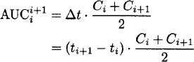
The area under the plasma concentration-time curve is most often determined by the trapezoidal method. The plasma concentration-time profile is usually linearly (or logarithmically) interpolated between two observations. The formulas apply to linear and logarithmic interpolation, and Ci denotes the ith observed concentration:
Linear interpolation:
Logarithmic interpolation:
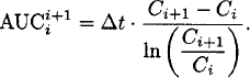
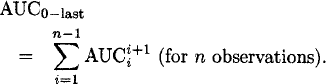
Figure 3 shows the calculation of trapezoids for data after a single oral dose by the linear interpolation rule. The sum of the individual trapezoids yields the AUC from time zero to the last quantifiable concentration:
Figure 3: Calculation of the AUC by the linear trapezoidal rule

Linear interpolation is usually applied if concentrations are increasing or constant (Ci+1 ≥ Ci), and logarithmic interpolation is often used if concentrations are decreasing (Ci+1 < Ci). Note that the log-trapezoidal rule is invalid when Ci+1 = Ci and when Ci is zero.
Plasma concentration-time profiles are curved to the right during an intravenous infusion at a constant rate (see Figure 4) and also tend to be curved to the right for extravascular administration. Therefore, linear interpolation to calculate the AUC is a reasonable approximation if Ci+1 ≥ Ci.
Figure 4: Interpolation between plasma concentration-time points by the linear and logarithmic trapezoidal methods for a 2-h infusion (sampling times: 0, 0.5, 2, 2.5, 4, and 6h)

After the end of infusion, drug concentrations often decline mono-, bi-, or tri-exponentially (see Figure 4). The number of exponential phases can be assessed visually when drug concentrations are plotted on a log scale versus time. Therefore, assuming an exponential decline (equivalent to a straight line on log scale) is often a good approximation for the AUC calculation if Ci+1 < Ci.
Figure 4 shows that linear interpolation approximates the true plasma concentration-time curve slightly better than the logarithmic interpolation during the infusion. After the end of infusion, logarithmic interpolation approximates the true curve better then linear interpolation—as expected.
The difference between linear and logarithmic interpolation tends to be small if blood samples are frequently drawn. Differences are expected to be larger for less-frequent blood sampling. Linear and logarithmic interpolation have been compared with interpolation by higher-order polynomials and splines [55,56]. For PK data, the linear trapezoidal rule for increasing or constant concentrations and the log-trapezoidal rule for decreasing concentrations is usually a good choice [19] because those methods are stable and reasonably accurate even for sparse data. Although higher-order polynomials and spline functions perform better for some data sets, these methods are potentially more sensitive to error in the data and are not available in most standard software packages.
The AUC from the last concentration (Clast) to time infinity (AUClast−∞) is extrapolated assuming a log-linear decline of concentrations during the terminal phase: AUClast−∞ = ![]() .
.
Standard software packages like WinNonlinTM Pro, Thermo Kinetica, and others provide two options for specifying Clast: One can use the last observed concentration as Clast. Alternatively, the concentration predicted by log linear regression at the time of the last observation may be used as Clast to estimate λz. The current FDA guideline for bioavailability and bioequivalence studies [53] recommends that the last “measured” (observed) concentration should be used. The FDA guideline does not provide a reason why this method is proposed. Theoretically, the last predicted concentration will be more precise than an observed value if the assumptions for estimation of the terminal half-life are met. Use of the last observed concentration may yield a large bias if this concentration was an “outlier” with a high value, because it would cause a longer half-life and therefore would affect both terms in the equation for AUClast−∞.
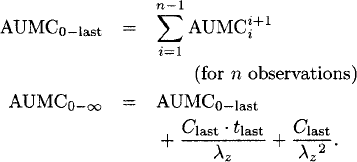
The AUC from time zero to infinity (AUC0−∞) is calculated as
![]()
The residual area is calculated as 1 − AUC0−last / AUC0−∞. Residual areas above 20% are considered too large for reliable estimation of AUC0−∞ and therefore also for CL. The uncertainty in the calculated area under the first moment concentration-time curve from time zero to infinity (AUMC0−∞) is even larger compared with the uncertainty in AUC0−∞ for larger residual areas.
The (apparent) total clearance (CL/F) is calculated from the administered dose and AUC0−∞ as
![]()
For intravenous administration, the extent of drug reaching the systemic circulation (F) is 100% by definition, and the ratio of dose and AUC0−∞ yields total clearance (CL). As F is mathematically not identifiable after extravascular administration without an intravenous reference dose, only CL/F can be derived after extravascular administration.
The volume of distribution during the terminal phase (Vz) can be calculated from CL and λz. As shown by several authors [57,58], Vz is not an independent parameter that characterizes drug disposition because it depends on, for example, the estimate for clearance. Volume of distribution at steady state (Vss) is a better measure for volume of distribution than Vz. The estimate for clearance does not affect the estimate of Vss if drug is only eliminated from the sampling pool. Vss can always be calculated from data that allow one to calculate Vz (see below).
Gobburu and Holford [58] pointed out that the finding of an altered Vz, for example, in a special patient population, may lead to the inappropriate conclusion of changing the loading dose in this patient population. Because of the potential misuse of Vz, the use of Vz should be discouraged [58].
Statistical moment theory [59] is used to calculate the mean residence time (MRT). The MRT is calculated from AUMC0−∞ and AUC0−∞. The AUMC is calculated as
Linear interpolation:
![]()
Logarithmic interpolation:
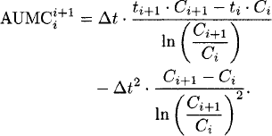
The AUMC from time zero to the last observed concentration (AUMC0−last) and from time zero to infinity (AUMC0−∞) are calculated as
For steady-state data (dosing interval: τ), the AUMC0−∞ can be calculated as [60]
![]()
The mean residence time (MRT) is calculated as
![]()
[The AUMC0−last and AUC0−last should not be used for calculation of MRT, because such a calculation yields systematically biased (low) estimates for the MRT.]
For an intravenous bolus administration, the MRT is equal to the mean disposition residence time (MDRT). The MDRT is the average time a drug molecule stays in the systemic circulation [44]. The MDRT is often called MRTiv (iv indicates iv bolus input). We prefer to write MDRT to refer specifically to drug disposition.
If peripheral venous blood is sampled, then the mean transit time of drug molecules from arterial blood to the sampling site needs to be considered for calculation of MDRT, at least for drugs with a short MDRT (see Weiss [3,61] and Chiou [62] for details).
Vss is calculated as
![]()
For high-clearance drugs, calculation of Vss is more complex [3,19,32,63].
The MDRT determines the accumulation ratio (RA), which is defined as the average amount of drug in the body at steady state (after multiple administration) divided by the bioavailable maintenance dose (F . MD). The RA is MDRT divided by the dosing interval [3]. Furthermore, MDRT determines the accumulation time and the washout time as described by Weiss [64,65].
For noninstantaneous drug input (e.g., extravascular dose or constant-rate infusion), the ratio of AUMC0−∞ and AUC0−∞ yields the mean total residence time (MTRT), which is the sum of the mean input time (MIT) and MDRT.
For constant-rate (intravenous) infusion with a given duration of infusion (Tinf), the MIT equals Tinf/2. Therefore, the MDRT can be calculated as
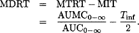
The MIT after extravascular administration is more difficult to calculate without an intravenous reference. The MIT can be determined as the difference of MTRT and MDRT, when both an extravascular and intravenous dose are given to the same subject on different occasions.
To calculate Vss after extravascular administration, the MIT needs to be subtracted from the MTRT [66,67]. The MIT can be approximated by Tmax/2 if the input process is close to zero-order [common for drugs in class I of the biopharmaceutical classification system (BCS) because of a zero-order release of drug from stomach; BCS class I drugs have high solubility and high permeability]. If the process seems to be first-order, then MIT can be approximated by Tmax/(3 · ln(2)) because Tmax commonly occurs at around three times the first-order absorption half-life.
The extent of bioavailability (F) is typically determined by giving a single oral dose and a single intravenous dose on two different occasions (with an appropriate washout period) to the same subject. From these data, CL, Vss, MDRT, MIT, and F can be calculated by the formulas shown above. The ratio of the AUG after oral and intravenous dosing characterizes F:
![]()
The MIT values for each subject can be calculated as the difference of MTRT and MDRT. Assuming a first-order absorption (without lag time), MIT is the inverse of the first-order absorption rate constant (1/ka). The MIT can be correlated with the mean dissolution time determined in vitro to establish an in vitro/in vivo correlation, for example, to compare the release characteristics of various modified release formulations [68,69].
27.6.2 NCA. of Plasma or Serum Concentrations by Curve Fitting
For NCA of concentration time curves after intravenous bolus administration, the results from numerical integration are very sensitive to the timing of samples and to errors in the data (e.g., measurement error or undocumented deviations in the sampling time). For such data, use of analytical functions to fit the disposition curves is the method of choice. For monotonously decreasing concentrations, a sum of exponential functions is often a good choice to describe disposition curves. No a priori reason exists for choosing a sum of exponential functions. Some authors have used other functions like gamma curves [52,70–72].
Most commonly, disposition curves [concentration CD(t at time t] are described by a sum of n exponential functions:
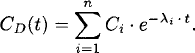
The Ci is the intercept of each exponential phase, and −λi is the associated slope on semilogarithmic scale. The kth moment (MOCk) of the disposition curve can be calculated as [3]
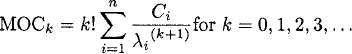
As AUC is the area under the zerothmoment concentration-time curve and AUMC is the area under the first-moment concentration time-curve, this formula yields:

Figure 5 shows an example of a tri-exponential disposition curve. The following parameter values were used for simulation: C1 = 50 mg/L, C2 = 40 mg/L, C3 = 10 mg/L, λ1 = 2.77 h−1, λ2 = 0.347 h−1, and λ3 = 0.0578 h−1. The disposition curve shows three different slopes on a semilogarithmic plot versus time. The contribution of the individual exponential functions is indicated. Fitting the concentration-time profiles by a sum of exponential functions may be helpful to interpolate between observed concentrations. This sum of exponentials could be used, for example, as forcing function for a pharmacodynamic model.
Figure 5: Disposition curve after iv bolus administration with three exponential functions

The parameters of this sum of exponential functions can be estimated by software packages like ADAPT, WinNonlinTM Pro, Thermo Kinetica, SAAM II, and many others. Use of an appropriate error variance model (or of an adequate weighting scheme) is highly recommended. A thorough discussion of nonlinear regression is beyond the scope of this article. See Gabrielsson and Weiner [73] and the manuals of the respective software packages for details.
27.6.3 NCA with Plasma or Serum Concentrations and Amounts in Urine
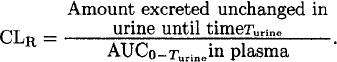
Urinary excretion rates can be used instead of plasma concentrations to characterize the PK profile of drugs excreted (primarily) by the kidneys. The majority of studies use plasma (or serum) concentrations to determine the PK. If the excretion of drug into urine is studied in addition to plasma concentrations, then renal clearance (CLR) and nonrenal clearance/F can be calculated in addition to total clearance. The total amount excreted unchanged in urine from time zero up to the last collected urine sample (Turine) and the AUC from time zero to Turine are used to calculate CLR:
Importantly, this formula yields renal clearance (and not renal clearance/F) both for intravenous and for extravascular administration because the amount recovered in urine is known. Nonrenal clearance (CLNR) is calculated as the difference between total (CL) and renal clearance (CLR) for intravenous administration. Apparent nonrenal clearance is calculated as the difference between CL/F and CLR for extravascular administration. If F is less than 100%, then this difference will not be equal to CLNR after intravenous administration divided by F because the estimate for CLR does not include F.
In addition to clearance, MDRT and therefore volume of distribution at steady state can be calculated from urinary excretion data as described by Weiss [3].
The urinary excretion rate is calculated as amount of drug excreted unchanged in urine per unit of time. A urinary excretion rate versus time plot is one method to estimate terminal elimination half-life based on urine data [see Rowland and Tozer [74] for details]. The calculated half-life from urinary excretion data should be similar to the half-life calculated from plasma data.
27.6.4 Superposition Methods and Deconvolution
Superposition methods assume that the concentration-time profiles of each dose can be added if two doses are given at the same or at different times because the concentrations achieved by each dose do not influence each other [47]. A linear pharmacokinetic system has this property. This situation allows one to simulate plasma concentration-time profiles after multiple doses by adding up concentration time profiles after various single doses at the respective dosing times. Such a nonparametric superposition module is implemented, for example, in WinNonlinTM Pro, and a similar module (on convolution) is available in Thermo Kinetica.
In pharmacokinetics, deconvolution is often used to determine the in vivo release profile, for example, of a modified release formulation. The disposition curve after intravenous bolus administration (impulse response of the system) can be used in combination with the plasma concentration time curve of an extravascular formulation to determine the in vivo release profile. The Wagner–Nelson method [75–78] that is based on a one-compartment model and the Loo–Riegelman method that can account for multiple disposition compartments [79,80] have been applied extensively. These methods subsequently were greatly extended [44,50,73, 81–83]. A detailed description of those algorithms is beyond the scope of this article. Convolution/deconvolution methods are available in WinNonlinTM Pro and in Thermo Kinetica.
27.7 Guidelines for Performance of NCA Based on Numerical Integration
Before running any PK analysis, it is very-helpful to prepare various plots of the observed concentration-time data. Typically, the observed individual concentration-time data are plotted on linear and semilogarithmic scales (i.e., concentrations on log-scale vs. time on linear scale). A log2 scale is often a good choice to visualize concentration versus time data because half-life can be visualized more easily by such a plot.
These plots usually are prepared for all subjects at the same time (“spaghetti plots”) and for each subject individually. An intraindividual comparison of the observed data for different treatments is often helpful. If different doses were given to the same subject, then plotting dose-normalized concentrations is helpful to assess dose linearity visually according to the superposition principle. Calculation of descriptive statistics in addition to the individual observed data provides useful summary statistics. The average ± standard deviation and the median (25%–75% percentiles) or other representative percentiles are often plotted versus time for each treatment. These observed data plots might already reveal that some assumptions like first-order elimination might not be appropriate.
Actual, instead of nominal, protocol sampling times should always be recorded and used for PK analysis. For the very common case that numerical integration by the trapezoidal rule is applied, the two most important user decisions are (1) determination of the terminal phase and (2) choice of the integration rule for the AUC. The choice of the most appropriate AUC calculation method is discussed above. Some guidelines for determining the terminal phase are shown below.
27.7.1 How to Select Concentration Data Points for Estimation of Terminal Half-Life
The following rules provide some practical guidelines for determination of the terminal phase of the concentration-time profile:
Other criteria for the number of data points may also be appropriate. Proost [84] compared various criteria to estimate λz by simulating profiles for a one-compartment model and concluded that various criteria (including the r2 and r2-adjusted criteria) had comparable bias and precision for the estimate of λz.
Irrespective of the criterion chosen, it seems reasonable to ensure an appropriate selection of data points to estimate the terminal half-life by visual inspection of the observations and the predicted regression line in each subject.
Probably no set of guidelines is applicable to all data sets. This set of rules may need to be revised, if the precision of the bioanalytical assay is low at low concentrations. Terminal half-life sometimes cannot be well determined by NCA for extended-release formulations or for data after multiple dosing, especially if the dosing interval is shorter than about twice the terminal half-life. It may be very helpful to report the median instead of the arithmetic mean to describe the central tendency of terminal half-life if NCA indicates extremely long half-lives for some subjects. Compartmental modeling may be more powerful in these situations [85].
The concentrations during the terminal phase used in linear regression on semilogarithmic scale often span a wide range (sometimes more than a factor of 100 between the highest and lowest concentration). This consideration is important for choosing an adequate weighting scheme. Importantly, unweighted linear regression (uniform weighting) on semilogarithmic scale is approximately equal to assuming a constant coefficient of variation error model. Therefore, unweighted linear regression on semilogarithmic scale is usually an adequate weighting scheme for NCA.
27.7.2 How to Handle Samples Below the Quantification Limit
The best way to handle observations reported as being below the limit of quantitation is to ask the chemical analyst to supply the measured values. It may be necessary to tell and convince the analytical team that reporting the measured concentration value for samples “below the quantification limit” (BQL) contributes valuable information. These low concentrations can be adequately weighted when compartmental modeling techniques are applied. No good PK or regulatory reason exists not to use these observations. However, very good statistical theory supports the idea that discarding these values will bias the results of subsequent PK analysis (86–94).
Concentrations at the first time points for extravascular administration and during the terminal phase are often reported to be BQL by the analytical laboratory.
A thorough discussion of handling BQL samples in a PK data analysis is beyond the scope of this article. Population PK modeling offers more powerful methods for dealing with BQL samples. As a practical guide for NCA, the following procedure can be applied if the only available information is that the respective samples were reported to be BQL:
An unreasonable option is to ignore the BQL samples before the first quantifiable concentration and to calculate the first trapezoid from time zero to the first quantifiable concentration, because this calculation would yield a much larger overestimation of the AUC compared with the small underestimation described above.
Figure 6: Example of a plasma concentration time profile with various samples reported to be below the quantification limit (BQL) that is reported to be 1 mg/L

If the terminal phase is adequately described by the last quantifiable concentrations and if the residual area is below 5%, then ignoring all BQL samples after the last quantifiable concentration seems to be most reasonable. Imputing the first BQL sample at 6 h (see Figure 6) to be half of the quantification limit (or any other pre-specified value) is likely to yield (slightly) biased estimates for terminal half-life in an NCA. Importantly, such an imputed sample should not be used for calculation of residual area.
27.7.3 NCA for Sparse Concentration-Time Data
NCA methods for sparse concentration-time data have been developed [36–43]. These methods are often applied for preclinical PK, toxicokinetic, and animal studies for which usually only sparse data are available.
Bailer [36] originally proposed a method that uses concentration-time data from destructive sampling (one observation per animal) to estimate the average AUC up to the last observation time and to derive the standard error of the average AUC. Assume, for example, that 20 animals are sacrificed at 5 different time points (4 animals at each time point). The average and variance of the concentration at each time point are calculated, and the linear trapezoidal rule is used to derive the average AUC. Bailer provided a formula for the standard error of the average AUC. If various treatments are compared, then the average AUC can be compared statistically between different treatments by use of this standard error. Extensions to the Bailer method were developed (41–43) and were recently implemented into version 5 of WinNonlinTM Pro. Sparse sampling methods for NCA will also become available in the next version of Thermo Kinetica.
Subsequently, bootstrap resampling techniques for sparse data (one observation per animal) were developed and evaluated [37–39]. The so-called pseudoprofile-based bootstrap [38] creates pseudoprofiles by randomly sampling one concentration from, for example, the four animals at each time point. One concentration is drawn at each of the five time points. These five concentrations represent one pseudoprofile. Many pseudoprofiles are randomly generated, and an NCA is performed for each pseudoprofile. Summary statistics are computed to calculate the between-subject variability and standard error of the NCA statistics of interest (see Mager and Goller [38] for details).
27.7.4 Reporting the Results of an NCA
The PK parameters and statistics to be reported for an NCA depend on the objectives of the analysis and on the types of data. Regulatory guidelines list several PK parameters and statistics to be reported from an NCA [53,54]. A detailed report on the design, analysis, and reporting of clinical trials by NCA has been published by the Association for Applied Human Pharmacology (AGAH) [54]. Valuable guidelines can also be found on pages 21 to 23 of the FDA guidelines for bioavailability and bioequivalence studies [53].
It is often helpful for subsequent analyses to report the average ± SD (or geometric mean and %CV) and median (percentiles) of the following five NCA statistics: AUG, Cmax, Tmax, t1/2, and AUMC. Reporting the results on CL and Vss provides insight into the drug disposition.
If the average and SD of these five NCA statistics are reported, then the so-called back analysis method [95] can be applied to convert NCA statistics into compartmental model parameters. Alternatively, the individual NCA statistics in each subject can be used instead of average and SD data. One has to decide based on literature data, for example, before applying the back analysis method, if a one- or two-compartment model is likely to be more appropriate for the drug of interest. The back analysis method provides estimates for the mean and variance of the model parameters for a one- or two-compartment model. The resulting PK parameter estimates can be used, for example, to build a population PK model and to run clinical trial simulations. The back analysis method allows one to run such simulations based on NCA results without the individual concentration time data. However, if individual concentration-time data are available, population PK analysis is the preferred method of building a population PK model.
27.7.5 How to Design a Clinical Trial That Is to Be Analyzed by NCA
It is possible to optimize the design of clinical trials (e.g., of bioequivalence studies) that are to be analyzed by NCA. However, those methods rely on compartment models in a population PK analysis and clinical trial simulation and are not covered in this article. Some practical guidelines for selection of appropriate sampling time points are provided below. This article focuses on NCA analysis by numerical integration for the most common case of extravascular dosing. The methods presented here are not as powerful as optimization of the study design by clinical trial simulation but may provide a basic guide.
Before planning the sampling time schedule, one needs at least some information on the blood volume required for drug analysis and on the sensitivity of the bioanalytical assay. Some knowledge on the expected average concentration-time profile of the drug is also assumed. The FDA [53] recommends 12 to 18 blood samples (including the predose sample) to be taken per subject and per dose. Cawello [96] and the AGAH working group recommend in total 15 blood samples to be drawn. Five samples (including the predose sample) should be drawn before Tmax. Another five samples are to be drawn between Tmax and one half-life after Tmax, and another five samples should be drawn up to five half-lives after Tmax.
If one assumes that the median Tmax is at 1.5 h and that the average terminal half-life is 5 h, then this recommendation would yield, for example, the following sampling times: 0 h (predose), 0.33, 0.67, 1.00, 1.50, 2.00, 2.50, 3.00, 4.00, 6.00, 8.00, 12.0, 16.0, 24.0, and 32.0 h post dose.
Cawello [96] recommends that each of the three intervals described above should contain four samples if only 12 samples can be drawn in total. This recommendation would yield, for example, the following sampling times: 0 h (predose), 0.50, 1.00, 1.50, 2.00, 3.00, 4.00, 6.00, 10.0, 16.0, 24.0, and 32.0 h post dose.
Such a sampling schedule may need to be modified, for example, for drugs with a large variability in terminal half-life or in Tmax. If the variability in Tmax is large, then more frequent sampling may be required during the first hour post dose in this example. Overall, this sampling schedule should provide low residual areas and a robust estimate for the terminal half-life.
27.8 Conclusions and Perspectives
NCA is an important component of the toolbox for PK analyses. It is most applicable for studies with frequent sampling. Numerical integration, for example, by the trapezoidal rule, is most commonly used to analyze data after extravascular dosing. Fitting of disposition curves by a sum of exponential functions is the non-compartmental method of choice for analysis of concentrations after intravenous bolus dosing. Noncompartmental methods for handling sparse data have been developed and are available in standard software packages. Standard NCA is straightforward and can be conveniently applied also by nonprofessional users.
It is important to recognize the assumptions and limitations of standard NCA. Almost all applications of NCA require a series of assumptions that are similar to the assumptions required for compartmental modeling. Violation of the assumptions for NCA will result in biased parameter estimates for some or all PK parameters.
From a regulatory perspective, NCA is appealing as it involves minimal decision making by the drug sponsor or drug regulator.
NCA can provide robust estimates of many PK parameters for studies with frequent sampling. For these studies, NCA and compartmental modeling often complement each other, and NCA results may be very helpful for compartmental model building. Therefore, NCA may be very valuable for PK data analysis of studies with frequent sampling, irrespective of whether the study objectives require subsequent analysis by compartmental modeling.
Acknowledgments. We thank one of the reviewers and Dr. William J. Jusko for comments on this manuscript. Jürgen Bulitta was supported by a postdoctoral fellowship from Johnson & Johnson.
References
[1] O. Caprani, E. Sveinsdottir, and N. Lassen, SHAM, a method for biexponential curve resolution using initial slope, height, area and moment of the experimental decay type curve. J. Theor. Biol. 1975; 52: 299–315.
[2] N. Lassen and W. Perl, Tracer Kinetic Methods in Medical Physiology. New York: Raven Press, 1979.
[3] M. Weiss, The relevance of residence time theory to pharmacokinetics. Eur. J. Clin. Pharmacol. 1992; 43: 571–579.
[4] P. Veng-Pedersen, Noncompartmentally-based pharmacokinetic modeling. Adv. Drug Deliv. Rev. 2001; 48: 265–300.
[5] P. Veng-Pedersen, H. Y. Cheng, and W. J. Jusko, Regarding dose- independent pharmacokinetic parameters in nonlinear pharmacokinetics. J. Pharm. Sci. 1991; 80: 608–612.
[6] A. T. Chow and W. J. Jusko, Application of moment analysis to nonlinear drug disposition described by the Michaelis-Menten equation. Pharm. Res. 1987; 4: 59–61.
[7] H. Y. Cheng and W. J. Jusko, Mean residence time of drugs in pharmacokinetic systems with linear distribution, linear or nonlinear elimination, and noninstantaneous input. J. Pharm. Sci. 1991; 80: 1005–1006.
[8] H. Y. Cheng and W. J. Jusko, Mean residence time concepts for pharmacokinetic systems with nonlinear drug elimination described by the Michaelis-Menten equation. Pharm. Res. 1988; 5: 156–164.
[9] H. Cheng, W. R. Gillespie, and W. J. Jusko, Mean residence time concepts for non-linear pharmacokinetic systems. Biopharm. Drug Dispos. 1994; 15: 627–641.
[10] H. Cheng, Y. Gong, and W. J. Jusko, A computer program for calculating distribution parameters for drugs behaving nonlinearly that is based on disposition decomposition analysis. J. Pharm. Sci. 1994; 83: 110–112.
[11] P. Veng-Pedersen, J. A. Widness, L. M. Pereira, C. Peters, R. L. Schmidt, and L. S. Lowe, Kinetic evaluation of nonlinear drug elimination by a disposition decomposition analysis. Application to the analysis of the nonlinear elimination kinetics of erythropoietin in adult humans. J. Pharm. Sci. 1995; 84: 760–767.
[12] M. Weiss, Mean residence time in nonlinear systems? Biopharm. Drug Dispos. 1988; 9: 411–412.
[13] D. J. Cutler, A comment regarding mean residence times in non-linear systems. Biopharm. Drug Dispos. 1989; 10: 529–530.
[14] H. Y. Cheng and W. J. Jusko, An area function method for calculating the apparent elimination rate constant of a metabolite. J. Pharmacokinet. Biopharm. 1989; 17: 125–130.
[15] A. T. Chow and W. J. Jusko, Michaelis-Menten metabolite formation kinetics: equations relating area under the curve and metabolite recovery to the administered dose. J. Pharm. Sci. 1990; 79: 902–906.
[16] M. Weiss, Use of metabolite AUC data in bioavailability studies to discriminate between absorption and first-pass extraction. Clin. Pharmacokinet. 1990; 18: 419–422.
[17] M. Weiss, A general model of metabolite kinetics following intravenous and oral administration of the parent drug. Biopharm. Drug Dispos. 1988; 9: 159–176.
[18] J. B. Houston, Drug metabolite kinetics. Pharmacol Ther. 1981; 15: 521–552.
[19] W. J. Jusko, Guidelines for collection and analysis of pharmacokinetic data. In: M. E. Burton, L. M. Shaw, J. J. Schentag, and W. E. Evans (eds.), Applied Pharmacokinetics & Pharmacodynamics, 4th ed. Philadelphia, PA: Lippincott Williams and Wilkins, 2005.
[20] H. Y. Cheng and W. J. Jusko, Mean residence times and distribution volumes for drugs undergoing linear reversible metabolism and tissue distribution and linear or nonlinear elimination from the central compartments. Pharm. Res. 1991; 8: 508–511.
[21] H. Y. Cheng and W. J. Jusko, Mean residence time of drugs showing simultaneous first-order and Michaelis-Menten elimination kinetics. Pharm. Res. 1989; 6: 258–261.
[22] H. Y. Cheng and W. J. Jusko, Mean interconversion times and distribution rate parameters for drugs undergoing reversible metabolism. Pharm. Res. 1990; 7: 1003–1010.
[23] H. Y. Cheng and W. J. Jusko, Mean residence times of multicompartmental drugs undergoing reversible metabolism. Pharm. Res. 1990; 7: 103–107.
[24] H. Y. Cheng and W. J. Jusko, Mean residence time of oral drugs undergoing first-pass and linear reversible metabolism. Pharm. Res. 1993; 10: 8–13.
[25] H. Y. Cheng and W. J. Jusko, Pharmacokinetics of reversible metabolic systems. Biopharm. Drug Dispos. 1993; 14: 721–766.
[26] S. Hwang, K. C. Kwan, and K. S. Albert, A linear mode of reversible metabolism and its application to bioavailability assessment. J, Pharmacokinet. Biopharm. 1981; 9: 693–709.
[27] W. F. Ebling, S. J. Szefler, and W. J. Jusko, Methylprednisolone disposition in rabbits. Analysis, prodrug conversion, reversible metabolism, and comparison with man. Drug Metab. Dispos. 1985; 13: 296–304.
[28] M. N. Samtani, M. Schwab, P. W. Nathanielsz, and W. J. Jusko, Area/-moment and compartmental modeling of pharmacokinetics during pregnancy: applications to maternal/fetal exposures to corticosteroids in sheep and rats. Pharm. Res. 2004; 21: 2279–2292.
[29] M. S. Roberts, B. M. Magnusson, F. J. Burczynski, and M. Weiss, Enterohepatic circulation: physiological, pharmacokinetic and clinical implications. Clin. Pharmacokinet. 2002; 41: 751–790.
[30] H. Cheng and W. R. Gillespie, Volumes of distribution and mean residence time of drugs with linear tissue distribution and binding and nonlinear protein binding. J. Pharmacokinet. Biopharm. 1996; 24: 389–402.
[31] F. M. Gengo, J. J. Schentag, and W. J. Jusko, Pharmacokinetics of capacity-limited tissue distribution of methicillin in rabbits. J. Pharm. Sci. 1984; 73: 867–873.
[32] R. Nagashima, G. Levy, and R. A. O’Reilly, Comparative pharmacokinetics of coumarin anticoagulants. IV. Application of a three-compartmental model to the analysis of the dose-dependent kinetics of bishydroxycoumarin elimination. J. Pharm. Sci. 1968; 57: 1888–1895.
[33] D. E. Mager, Target-mediated drug disposition and dynamics. Biochem. Pharmacol. 2006; 72: 1–10.
[34] D. E. Mager and W. J. Jusko, General pharmacokinetic model for drugs exhibiting target-mediated drug disposition. J. Pharmacokinet. Pharmacodyn. 2001; 28: 507–532.
[35] H. Cheng and W. J. Jusko, Disposition decomposition analysis for pharmacodynamic modeling of the link compartment. Biopharm. Drug Dispos. 1996; 17: 117–124.
[36] A. J. Bailer, Testing for the equality of area under the curves when using destructive measurement techniques. J. Pharmacokinet. Biopharm. 1988; 16: 303–309.
[37] H. Mager and G. Goller, Analysis of pseudo-profiles in organ pharmacokinetics and toxicokinetics. Stat. Med. 1995; 14: 1009–1024.
[38] H. Mager and G. Goller, Resampling methods in sparse sampling situations in preclinical pharmacokinetic studies. J. Pharm. Sci. 1998; 87: 372–378.
[39] P. L. Bonate, Coverage and precision of confidence intervals for area under the curve using parametric and non-parametric methods in a toxicokinetic experimental design. Pharm. Res. 1998; 15: 405–410.
[40] J. R. Nedelman and E. Gibiansky, The variance of a better AUC estimator for sparse, destructive sampling in toxicokinetics. J. Pharm. Sci. 1996; 85: 884–886.
[41] J. R. Nedelman, E. Gibiansky, and D. T. Lau, Applying Bailer’s method for AUC confidence intervals to sparse sampling. Pharm. Res. 1995; 12: 124–128.
[42] J. R. Nedelman and X. Jia, An extension of Satterthwaite’s approximation applied to pharmacokinetics. J. Biopharm. Stat. 1998; 8: 317–328.
[43] D. J. Holder, Comments on Nedelman and Jia’s extension of Satterthwaite’s approximation applied to pharmacokinetics. J. Biopharm. Stat. 2001; 11: 75–79.
[44] P. Veng-Pedersen, Stochastic interpretation of linear pharmacokinetics: a linear system analysis approach. J. Pharm. Sci. 1991; 80: 621–631.
[45] J. J. DiStefano, 3rd, Noncompartmental vs. compartmental analysis: some bases for choice. Am. J. Physiol. 1982; 243: R1–6.
[46] J. J. DiStefano 3rd, E. M. Landaw, Multiexponential, multicompartmental, and noncompartmental modeling. I. Methodological limitations and physiological interpretations. Am. J. Physiol, 1984; 246: R651–R664.
[47] W. R. Gillespie, Noncompartmental versus compartmental modelling in clinical pharmacokinetics. Clin. Pharmacokinet. 1991; 20: 253–262.
[48] D. J. Cutler, Linear systems analysis in pharmacokinetics. J. Pharmacokinet. Biopharm. 1978; 6: 265–282.
[49] J. L. Stephenson, Theory of transport in linear biological systems: I. Fundamental integral equation. Bull. Mathemat. Biophys. 1960; 22: 1–7.
[50] P. Veng-Pedersen, Linear and nonlinear system approaches in pharmacokinetics: how much do they have to offer? I. General considerations. J. Pharmacokinet. Biopharm. 1988; 16: 413–472.
[51] E. Nakashima and L. Z. Benet, An integrated approach to pharmacokinetic analysis for linear mammillary systems in which input and exit may occur in-/from any compartment. J. Pharmacokinet. Biopharm. 1989; 17: 673–686.
[52] Weiss M. Generalizations in linear pharmacokinetics using properties of certain classes of residence time distributions. I. Log-convex drug disposition curves. J. Pharmacokinet. Biopharm. 1986; 14: 635–657.
[53] Food and Drug Administration (CDER). Guidance for Industry: Bioavailability and Bioequivalence Studies for Orally Administered Drug Products—General Considerations, 2003.
[54] Committee for Proprietary and Medicinal Products (CPMP), Note for Guidance on the Investigation of Bioavailability and Bioequivalence. CPMP/EWP/QWP/1401/98, 2001.
[55] K. C. Yeh and K. C. Kwan, A comparison of numerical integrating algorithms by trapezoidal, Lagrange, and spline approximation. J. Pharmacokinet. Biopharm. 1978; 6: 79–98.
[56] Z. Yu and F. L. Tse, An evaluation of numerical integration algorithms for the estimation of the area under the curve (AUC) in pharmacokinetic studies. Biopharm. Drug Dispos. 1995; 16: 37–58.
[57] W. J. Jusko and M. Gibaldi, Effects of change in elimination on various parameters of the two-compartment open model. J. Pharm. Sci. 1972; 61: 1270–1273.
[58] J. V. Gobburu and N. H. Holford, Vz, the terminal phase volume: time for its terminal phase? J. Biopharm. Stat. 2001; 11: 373–375.
[59] K. Yamaoka, T. Nakagawa, and T. Uno, Statistical moments in pharmacokinetics. J. Pharmacokinet. Biopharm. 1978; 6: 547–558.
[60] I. L. Smith and J. J. Schentag, Noncompartmental determination of the steady-state volume of distribution during multiple dosing. J. Pharm. Sci. 1984; 73: 281–282.
[61] M. Weiss, Definition of pharmacokinetic parameters: influence of the sampling site. J. Pharmacokinet. Biopharm. 1984; 12: 167–175.
[62] W. L. Chiou, The phenomenon and rationale of marked dependence of drug concentration on blood sampling site. Implications in pharmacokinetics, pharmacodynamics, toxicology and therapeutics (Part I). Clin. Pharmacokinet. 1989; 17: 175–199.
[63] M. Weiss, Nonidentity of the steady-state volumes of distribution of the eliminating and noneliminating system. J. Pharm. Sci. 1991; 80: 908–910.
[64] M. Weiss, Model-independent assessment of accumulation kinetics based on moments of drug disposition curves. Eur. J. Clin. Pharmacol. 1984; 27: 355–359.
[65] M. Weiss, Washout time versus mean residence time. Pharmazie 1988; 43: 126–127.
[66] D. Perrier and M. Mayersohn, Noncompartmental determination of the steady-state volume of distribution for any mode of administration. J. Pharm. Sci. 1982; 71: 372–373.
[67] H. Cheng and W. J. Jusko, Noncompartmental determination of the mean residence time and steady-state volume of distribution during multiple dosing. J. Pharm. Sci. 1991; 80: 202–204.
[68] D. Brockmeier, H, J. Dengler, and D. Voegele, In vitro-in vivo correlation of dissolution, a time scaling problem? Transformation of in vitro results to the in vivo situation, using theophylline as a practical example. Eur. J. Clin. Pharmacol. 1985; 28: 291–300.
[69] D. Brockmeier, In vitro-in vivo correlation, a time scaling problem? Evaluation of mean times. Arzneimittelforschung 1984; 34: 1604–1607.
[70] M. E. Wise, Negative power functions of time in pharmacokinetics and their implications. J. Pharmacokinet. Biopharm. 1985; 13: 309–346.
[71] K. H. Norwich and S. Siu, Power functions in physiology and pharmacology. J. Theor. Biol. 1982; 95: 387–398.
[72] G. T. Tucker, P. R. Jackson, G. C. Storey, and D. W. Holt, Amiodarone disposition: polyexponential, power and gamma functions. Eur. J. Clin. Pharmacol. 1984; 26: 655–656.
[73] J. Gabrielsson and D. Weiner, Pharmacokinetic and Pharmacodynamic Data Analysis, Concepts and Applications. 4th ed. Stockholm, Sweden: Swedish Pharmaceutical Press, 2007.
[74] M. Rowland and T. N. Tozer, Clinical Pharmacokinetics: Concepts and Applications. Philadelphia, PA: Lippincott Williams & Wilkins, 1995.
[75] J. G. Wagner and E. Nelson, Per cent absorbed time plots derived from blood level and/or urinary excretion data. J. Pharm. Sci. 1963; 52: 610–611.
[76] J. G. Wagner and E. Nelson, Kinetic analysis of blood levels and urinary excretion in the absorptive phase after single doses of drug. J. Pharm. Sci. 1964; 53: 1392–1403.
[77] J. G. Wagner, Modified Wagner-Nelson absorption equations for multiple-dose regimens. J. Pharm. Sci. 1983; 72: 578–579.
[78] J. G. Wagner, The Wagner-Nelson method applied to a multicompartment model with zero order input. Biopharm. Drug Dispos. 1983; 4: 359–373.
[79] J. C. Loo and S. Riegelman, New method for calculating the intrinsic absorption rate of drugs. J. Pharm. Sci. 1968; 57: 918–928.
[80] J. G. Wagner, Pharmacokinetic absorption plots from oral data alone or oral/intravenous data and an exact Loo-Riegelman equation. J. Pharm. Sci. 1983; 72: 838–842.
[81] F. N. Madden, K. R. Godfrey, M. J. Chappell, R. Hovorka, and R. A. Bates, A comparison of six deconvolution techniques. J. Pharmacokinet. Biopharm. 1996; 24: 283–299.
[82] D. Verotta, Comments on two recent deconvolution methods. J. Pharmacokinet. Biopharm. 1990; 18: 483–489; discussion 489–499.
[83] D. P. Vaughan and M. Dennis, Mathematical basis and generalization of the Loo-Riegelman method for the determination of in vivo drug absorption. J. Pharmacokinet. Biopharm. 1980; 8: 83–98.
[84] J. H. Proost, Calculation of half-life—PharmPK Discussion, 2005. Available: http://www.boomer.org/pkin/PK05/PK2005095.html.
[85] A. Sharma, P. H. Slugg, J. L. Hammett, and W. J. Jusko, Estimation of oral bioavailability of a long half-life drug in healthy subjects. Pharm. Res. 1998; 15: 1782–1786.
[86] S. L. Beal, Ways to fit a PK model with some data below the quantification limit. J Pharmacokinet Pharmacodyn 2001; 28: 481–504.
[87] V. Duval and M. O. Karlsson, Impact of omission or replacement of data below the limit of quantification on parameter estimates in a two-compartment model. Pharm. Res. 2002; 19: 1835–1840.
[88] H. Jacqmin-Gadda, R. Thiebaut, G. Chene, and D. Commenges, Analysis of left-censored longitudinal data with application to viral load in HIV infection. Biostatistics 2000; 1: 355–368.
[89] H. S. Lynn, Maximum likelihood inference for left-censored HIV RNA data. Stat. Med. 2001; 20: 33–45.
[90] J. P. Hing, S. G. Woolfrey, D. Greenslade, and P. M. Wright, Analysis of toxicokinetic data using NONMEM: impact of quantification limit and replacement strategies for censored data. J. Pharmacokinet. Pharmacodyn. 2001; 28: 465–479.
[91] A. Samson, M. Lavielie, and F. Mentre, Extension of the SAEM algorithm to left-censored data in nonlinear mixed-effects model: application to HIV dynamics model. Computat. Stat. Data Anal. 2006; 51: 1562–1574.
[92] R. Thiebaut, J. Guedj, H. Jacqmin-Gadda, et al., Estimation of dynamical model parameters taking into account undetectable marker values. BMC Med. Res. Methodol. 2006; 6: 38.
[93] J. Asselineau, R. Thiebaut, P. Perez, G. Pinganaud, and G. Chene, Analysis of left-censored quantitative outcome: example of procalcitonin level. Rev. Epidemiol. Sante Publique 2007; 55: 213–220.
[94] S. Hennig, T. H. Waterhouse, S. C. Bell, et al., A d-optimal designed population pharmacokinetic study of oral itraconazole in adult cystic fibrosis patients. Br. J. Clin. Pharmacol. 2007; 63: 438–450.
[95] C. Dansirikul, M. Choi, and S. B. Duffull, Estimation of pharmacokinetic parameters from non-compartmental variables using Microsoft Excel. Comput. Biol. Med. 2005; 35: 389–403.
[96] W. Cawello, Parameters for Compartment-free Pharmacokinetics—Standardisation of Study Design, Data Analysis and Reporting. Aachen, Germany: Shaker Verlag, 1999.
Further Reading
[1] D. Z. D’Argenio, Advanced Methods of Pharmacokinetic and Pharmacodynamic Systems Analysis. New York: Plenum Press, 1991.
[2] D. Foster, NIH course “Principles of Clinical Pharmacology” lecture (including video) on compartmental versus noncompartmental analysis. Available: http://www.cc.nih.gov/training/training.html.
[3] M. Weiss, The relevance of residence time theory to pharmacokinetics. Eur. J. Clin. Pharmacol. 1992; 43: 571–579.
[4] W. J. Jusko, Guidelines for collection and analysis of pharmacokinetic data. In: M. E. Burton, L. M. Shaw, J. J. Schentag, and W. E. Evans (eds.), Applied Pharmacokinetics & Pharmacodynamics. 4th ed. Philadelphia, PA: Lippincott Williams and Wilkins, 2005.