Chapter 24

Multi-Armed Bandits, Gittins Index, and Its Calculation

Jhelum Chakravorty and Aditya Mahajan

24.1 Introduction

Multi-armed bandit is a colorful term that refers to the dilemma faced by a gambler playing in a casino with multiple slot machines (which were colloquially called one-armed bandits). What strategy should a gambler use to pick the machine to play next? It is the one for which the posterior mean of winning is the highest and thereby maximizes current expected reward, or the one for which the posterior variance of winning is the highest, and has the potential to maximize the future expected reward. Similar exploration vs exploitation trade-offs arise in various application domains including clinical trials [5], stochastic scheduling [25], sensor management [33], and economics [4].

Clinical trials fit naturally into the framework of multi-armed bandits and have been a motivation for their study since the early work of Thompson [31]. Broadly speaking, there are two approaches to multi-armed bandits. The first, following Bellman [2], aims to maximize the expected total discounted reward over an infinite horizon. The second, following Robbins [27], aims to minimize the rate of regret for the expected total reward over a finite horizon. In some of the literature, the first setup is called geometric discounting while the second is called uniform discounting. For a large time, the multi-armed bandit problem, in both formulations, was considered unsolvable until the pioneering work of Gittins and Jones [13] for the discounted setup and that of Lai and Robbins [22] for the regret setup characterized the nature of the optimal strategy.

In this chapter, we restrict our attention to the discounted setup; we refer the reader to a recent survey by Bubeck and Cesa-Bianchi [9] and references therein for the regret setup and to Kuleshov and Precup [20], who discuss the regret setup in the context of clinical trials.

24.2 Mathematical Formulation of Multi-Armed Bandits

Multi-armed bandit (MAB) is a sequential decision problem in which, at each time, a player must play one among n available bandit process. In the simplest setup, a bandit process is a controlled Markov process. The player has two controls: either play the process or not. If the player chooses to play the bandit process i, i = 1, …, n, the state of the bandit process i evolves in a Markovian manner while the state of all other processes remains frozen (i.e., it does not change). Such a bandit process is called a Markovian bandit process. More sophisticated setups assume that when a bandit processes is played, its state evolves according to an arbitrary stochastic process. To focus on the key conceptual ideas, we restrict our attention to Markovian bandit processes. For more general bandit processes, the description of the solution concept and its computation are more involved.

Formally, let denote the bandit process. The state X_tⁱ of the bandit process i, i = 1, …, n, takes values in an arbitrary space ⁱ. For simplicity, we assume in most of the discussion in this chapter that ⁱ is finite or countable.

Let u_t = (u_t¹, …, u_tⁿ) denote the decision made by the player at time t. The component u_tⁱ is binary valued and denotes whether the player chooses to play the bandit process i (u_tⁱ = 1) or not (u_tⁱ = 0). Since the player may only choose to play one bandit process at each time, u_t must have only one nonzero component, or equivalently

Let denote all vectors with this property. The collection evolves as follows: i = 1, …, n

where , are mutually independent i.i.d. processes. Thus, when u_tⁱ = 1, X_tⁱ evolves in a Markovian manner; otherwise it remains frozen.

When bandit process i is played, it yields a reward rⁱ(X_tⁱ) and all other processes yield no reward. The objective of a player is to choose a decision strategy , where g_t : , so as to maximize the expected total discounted reward

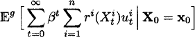
where is the initial starting state of all bandit processes and β (0,1) is the discount factor.

24.2.1 An Example

Consider an adaptive clinical trial with n treatment options. When the tth patient comes for treatment, she may be prescribed any one of the n available options based on the results of the previous trials. The sequence of success and failure of each treatment is an Bernoulli process with an unknown success probability sⁱ, i = 1, …, n. The objective is to design an adaptive strategy that maximizes the expected total discounted successful treatments.

The above adaptive clinical trial may be viewed as a MAB problem as follows. Suppose the prior distribution of sⁱ has a beta distribution that is independent across treatments. Then the posterior distribution of sⁱ, which is calculated using Bayes’ rule, is also a beta distribution, say Beta(p_tⁱ, q_tⁱ) at time t. Therefore, each treatment may be modeled as a Markovian bandit process where the state X_tⁱ is (p_tⁱ, q_tⁱ), the state update function f corresponds to Bayes update of the posterior distribution, and the reward function captures the probability of success.

24.2.2 Solution Concept and the Gittins Index

One possible solution concept for the MAB problem is to set it up as a Markov decision process (MDP) and use Markov decision theory [26] to solve it. However, such an approach does not scale well with the number of bandit processes because of the curse of dimensionality. To see this. assume that the state space ⁱ of each bandit process is a finite set with m elements. Then the state space of the resultant MDP, which is the space of realizations of X_t, has size mⁿ. The solution complexity of solving a MDP is proportional to the size of the state space. Hence the complexity of solving MAB using Markov decision theory increases exponentially with the number of bandit processes. A key breakthrough for the MAB problem was provided by Gittins and Jones [13] and Gittins [15], who showed that instead of solving the n-dimensional MDP with state-space Π_i=1^{n i}, an optimal solution is obtained by solving n 1-dimensional optimization problems: for each bandit i, 1 = 1, …, n, and for each state x^{i i}, compute.

(1)

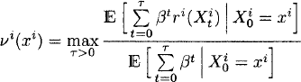
where τ is a measurable stopping time. The function vⁱ(xⁱ) is called Gittins index of bandit process i at state xⁱ. The optimal τ in (1), which is called the optimal stopping time at xⁱ, is given by the hitting time T(S(xⁱ)) of a stopping set , that is, the first time the bandit process enters the set S(xⁱ). Algorithms to compute the Gittins index of a bandit process are presented in Section 24.3.

Gittins and Jones [13] and Gittins [15] characterized the optimal strategy as follows:

• At each time, play the arm with the highest Gittins index.

Thus, to implement the optimal strategy, compute and store the Gittins index vⁱ(xⁱ) of all states x^{i i} of all bandit processes i, i = 1, …, n. Off-line algorithms that compute the Gittins index of all states of a bandit process are presented in Section 24.3.

An equivalent interpretation of the Gittins index strategy is the following:

• Pick the arm with the highest Gittins index and play it until its optimal stop ping time (or equivalently, until it enters the corresponding stopping set) and repeat.

Thus, an alternative way to implement the optimal strategy is to compute the Gittins index vⁱ(x_tⁱ) and the corresponding stopping time [or equivalently, the corresponding stopping set S(xⁱ)] for the current state x_tⁱ of all bandit processes i, i = 1, …., n. On-line algorithms that compute the Gittins index and the corresponding stopping set for an arbitrary state of a bandit process are presented in Section 24.4.

Off-line implementation is simpler and more convenient for bandit processes with finite and moderately sized state space. On-line implementation becomes more convenient for bandit processes with large or infinite state space.

24.2.3 Salient Features of the Model

As explained by Gittins [15], MAB problems admit a simpler solution than general multistage decision problems because they can be optimally solved with forward induction. In general, forward induction is not optimal and one needs to resort to backward induction to find the optimal strategy. Forward induction is optimal for MAB setup because it has the following features:

Because the above features, decisions made at each stage are not irrevocable and hence forward induction is optimal. On the basis of the above insight, Gittins [15] proved the optimality of the index strategy, using an interchange argument. Since then, various other proofs of the Gittins index strategy have been proposed (see [14] for a detailed summary).

Several variations of MAB problems have been considered in the literature. These variations remove some of the above features, and, as such, index strategies are not necessarily optimal for these variations. We refer the reader to the survey by Mahajan and Teneketzis [23] and references therein for details on the variations of the MAB problem.

24.3 Off-Line Algorithms for Computing Gittins Index

Since the Gittins index of a bandit process depends just on that process, we drop the label i and denote the bandit process by .

Off-line algorithms use the following property of the Gittins index. The Gittins index v : → induces a total order on that is given by

Using this total order, for any state a , the state space may be split into two sets

These sets are, respectively, called the continuation set and the stopping set. The rationale behind the terminology is that if we start playing a bandit process in state a. then it is optimal to continue playing the bandit process in all states C(a) because for any b C(a), v(b) > v(a). Thus, the stopping time that corresponds to starting the bandit process in state a is the hitting time T(S(a)) of set S(a), that is, the first time the bandit process enters set S(a). Using this characterization, the expression for Gittins index (1) simplifies to

(2)

where T(S(a)) = inf{t > 0 : X_t S(a)} is the hitting time of set S(a). The off-line algorithms use this simplified expression to compute the Gittins index.

For ease of exposition, assume that X_t takes values in a finite space = {1, …, m}. Most of the algorithms extend to countable state spaces under appropriate conditions. Denote the m × m transition probability matrix corresponding to the Markovian update of the bandit process by P = [P_{a, b}] and represent the reward function using a m × 1 vector r, i.e. r_a = r(a). Furthermore, let 1 be the m × 1 vector of ones, 0_{m × 1} be the m × 1 vector of zeros, I be the m × m identity matrix, and 0_m×m be the m × m matrix of zeros.

24.3.1 Largest-Remaining-Index Algorithm (Varaiya, Walrand, and Buyukkoc)

Varaiya, Walrand. and Buyukkoc [32] presented an algorithm to compute the Gittins index, which we refer to as the largest-remaining-index algorithm. The key idea behind this algorithm is to identify the states in according to the decreasing order

where (α₁, …, α_m) is a permutation of (1, …, m).

The algorithm proceeds as follows:

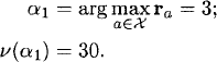
Initialization: The first step of the algorithm is to identify the state α₁ with the highest Gittins index. Since α₁ has the highest Gittins index, S(α₁) = . Substituting this in (2), we get that v(α₁) = r(α₁) = r_α1. Then, choose

where ties are broken arbitrarily. The corresponding Gittins index is

Recursion step: After the states α₁, …, α_k−1 have been identified, the next step is to identify the state α_k with the kth largest Gittins index. Even though α_k is not known, we know that C(α_k) = {α₁, …, α_k−1} and S(α_k) = {α₁, …, α_k−1}. Substituting this in (2), we can compute v(α_k) as follows. Define the m × m matrix by ,

(3)

and define the m × 1 vectors:

(4)

Then, choose

where ties are broken arbitrarily. The corresponding Gittins index is

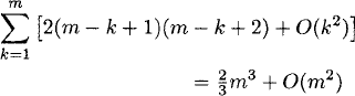
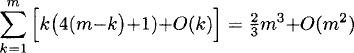
Computational complexity: The performance bottleneck of this algorithm is the two systems of the linear equations (4) that need to be solved at each step. At step k, each system effectively has k variables, so solving each requires (2/3)k³ + O(k²) arithmetic operations. Thus, overall this algorithm requires

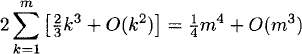
arithmetic operations. This algorithm has the worst computational complexity of all the algorithms presented.

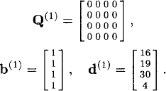
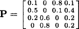
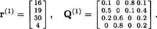
Example 24.3.1 Consider a bandit process with state space = {1,2,3,4}, reward vector r = [16 19 30 4]^T, and probability transition matrix

Let the discount factor be β = 0.75.

Using the largest-remaining-index algorithm, the Gittins index for this bandit process is calculated as follows:

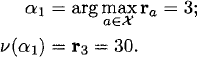
Initialization: Start by identifying the state with the highest Gittins index:

Recursion step:

1. Step k = 2: Although α₂ is not known, we know that C(α₂) = {3} and S(α₂) = {1, 2, 4}. Using (3) and (4) we get

Hence,

2. Step k = 3: Although α₃ is not known, we know that C(α₃) = {1, 3} and S(α₃) = {2, 4}. Using (3) and (4) we get

Hence,

3. Step k = 4: As before, although α₄ is not known, we know that C(α₄) = {1, 2, 3} and . As in the previous steps, using (3) and (4) we get

Since S(α₄) = {4} has only one element, we have

Thus, the vector of the Gittins index of this bandit process is

24.3.2 State-Elimination Algorithm (Sonin)

Sonin [30] presented an algorithm to compute the Gittins index, which we refer to as the state-elimination algorithm. As with the largest-remaining-index algorithm, the main idea behind the state-elimination algorithm is to iteratively solve (2) in the decreasing order of . The computations are based on a relation of (2) with optimal stopping problems [29].

A simplified version of the state-elimination algorithm is presented below. See [30] for a more efficient version that also works when the discount factor β depends on the state.

Initialization: The initialization step is identical to that of the largest-remaining-index algorithm: Identify the state α₁ with highest Gittins index, which is given by

where ties are broken arbitrarily. The corresponding Gittins index is

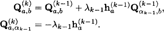
Step k of the recursion uses a × matrix Q^(k) and × 1 vectors d^(k) and b^(k), where . These are initialized as Q⁽¹⁾ = P, d⁽¹⁾ = r, and b⁽¹⁾ = (1 − β)1.

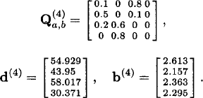
Recursion step: After the states α₁, …, α_k−1 have been identified, the next step is to identify the state α_k with the kth largest Gittins index. Even though α_k is not known, we know that and . Let the model in the step k − 1 be Q^(k−1), d^(k−1) and b^(k−1). Define

Let = |S(α_k)|. Define × matrix by :

(5)

and define × 1 vectors by

(6)

Note that the entries of Q^(k), d^(k) and b^(k) are labeled according to the set S(α_k). For example, if = {1, 2, 3}, α₁ = 2 then S(α₁) = {1,3} and

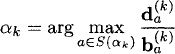
After calculating Q^(k), d^(k) and b^(k), choose

where ties are broken arbitrarily. The corresponding Gittins index is

Computational complexity: The performance bottleneck of this algorithm is the update of matrix Q^(k) at each step. In step k, the matrix Q^(k) has (m −k + 1)² elements and update of each element requires 2 arithmetic operations [since we can pre-compute , for all a S(α_k) before updating Q^(k)]. Thus, overall this algorithm requires

arithmetic operations. Our calculations differ from the m³ + O(m²) calculations reported in [24] because [24] assumes that the update of each element of Q^(k) takes 3 arithmetic operations, but, as we argued above, this update can be done in 2 operations if we pre-multiply row α_k−1 of Q^(k−1) with λ_k−1. Furthermore, in the implementation presented in [24], b^(k) is computed from Q^(k), requiring additional O(m²) arithmetic operations. The above implementation avoids those by keeping track of b^(k).

Example 24.3.2 Reconsider the bandit process of Example 24.3.1. Using the state-elimination algorithm, the Gittins index for this bandit process is calculated as follows.

Initialization: Start by identifying the state with the highest Gittins index:

Initialize:

Recursion step:

1. Step k = 2: Although α₂ is not known, we know that C(α₂) is {3}, S(α₂) = {1, 2, 4}, and λ₁ = β/(1 − = 0.75. Using (5) and (6) we get

Hence,

2. Step k = 3: Although α₃ is not known, we know that C(α₃) = {1, 3}, S(α₃) = {2, 4}, and λ₂ = β/(1 − = 0.898. Using (5) and (6) we get

Hence,

3. Step k = 4: Although α₄ is not known, we know that C(α₄) = {1, 2, 3}, S(α₄) = {4}, and λ₃ = 0.882. As in the previous steps, using (5) and (6) we get

Since S(α₄) = {4} has only one element, we have

24.3.3 Triangularization Algorithm (Denardo, Park, and Rothblum)

Denardo, Park, and Rothblum [12], independently of Sonin, presented an algorithm that is similar to the state-elimination algorithm. We refer to this algorithm as the triangularization algorithm. Although the main motivation for this algorithm was to compute the performance of any index strategy, it can be used to compute the Gittins index as well.

A slightly modified version of the triangularization algorithm is presented below. See [12] for the original version.

Initialization: The initialization step is identical to the previous two algorithms: Identify the state α₁ with the highest Gittins index, which is given by

where ties are broken arbitrarily. The corresponding Gittins index is

The recursion step uses a m × (m + 2) tableau

where Q^(k) is a m × m square matrix and d^(k) and b^(k) are m × 1 vectors. Initialize these as Q⁽¹⁾ = I − βP, d⁽¹⁾ = r, and b⁽¹⁾ = (1 − β)1.

Recursion step: After the states α₁, …, α_k−1 have been identified, the next step is to identify the state α_k with the kth largest Gittins index. As before, even though α_k is not known, we know that and . Suppose the tableau in step k − 1 is

Update this tableau using the following elementary row operations

1. Let . Scale row α_k−1 of tableau M^(k−1) by λ_k−1 [i.e., rescale row α_k−1 such that the (α_k−1, α_k−1) entry of M^(k−1) is 1].

2. For each state a S(α_k), subtract row α_k−1 times the constant from row a [these operations set to 0 for b C(α_k)]. The updated tableau is M^(k).

After updating the tableau, choose

where ties are broken arbitrarily. The corresponding Gittins index is

Computational complexity: The performance bottleneck of this algorithm is the elementary row operations performed at each step to update the tableau. In step k, this algorithm performs (m − k + 2) row operations and each row operation requires 2(m − k + 1) arithmetic operations [This is because columns corresponding to C(α_k−1) need not be updated because is 0]. Thus, overall the algorithm requires

arithmetic operations.

Example 24.3.3 Reconsider the bandit process of Example 24.3.1. Using the triangularization algorithm, the Gittins index for this bandit process is calculated as follows:

Initialization: As in the other two algorithms, the state with the highest Gittins index is

Initialize the tableau M⁽¹⁾ as

Recursion step:

1. Step k = 2: Since α₁ = 3, set = 1. Using the elementary row operations, the tableau M⁽²⁾ is updated to

2. Step k = 3: Since α₂ = 1, set = 1.198. Using the elementary row operations, the tableau M⁽³⁾ is updated to

3. Step k = 4: Since α₃ = 2, set = 1.189. Using the elementary row operations, the tableau M⁽⁴⁾ is updated to

24.3.4 Fast-Pivoting Algorithm (Niño-Mora)

Niño-Mora [24] presented an algorithm to compute the Gittins index that refines a previous algorithm proposed by Kallenberg [16]. We refer to this algorithm as the fast-pivoting algorithm. As with the other algorithms, the main idea behind the fast-pivoting algorithm is to iteratively solve (2) in the decreasing order of . The computations are based on a relation of (3) with marginal productivity rate [24].

A modified version of the algorithm is presented below. See [24] for the original version.

Initialization: The initialization step is identical to the previous three algorithms: identify the state α₁ with the highest Gittins index, which is given by

where ties are broken arbitrarily. The corresponding Gittins index is

The recursion step uses a × m matrix Q^(k) and × 1 vectors b^(k) and d^(k), where = |S(α_k)| = m − k + 1. Initialize these as Q⁽¹⁾ = 0_m×m, b⁽¹⁾ = 1, d⁽¹⁾ = r.

Recursion step: After the states α₁, …, α_k−1 have been identified, the next step is to identify the state α_k with the kth largest Gittins index. Even though α_k is not known, we know that and . Let the model in the step k − 1 be Q^(k−1), b^(k−1) and d^(k−1) and let = |S(α_k)|.

Define the ( + 1) × 1 vector by ,

(7)

Let

Define the × m matrix by and ,

(8)

and the × 1 vectors by

(9)

(10)

After the model has been updated, choose

and the corresponding Gittins index is given by

Computational complexity: The performance bottleneck of this algorithm is the calculation of h^(k−1) and the update of Q^(k), each of which requires 2(m – k + 2)k additions and multiplications [for the update of Q^(k), we know that for b S(α_k), Q^(k) is 0, hence we do not need to calculate those using (8)]. Thus, overall the algorithm requires

arithmetic operations.

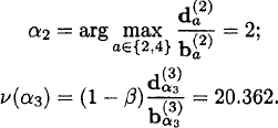
Example 24.3.4 Reconsider the bandit process of Example 24.3.1. Using the fast-pivoting algorithm, the Gittins index of this bandit process is computed as follows:

Initialization: As in the other two algorithms, the state with the highest Gittins index is

Initialize:

Recursion step:

24.3.5 An Efficient Method to Compute Gittins Index of Multiple Processes

Consider a MAB problem in which all processes have a finite state space i = {1, …, mi}. Let αmii be the state with the smallest Gittins index in process i, i = 1, …, n. Let

be the process whose smallest Gittins index is the largest among all alternatives. Then, a Gittins index strategy will eventually settle on process i^* and play it forever.

Based on the above insight, Denardo, Feinberg, and Rothblum [11] proposed the following method to efficiently compute the Gittins index of multiple processes in parallel.

Initialization: Identify the state α₁ⁱ with the highest Gittins index for all processes and calculate its Gittins index vⁱ(α₁ⁱ) (using any of the methods described above).

Recursion step: Suppose we have computed the Gittins index of the kⁱth highest state of process i, i = 1, …, n. Let

(11)

If k^j < m^j, then identify the state with the next highest Gittins index in process j (using any one of the methods described above), compute the Gittins index of that state, set k^j = k^j + 1, and repeat. Otherwise, if k^j = m^j, then j = i^* and we don’t need to compute the Gittins index of the remaining states as the Gittins index strategy will never play a process in those states (and instead prefers to play process i^*).

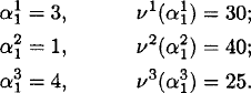
Example 24.3.5 To illustrate the above method, consider a MAB problem with three bandit processes, each with state space = {1, 2, 3, 4}. transition matrix

and reward vectors

Let the discount factor be β = 0.75. Note that the first bandit process is identical to that which we have considered in the previous examples. Using the above method, we proceed as follows:

Initialization: Compute the state with the highest Gittins index for each of the processes to get:

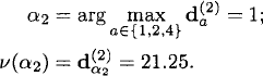
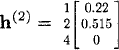
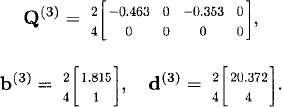
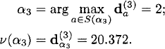
Recursion step:

24.4 On-Line Algorithms for Computing Gittins Index

As in the case of off-line algorithms, we consider a single bandit process and drop the label i of the bandit processes. For ease of exposition, assume that X_t takes value in a finite space = {1, …, m}. These algorithms are based on dynamic programming and linear programming and extend to countable state spaces based on standard extensions of dynamic and linear programming to countable state spaces. As before, denote the m × m transition probability matrix by P = [P_{a, b}] and represent the reward function using a m × 1 vector r. Furthermore, let 1 denote the m × 1 vector of ones and 0_m×1 denote the m × 1 vector of zeros.

On-line algorithms for Gittins index are based on bandit processes with the retirement option introduced by Whittle [34]. In such a bandit process, a player has the option to either play a regular bandit process and receive a reward according to the reward function r or choose to retire and receive a one-time retirement reward of M. Thus, the player is faced with an optimal stopping problem of maximizing

over all {σ(X₁, …, X_t)}_t=0^∞ measurable stopping times τ.

For a fixed value of retirement reward, an optimal solution is given by the solution of the following dynamic program. Let the m × 1 vector v^(M) be the unique fixed point of

(12)

where the max is element-wise maximum of two vectors. Standard results in Markov decision theory [26] show that the above equation has a unique point.

Fix a state α and let M_α denote the smallest retirement reward such that a player is indifferent between playing the bandit process starting at α or retiring, that is,

(13)

Whittle [34] showed that

(14)

The on-line algorithms use this interpretation to compute the Gittins index of a particular state α.

24.4.1 Restart Formulation (Katehakis and Veinott)

Katehakis and Veinott [18] related Whittle’s retirement option to a restart problem and then solved it using dynamic programming. The intuition behind their approach is the following. Fix a state α . When the retirement reward is M_α, the player is indifferent between playing the bandit process starting in state α or retiring. Therefore the option of retirement reward of M_α is equivalent to the option of restarting in state α.

On the basis of the above equivalence, consider the following restart problem. At each time, the player has an option to play the bandit process or instantaneously restart in state α. To describe a solution of this restart problem, define r⁽⁰⁾ = r_α1 and Q⁽⁰⁾ as

to be the instantaneous reward and transition probability matrix for the restart option and r⁽¹⁾ = r and Q⁽¹⁾ = P to be the instantaneous reward and transition matrix for the continuation option. Then a solution to the restart problem is given by the following dynamic program. Let the m × 1 vector v be the unique fixed point of

(15)

where max is the element-wise maximum of two vectors. Then the Gittins index of state α is

and the corresponding stopping set is

The fixed point equation (15) depends on the state α [because r⁽⁰⁾ and Q⁽⁰⁾ depend on α]. This equation may be solved using standard tools for solving dynamic programs such as value iteration, policy iteration, or dynamic programming. Beale (in the discussion of [15]) proposes an online algorithm that can be viewed as a special form of policy iteration to solve (15). See [26] for details on numerically solving fixed point equations for the form (15).

Example 24.4.1 Reconsider the bandit process of Example 24.3.1. To compute the Gittins index of state 2 (which is the state with the third largest index), proceed as follows:

Define

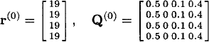
and

The dynamic program for the restart formulation is given by (15).

As mentioned above, there are various algorithms such as value iteration, policy iteration, linear programming, etc. to solve the above dynamic program. Using any one of these algorithms gives that

is the unique fixed point of (15). Hence

and

24.4.2 Linear Programming Formulation (Chen and Katehakis)

Chen and Katehakis [10] showed that M_α given by (13) may be computed using a linear program. A modified version of this linear program is presented below.

Define h = 1 − e_α, where e_α is the m × 1 unit vector with 1 at the αth position. Let diag(h) denote the m × m diagonal matrix with h as its diagonal. Let the (m + 1) × 1 vector z = [y^T | z]^T, where y is a m × 1 vector and z is a scalar, be the solutions of the following linear program.

subject to

(16)

Then the Gittins index of state α is

and the corresponding stopping set is

The linear program (16) depends on the state α (because h depends on α). This linear program may be solved using standard tools. See [6] for details.

Example 24.4.2 Reconsider the bandit process of Example 24.3.1. To compute the Gittins index of state 2 (which is the state with the third largest index), proceed as follows:

Define h = [1 1 0 1]^T. Let z = [y^T | z]^T be the solution to the following linear program:

(17)

subject to

As mentioned above, there are various algorithms to solve linear programs. Using any of these algorithms gives that

is the unique optimal solution of (17). Hence,

and

24.5 Computing Gittins Index for the Bernoulli Sampling Process

In clinical trials, it is common for treatments to be modeled as a Bernoulli process with unknown success probability sⁱ, i = 1, …, n. Such a MAB setup is called a Bernoulli sampling process because the player must sample from one of the n available Bernoulli processes at each time. Assume that sⁱ has a Beta(p₀ⁱ, q₀ⁱ) distribution¹ where p₀ⁱ and q₀ⁱ are nonnegative integers. Suppose at time t, sampling process i has resulted in k successes and failures. Then, the posterior distribution of sⁱ is Beta(p_tⁱ, q_tⁱ) where

Therefore, X_tⁱ (p_tⁱ, q_tⁱ) may be used as an information state (or a sufficient statistic) for the bandit process i. This state evolves in a Markovian manner. In particular if X_tⁱ = (p_tⁱ, q_tⁱ) then

where w.p. is an abbreviation for “with probability.” The average reward on playing process i is the mean value of Beta(p_tⁱ, q_tⁱ), that is,

In this section, we describe the various algorithms to compute the Gittins index of such a Bernoulli sampling process. As before, since the computation of the index depends only on that process, we drop the label i and denote the sampling process by and its Gittins index by v(p, q).

The main difficulty in computing the Gittins index v(p, q) is that the state space = ₊² is countably infinite. Hence, an exact computation of the index is not possible. In this section we present algorithms that compute the Gittins index with arbitrary precision by restricting to a truncated state space _L = {(p, q) | p + q ≤ L} for sufficiently large value of L. The results based on these calculations are tabulated in [14]. Different approximations to v(p, q) have also been proposed in the literature, and we describe a few of these in this section as well.

24.5.1 Dynamic Programming Formulation (Gittins)

Gittins [14] used the dynamic programming formulation of Whittle’s retirement option [34], which was presented in Section 24.4, to compute the Gittins index v(p, q). In the case of a Bernoulli sampling process, the dynamic program (12) simplifies to

(18)

where

Let M_p,q be defined as in (13). Then, the Gittins index is given by

Gittins [14] presents an approximate solution of (18) by restricting to _L = {(p, q) | p + q ≤ L}. discretizing M, and using value-iteration. On the basis of these calculations, the values of v(p, q) accurate up to four decimal places are tabulated in [14, Tables 8.4–8.8] for different values of β [0.5, 0.99]. MATLAB code for the above calculations is also available in [14].

Gittins [14] also observed that for large p + q the Gittins index v(p, q) is well approximated as follows: Let n = p + q and μ = p/n, then

where A, B, and C depend on β and μ. The fitted values of A, B, and C as a function of β and μ are tabulated in [14, Tables 8.9–8.11] for μ [0.025, 0.975] and β [0.5, 0.99].

24.5.2 Restart Formulation (Katehakis and Derman)

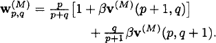
Katehakis and Derman [17] used the restart formulation of Katehakis and Veinott [18], which was presented in Section 24.4.1, to compute the Gittins index v(p, q). In the case of the Bernoulli sampling process, the dynamic program (15) for computing the Gittins index of a state (p₀, q₀) simplifies to

(19)

where

and w_p0,q0 is defined similarly. Katehakis and Derman presented an approximate solution of (19) by restricting to _L = {(p, q) | p + q ≤ L}. They also showed that for any ε > 0, there exists a sufficiently large L = L(ε) such that L iterations of value-iteration on the truncated state space _L gives a value function that is within ε of the true value function (Ben-Israel and Flåm [3] had derived similar similar bounds on value iteration for computing the Gittins index to a specific precision). Thus, this method may be used to calculate the Gittins index to an arbitrary precision.

24.5.3 Closed-Form Approximations

For large values of β, v(p, q) of a Bernoulli process may be approximated using diffusion approximation and using the Gittins index for a Weiner process. Two such closed-form approximations are presented below.

An important result in the context of these approximation is by Katehakis and Veinott [18], who showed that if we follow an index strategy where the index is within ε of the Gittins index, then the performance of the index strategy is within ε of the optimal performance.

Whittle’s approximation: Whittle [35] showed that for large p + q and β, the Gittins index of a Bernoulli sampling process may be approximated as

where n = p + q, μ = p/n, and c = ln β⁻¹.

Brezzi and Lai’s approximation: Brezzi and Lai [8] showed that the Gittins index of a Bernoulli sampling process may be approximated as

where μ and σ² are the mean and variance of Beta(p, q) distribution, that is,

(20)

ρ² is the variance of Bernoulli(μ) distribution, that is,

and >(s) is a nondecreasing, piecewise nonlinear function given by

Using the notation n = p + q, μ = p/n, and c = ln β⁻¹ the above expression simplifies to

This closed-form expression provides a good approximation for β ≥ 0.8 and min(p, q) ≥ 4.

24.5.4 Qualitative Properties of Gittins Index

Kelly [19] showed that the Gittins index is nondecreasing with the discount factor β. Brezzi and Lai [7] showed that

where μ and σ² are the mean and variance of Beta(p, q) distribution as given by (20). Bellman [2] showed that

Thus, the optimal strategy has the stay-on-the-winner property defined by Robbins [27].

As p + q → ∞, Kelly [19] showed that

where s is the true success probability of the Bernoulli process. The rate of convergence slows down as β → 1.

Kelly [19] showed that for any k > 0, there exists a sufficiently large β^* such that for β > β^*

Therefore, as β → 1, the optimal strategy tends to the least failure strategy: Sample the process with the least number of failures and in case of ties select the process with the largest number of successes.

Brezzi and Lai [7] (and also Rothschild [28], Kumar and Varaiya [21], and Banks and Sundaram [1] in slightly different setups) have shown that the Gittins index strategy eventually chooses one process that it samples for ever, and there is a positive probability that the chosen process does not have the maximum sⁱ. Thus, there is incomplete learning when following the Gittins index strategy.

24.6 Conclusion

In this chapter, we have summarized various algorithms to compute the Gittins index. We began by considering general Markovian bandit processes and described off-line and on-line algorithms to compute the Gittins index. We then considered the Bernoulli sampling process, described algorithms that approximately compute the Gittins index, and presented closed-form approximations and qualitative properties of the Gittins index.

References

[1] J. S. Banks and R. K. Sundaram, Denumerable-armed bandits, Econometrica: Journal of the Econometric Society, vol. 60, no. 5, pp. 1071–1096, 1992.

[2] R. Bellman, A problem in the sequential design of experiments, Sankhy: The Indian Journal of Statistics, vol. 16, no. 3/4, pp. 221–229, 1956.

[3] A. Ben-Israel and S. Flåm, A bisection/successive approximation method for computing Gittins indices, Mathematical Methods for Operations Research, vol. 34, no. 6, pp. 411–422, 1990.

[4] D. Bergemann and J. Valimaki, Bandit problems, in The New Palgrave Dictionary of Economics, S. N. Durlauf and L. E. Blume, Eds. Macmillan Press, pp. 336–340, 2008.

[5] D. A. Berry, Adaptive clinical trials: the promise and the caution, Journal of Clinical Oncology, vol. 29, no. 6, pp. 606–609, 2011.

[6] D. Bertsekas and J. N. Tsitsiklis, Introduction to Linear Optimization. Athena Scientific, 1997.

[7] M. Brezzi and T. L. Lai, Incomplete learning from endogenous data in dynamic allocation, Econometrica, vol. 68, no. 6, pp. 1511–1516, 2000.

[8] M. Brezzi and T. L. Lai, Optimal learning and experimentation in bandit problems, Journal of Economic Dynamics and Control, vol. 27, no. 1, pp. 87–108, 2002.

[9] S. Bubeck and N. Cesa-Bianchi, Regret analysis of stochastic and nonstochastic multi-armed bandit problems, Foundations and Trends in Machine Learning, vol. 5, no. 1, pp. 1–122, 2012.

[10] Y. R. Chen and M. N. Katehakis, Linear programming for finite state multi-armed bandit problems, Mathematics of Operations Research, vol. 11, no. 1, pp. 180–183, 1986.

[11] E. V. Denardo, E. A. Feinberg, and U. G. Rothblum, The multi-armed bandit, with constraints, Annals of Operations Research, vol. 208, pp. 37–62, 2013.

[12] E. V. Denardo, H. Park, and U. G. Rothblum, Risk-sensitive and risk-neutral multiarmed bandits, Mathematics of Operations Research, pp. 374–396, 2007.

[13] J. C. Gittins and D. M. Jones, A dynamic allocation index for the discounted multiarmed bandit problem, in Progress in Statistics, Amsterdam, Netherlands: North-Holland, vol. 9, pp. 241–266, 1974.

[14] J. Gittins, K. Glazebrook, and R. Weber, Multi-Armed Bandit Allocation Indices, Wiley, 2011.

[15] J. C. Gittins, Bandit processes and dynamic allocation indices, Journal of the Royal Statistical Society, Series B (Methodological), vol. 41, no. 2, pp. 148–177, 1979.

[16] L. C. Kallenberg, A note on MN Katehakis’ and Y.-R. Chen’s computation of the Gittins index, Mathematics of operations research, vol. 11, no. 1, pp. 184–186, 1986.

[17] M. N. Katehakis and C. Derman, Computing optimal sequential allocation rules in clinical trials, Lecture Notes-Monograph Series, vol. 8, pp. 29–39, 1986.

[18] M. N. Katehakis and A. F. Veinott, The multi-armed bandit problem: decomposition and computation, Mathematics of Operations Research, vol. 12, no. 2, pp. 262–268, 1987.

[19] F. Kelly, Multi-armed bandits with discount factor near one: The Bernoulli case, The Annals of Statistics, vol. 9, no. 5, pp. 987–1001, 1981.

[20] V. Kuleshov and D. Precup, Algorithms for the multi-armed bandit problem, Journal of Machine Learning Research, vol. 1, pp. 1–48, 2000.

[21] P. R. Kumar and P. Varaiya, Stochastic Systems: Estimation Identification and Adaptive Control, Prentice Hall, 1986.

[22] T. L. Lai and H. Robbins, Asymptotically efficient adaptive allocation rules, Advances in applied mathematics, vol. 6, no. 1, pp. 4–22, 1985.

[23] A. Mahajan and D. Teneketzis, Foundations and Applications of Sensor Management, ch. Multi-armed bandits, Springer-Verlag, pp. 121–151, 2008.

[24] J. Niño-Mora, A (2/3)n³ fast-pivoting algorithm for the Gittins index and optimal stopping of a Markov chain, INFORMS Journal on Computing, vol. 19, no. 4, pp. 596–606, 2007.

[25] J. Nino-Mora, Stochastic scheduling. Encyclopedia of Optimization, vol. 5, pp. 367–372, 2009.

[26] M. Puterman, Markov Decision Processes: Discrete Stochastic Dynamic Programming, John Wiley and Sons, 1994.

[27] H. Robbins, Some aspects of the sequential design of experiments, Bulletin of American Mathematics Society, vol. 58, pp. 527–536, 1952.

[28] M. Rothschild, A two-armed bandit theory of market pricing, Journal of Economic Theory, vol. 9, no. 2, pp. 185–202, 1974.

[29] I. Sonin, The elimination algorithm for the problem of optimal stopping, Mathematical methods of operations research, vol. 49, no. 1, pp. 111–123, 1999.

[30] I. M. Sonin, A generalized Gittins index for a Markov chain and its recursive calculation, Statistics & Probability Letters, vol. 78, no. 12, pp. 1526–1533, 2008.

[31] W. R. Thompson, On the likelihood that one unknown probability exceeds another in view of the evidence of two samples, Biometrika, vol. 25, no. 3/4, pp. 285–294, 1933.

[32] P. Varaiya, J. Walrand, and C. Buyukkoc, Extensions of the multiarmed bandit problem: the discounted case, IEEE Trans. Autom. Control, vol. 30, no. 5, pp. 426–439, 1985.

[33] R. B. Washburn, Application of multi-armed bandits to sensor management, in Foundations and Applications of Sensor Management. Springer, pp. 153–175, 2008.

[34] P. Whittle, Multi-armed bandits and the Gittins index, Journal of the Royal Statistical Society, Series B (Methodological), vol. 42, no. 2, pp. 143–149, 1980.

[35] P. Whittle, Optimization Over Time, ser. Wiley Series in Probability and Mathematical Statistics, vol. 2, John Wiley and Sons, 1983,.

[36] Y. Wu, W. J. Shih, and D. F. Moore, Elicitation of a beta prior for bayesian inference in clinical trials, Biometrical Journal, vol. 50, no. 2, pp. 212–223, 2008.

¹If a random variable s has Beta(p, q) distribution, then its PDF (probability density function) f(s) is proportional to s^p(1 – s)^q. See [36] for methods to elicit Beta priors based on expert opinions in clinical trials.