
Chapter 11
Building descriptive statistical formulas
In this chapter, you will:
Understand descriptive statistics
Learn how to count items and calculate permutations and combinations
Calculate the mean, median, mode, and other averages
Work with maximums, minimums, and other extreme values
Calculate measures of variation such as the range, variance, and standard deviation
In Excel’s list of worksheet functions, the Statistical category boasts well over 100 functions. That’s a massive number, and it inevitably means that many of those functions are obscure and highly specialized. That’s great if you’re a specialist, but for general business uses it’s highly unlikely you’ll ever need the Fisher transformation (via the FISHER() function), the Pearson product moment coefficient correlation (via the PEARSON() function), or the value of the density function for a standard normal distribution (via the PHI() function).
That’s not to say there aren’t useful statistical functions for business. Quite the opposite: Excel is chock-full of statistical functions that are both powerful and useful in a business context. When building your Excel worksheet models, you’ll need to count things, calculate averages, look for extreme values, calculate measures of variation, and more. You learn how to do all that and more in this chapter, and you explore even more statistical functions in Chapter 12, “Building inferential statistical formulas,” and 13, “Applying regression to track trends and make forecasts.”
Understanding descriptive statistics
One of the goals of this book is to show you how to use formulas and functions to turn a jumble of numbers and values into results and summaries that give you useful information about the data. Excel’s statistical functions are particularly useful for extracting analytical sense out of data nonsense. Many of these functions might seem strange and obscure, but they reward a bit of patience and effort with striking new views of your data.
This is particularly true of the branch of statistics known casually as descriptive statistics (or summary statistics). As the name implies, you use descriptive statistics to describe various aspects of a data set, so you get a better overall picture of the phenomenon underlying the numbers. In Excel’s statistical repertoire, the following measures make up its descriptive statistics package: sum, count, mean, median, mode, maximum, minimum, kth largest, kth smallest, rank, percentile, range, standard deviation, variance, covariance, frequency distribution, kurtosis, and skewness.
In this chapter, you learn how to wield all these statistical measures (except sum, which I cover earlier in this book in Chapter 9, “Working with math functions”). The context is the worksheet database of product inventory shown in Figure 11-1.

Counting items
The simplest of the descriptive statistics is the total number of values in a data set. However, that simplicity isn’t reflected in Excel’s worksheet functions, which offer no less than five count-related functions. The next five sections take a quick look at each of Excel’s counting functions.
The COUNT() function
To count only the numeric values in a data set (that is, to ignore text values, dates, logical values, and errors), use the COUNT() function:
COUNT(value1[,value2,...])
value1, value2,... |
One or more ranges, arrays, function results, expressions, or literal values of which you want the count |
In the table shown in Figure 11-1, you can count the number of products in the table by using the following formula to count the numeric values in the Quantity column:
=COUNT(D4:D27)
![]() Tip
Tip
To get a quick look at the count, select the range or, if you’re working with data in a table, select a single column in the table. Excel displays the count in the status bar. If you want to know how many numeric values are in the selection, right-click the status bar and then select the Numerical Count value.
The COUNTA() function
To count not only the numeric values that appear in a data set but also the text values, dates, logical values, and errors, use the COUNTA() function:
COUNTA(value1[,value2,...])
value1, value2,... |
One or more ranges, arrays, function results, expressions, or literal values of which you want the count |
In the table shown in Figure 11-1, you can count the total number of rows in the table by using the following formula to count the values in the Quantity column, including the column header (cell D3):
=COUNTA(D3:D27)
The COUNTBLANK() function
To count the empty cells in a data set, use the COUNTBLANK() function:
COUNTBLANK(value1[,value2,...])
value1, value2,... |
One or more ranges, arrays, function results, expressions, or literal values of which you want the count |
In the table shown in Figure 11-1, you can use the following formula to count the number of blank cells in the Code column:
=COUNTBLANK(A4:A27)
The COUNTIF() function
The COUNTIF() function counts the number of cells in a range that meet a single criteria:
COUNTIF(range, criteria)
range |
The range of cells to use for the count. |
criteria |
The criteria, entered as text, that determines which cells to count. Excel applies the criteria to range. |
For example, in the table shown in Figure 11-1, you can use the following formula to count the number of products for which the Quantity is greater than or equal to 100:
=COUNTIF(D4:D27, ">= 100")
The COUNTIFS() function
The COUNTIFS() function counts the number of cells in one or more ranges that meet one or more criteria:
COUNTIFS(range1, criteria1[, range2, criteria2, ...])
range1 |
The first range of cells to use for the count. |
criteria1 |
The first criteria, entered as text, that determines which cells to count. Excel applies the criteria to range1. |
range2 |
The second range of cells to use for the count. |
criteria2 |
The second criteria, entered as text, that determines which cells to count. Excel applies the criteria to range2. |
You can enter up to 127 range/criteria pairs, and Excel only counts those cells that match all the criteria. For example, in the table shown in Figure 11-1, you can use the following formula to count the number of products where the Cost is greater than $30 and the Quantity is less than 50:
=COUNTIF(C4:C27, "> 30", D4:D27, "< 50")
Calculating averages
The most basic statistical analysis worthy of the name is probably the average, although you always need to ask yourself which average you need: mean, median, or mode. The next few sections show you the worksheet functions that calculate them.
The AVERAGE() function
The mean is what you probably think of when someone uses the term average. That is, it’s the arithmetic average of a set of numbers. In Excel, you calculate the mean by using the AVERAGE() function:
AVERAGE(number1[,number2,...])
number1, number2,... |
A range, an array, or a list of values of which you want the mean |
For example, to calculate the mean of the values in the Quantity field of the table shown earlier in Figure 11-1, use the following formula:
=AVERAGE(D4:D27)
![]() Tip
Tip
If you need just a quick glance at the mean value, select the range. Excel displays the average in the status bar.
![]() Caution
Caution
The AVERAGE() function (as well as the MEDIAN() and MODE() functions discussed in the next two sections) ignores text and logical values. It also ignores blank cells, but it does not ignore cells that contain the value 0. If you want to include non-numeric values, use the AVERAGEA() function, which treats text values as 0 and the Boolean values TRUE and FALSE as 1 and 0, respectively.
The AVERAGEIF() function
The AVERAGEIF() function calculates the average of a data set for those items that meet a specified condition:
AVERAGEIF(range, criteria[, average_range])
range |
The range of cells to use for the criteria. |
criteria |
The criteria, entered as text, that determines which cells to average. Excel applies the criteria to range. |
average_range |
The range from which the average values are taken. Excel averages only those cells in average_range that correspond to the cells in range and meet the criteria. If you omit average_range, Excel uses range for the average. |
For example, in the table shown earlier in Figure 11-1, you can use the following formula to calculate the average Quantity value for those products where the Cost field is greater than $25:
=AVERAGEIF(C4:C27, "> 25", D4:D27)
The AVERAGEIFS() function
The AVERAGEIFS() function averages cells in one or more ranges that meet one or more criteria:
AVERAGEIFS(average_range, range1, criteria1[, range2, criteria2, ...])
average_range |
The range from which the average values are taken. Excel averages only those cells in average_range that correspond to the cells that meet the criteria. |
range1 |
The first range of cells to use for the average criteria. |
criteria1 |
The first criteria, entered as text, that determines which cells to average. Excel applies the criteria to range1. |
range2 |
The second range of cells to use for the average criteria. |
criteria2 |
The second criteria, entered as text, that determines which cells to average. Excel applies the criteria to range2. |
You can enter up to 127 range/criteria pairs, and Excel only averages those cells that match all the criteria. For example, in the table shown earlier in Figure 11-1, you can use the following formula to calculate the average Quantity value where the Cost is greater than $30 and less than $50:
=AVERAGEIFS(D4:D27, C4:C27, "> 30", C4:C27, "< 50")
The MEDIAN() function
The median is the value in a data set that would fall in the middle if you sorted the values in numeric order. That is, 50% of the values fall below the median, and 50% fall above it. The median is useful in data sets that have one or two extreme values that can throw off the mean result because the median isn’t affected by extremes.
You calculate the median by using the MEDIAN() function:
MEDIAN(number1[,number2,...])
number1, number2,... |
A range, an array, or a list of values of which you want the median |
For example, to calculate the median of the Quantity values in the Product Inventory table (refer to Figure 11-1), you use the following formula:
=MEDIAN(D4:D27)
The MODE() function
The mode is the value in a data set that occurs most frequently. The mode is useful when you’re dealing with data that doesn’t lend itself to being either added (necessary for calculating the mean) or sorted (necessary for calculating the median). For example, you might be tabulating the result of a poll that included a question about the respondent’s favorite color. The mean and median don’t make sense with such a question, but the mode will tell you which color was chosen the most.
You calculate the mode using one of the following functions:
MODE.MULT(number1[,number2,...])
MODE.SNGL(number1[,number2,...])
number1, number2,... |
A range, an array, or a list of values for which you want the mode |
The MODE.SNGL() function returns the most common value in the list, so it’s the function you’ll use most often. If your list has multiple common values, use MODE.MULT() to return those values as an array.
For example, to calculate the mode of the Quantity values in the Product Inventory table (refer to Figure 11-1), you use the following formula:
=MODE.SNGL(D4:D27)
Calculating the weighted mean
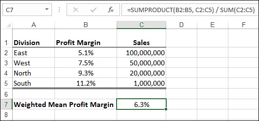
In some data sets, one value might be more important than another. For example, suppose that your company has several divisions, the biggest of which generates $100 million in annual sales and the smallest of which generates only $1 million in sales. If you want to calculate the average profit margin for the divisions, it doesn’t make sense to treat the divisions equally because the largest is two orders of magnitude bigger than the smallest. You need some way of factoring the size of each division into your average profit margin calculation.
You can do this by calculating the weighted mean. This is an arithmetic mean in which each value is weighted according to its importance in the data set. Here’s the general procedure to follow to calculate the weighted mean:
For each value, multiply the value by its weight.
Sum the results from step 1.
Sum the weights.
Divide the sum from step 2 by the sum from step 3.
This procedure works, but it requires building three extra calculations into your worksheet model: the products of the value-weight pairs, the sum of those products, and the sum of the weights. You can avoid all that extra work by using Excel’s SUMPRODUCT() function:
SUMPRODUCT(array1[,array2,...])
array1, array2,... |
The ranges or arrays you want to work with, each of which must have the same number of elements |
SUMPRODUCT() works by multiplying the corresponding items in each range or array (that is, the first items are multiplied, then the second items are multiplied, and so on) and then summing those products.
For example, Figure 11-2 shows a worksheet that lists the profit margin (B2:B5) and sales (C2:C5) for four divisions. Cell C7 uses the following formula to calculate the weighted mean profit margin:
=SUMPRODUCT(B2:B5, C2:C5) / SUM(C2:C5)
Calculating extreme values
The average calculations tell you things about the “middle” of the data, but it can also be useful to know something about the “edges” of the data. For example, what’s the biggest value, and what’s the smallest? The next two sections take you through the worksheet functions that return the extreme values of a data set.
The MAX() and MIN() functions
If you want to know the largest value in a data set, use the MAX() function:
MAX(number1[,number2,...])
number1, number2,... |
A range, an array, or a list of values of which you want the maximum |
For example, to calculate the maximum Quantity value in the Product Inventory table (refer to Figure 11-1), you use the following formula:
=MAX(D4:D27)
To get the smallest value in a data set, use the MIN() function:
MIN(number1[,number2,...])
number1, number2,... |
A range, an array, or a list of values of which you want the minimum |
For example, to calculate the minimum value in the Product Inventory table (refer to Figure 11-1), you use the following formula:
=MIN(D4:D27)
![]() Tip
Tip
If you need just a quick glance at the maximum or minimum value, select the range, right-click the status bar, and then click the Maximum or Minimum value.
![]() Note
Note
If you need to determine the maximum or minimum over a range or an array that includes text values or logical values, use the MAXA() or MINA() functions instead. These functions ignore text values and treat logical values as either 1 (for TRUE) or 0 (for FALSE).
The LARGE() and SMALL() functions
Instead of knowing just the largest value, you might need to know the kth largest value, where k is some integer. You can calculate this by using Excel’s LARGE() function:
LARGE(array, k)
array |
A range, an array, or a list of values. |
k |
The position (beginning at the largest) within array that you want to return. (When k equals 1, this function returns the same value as MAX().) |
For example, the following formula returns 120, the second-largest Quantity value in the Product Inventory table (refer to Figure 11-1):
=LARGE(D4:D27, 2)
Similarly, instead of knowing just the smallest value, you might need to know the kth smallest value, where k is some integer. You can determine this value by using the SMALL() function:
SMALL(array, k)
array |
A range, an array, or a list of values. |
k |
The position (beginning at the smallest) within array that you want to return. (When k equals 1, this function returns the same value as MIN().) |
For example, the following formula returns 15, the third-smallest Quantity value in the Product Inventory table (refer to Figure 11-1):
=SMALL(D4:D27, 3)
Performing calculations on the top k values
Sometimes, you might need to sum only the top three values in a data set or take the average of the top 10 values. You can do this by combining the LARGE() function and the appropriate arithmetic function (such as SUM()) in an array formula. Here’s the general formula:
=FUNCTION(LARGE(range, {1,2,3,...,k}))
Here, FUNCTION() is the arithmetic function, range is the array or range containing the data, and k is the number of values you want to work with. In other words, LARGE() applies the top k values from range to the FUNCTION().
For example, suppose you want to find the mean of the top five Quantity values in the Product Inventory table (refer to Figure 11-1). Here’s an array formula that does this:
=AVERAGE(LARGE(D4:D27,{1,2,3,4,5}))
Performing calculations on the bottom k values
You can probably guess that performing calculations on the smallest k values is similar to performing calculations on the top k values. In fact, the only difference is that you substitute the SMALL() function for LARGE() in the array formula:
=FUNCTION(SMALL(range, {1,2,3,...,k}))
For example, the following array formula sums the smallest three Quantity values in the Product Inventory table (refer to Figure 11-1):
=SUM(SMALL(D4:D27,{1,2,3}))
Working with rank and percentile
The MAX(), MIN(), LARGE(), and SMALL() functions examine a range and return the maximum, minimum, kth largest, and kth smallest value, respectively, in that range. These functions examine the forest and return a tree. The opposite technique, in a sense, is the trees-instead-of-forest approach: Given a cell within a range, you want to know where that cell’s value stands with respect to all the other values in that range. There are two measures you can use to examine a cell’s value in relation to the range values:
Rank: This is the position of the cell’s value if you were to sort the range in descending order. The largest value gets rank 1, the second-largest value gets rank 2, and so on.
Percentile: This is the percentage of items in the range that are at the same level or a lower level than the cell’s value.
Calculating rank
To calculate the rank, you can use one of the following functions:
RANK.AVG(number, ref[, order])
RANK.EQ(number, ref[, order])
number |
The number for which you want to find the rank. |
ref |
A reference, a range name, or an array that corresponds to the set of values in which number will be ranked. (Note that ref must include number.) |
order |
An integer that specifies how number is ranked within the set. If order is 0 (this is the default), Excel treats the set as though it were ranked in descending order; if order is any nonzero value, Excel treats the set as though it were ranked in ascending order. |
For example, the following formula returns the rank of cell D14 in the Product Inventory table (see Figure 11-1):
=RANK.AVG(D14, D4:D27)
With RANK.AVG(), if two or more cells in the range have the same value, Excel returns the average of their ranks. For example, given the values 50, 42, 37, 37, 25, 10, RANK.AVG() ranks both instances of 37 as 3.5, which is the average of 3 and 4. By contrast, RANK.EQ() would give both instances of 37 the rank 3. With both RANK.AVG() and RANK.EQ(), if two or more numbers have the same rank, subsequent ranks are affected. For example, in the preceding list, the number 25 ranks fifth.
Calculating percentile
To calculate the percentile, you can use one of the following functions:
PERCENTILE.EXC(array, k)
PERCENTILE.INC(array, k)
array |
A reference, a range name, or an array of values for the set of data. |
k |
The percentile, expressed as a decimal value between 0 and 1. This value can be 0 or 1 if you use PERCENTILE.INC(), but not if you use PERCENTILE.EXC(). |
For example, the following formula returns the Quantity value in the Product Inventory table (refer to Figure 11-1) that represents the 90th percentile:
=PERCENTILE.EXC(D4:D27, 0.9)
Calculating measures of variation
Descriptive statistics such as the mean, median, and mode fall under what statisticians call measures of central tendency (or sometimes measures of location). These numbers are designed to give you some idea of what constitutes a “typical” value in a data set.
Contrast this with the so-called measures of variation (or sometimes measures of dispersion), which are designed to give you some idea of how the values in a data set vary with respect to one another. That is, are the values spread out, bunched together, or something in between those extremes? For example, a data set in which all the values are the same would have no variability; in contrast, a data set with wildly different values would have high variability. Just what is meant by “wildly different” is what the statistical techniques in this section are designed to help you calculate.
Calculating the range
The simplest measure of variability is the range (also sometimes called the spread), which is defined as the difference between a data set’s maximum and minimum values. Excel doesn’t have a function that calculates the range directly. Instead, you first apply the MAX() and MIN() functions to the data set. Then, when you have these extreme values, you calculate the range by subtracting the minimum from the maximum.
For example, here’s a formula that calculates the range for the Quantity column of the Product Inventory table (refer to Figure 11-1):
=MAX(D4:D27) - MIN(D4:D27)
In general, the range is a useful measure of variation only for small sample sizes. The larger the sample is, the more likely it becomes that an extreme maximum or minimum (or both) will occur, and the range will be skewed accordingly.
Calculating the variance
When computing the variability of a set of values, one straightforward approach is to calculate how much each value deviates from the mean. You can then add those differences and divide by the number of values in the sample to get what might be called the average difference. The problem, however, is that, by definition of the arithmetic mean, adding the differences (some of which are positive and some of which are negative) gives the result 0. To solve this problem, you need to add the absolute values of the deviations and then divide by the sample size. This is what statisticians call the average deviation.
Unfortunately, this simple state of affairs is still problematic because (for highly technical reasons) mathematicians tend to shudder at equations that require absolute values. To get around this, they instead use the square of each deviation from the mean, which always results in a positive number. They sum these squares and divide by the number of values, and the result is then called the variance. This is a common measure of variation, although interpreting it is difficult because the result isn’t in the units of the sample: It’s in those units squared. What does it mean to speak of “quantity squared,” for example? This doesn’t matter that much for our purposes because, as I explain in the next section, the variance is used chiefly to get to the standard deviation.
![]() Note
Note
Keep in mind that this explanation of variance is simplified considerably. If you’d like to know more about this topic, you can consult an intermediate statistics book.
In any case, variance is usually a standard part of a descriptive statistics package, so that’s why I’m covering it. Excel calculates the variance by using the VAR.P() and VAR.S() functions:
VAR.P(number1[,number2,...])
VAR.S(number1[,number2,...])
number1, number2,... |
A range, an array, or a list of values of which you want the variance |
You use the VAR.P() function if your data set represents the entire population (as it does, for example, in the Product Inventory table; refer to Figure 11-1); you use the VAR.S() function if your data set represents only a sample from the entire population.
For example, to calculate the variance of the Quantity values in the Product Inventory table, you use the following formula:
=VAR.P(D4:D27)
![]() Note
Note
If you need to determine the variance over a range or an array that includes text values or logical values, use the VARPA() (for a population) or VARA() (for a sample) functions instead. These functions ignore text values and treat logical values as either 1 (for TRUE) or 0 (for FALSE).
Calculating the standard deviation
As I mentioned in the previous section, in real-world scenarios, the variance is really used only as an intermediate step for calculating the most important of the measures of variation: the standard deviation. This measure tells you how much the values in the data set vary with respect to the average (the arithmetic mean). What exactly this means won’t become clear until you learn about frequency distributions in the next section. For now, however, it’s enough to know that a low standard deviation means that the data values are clustered near the mean, and a high standard deviation means that the values are spread out from the mean.
The standard deviation is defined as the square root of the variance. This means that the resulting units will be the same as those used by the data. For example, the variance of the product quantity is expressed as the meaningless units squared value, but the standard deviation is expressed in units.
You could calculate the standard deviation by taking the square root of the VAR.P() or VAR.S() result, but Excel offers a more direct route:
STDEV.P(number1[,number2,...])
STDEV.S(number1[,number2,...])
number1, number2,... |
A range, an array, or a list of values of which you want the standard deviation |
You use the STDEV.P() function if your data set represents the entire population (as in the Product Inventory table; see Figure 11-1); you use the STDEV.S() function if your data set represents only a sample from the entire population.
For example, to calculate the standard deviation of the Quantity values in the Product Inventory table, you use the following formula:
=STDEV.P(D4:D27)
![]() Note
Note
If you need to determine the standard deviation over a range or an array that includes text values or logical values, use the STDEVPA() (for a population) or STDEVA() (for a sample) function instead. These functions ignore text values and treat logical values as either 1 (for TRUE) or 0 (for FALSE).
Working with frequency distributions
A frequency distribution is a data table that groups data values into bins—ranges of values—and shows how many values fall into each bin. For example, here’s a possible frequency distribution for the Product Inventory data (refer to Figure 11-1):
Bin (Quantity) |
Count |
0–75 |
19 |
76–150 |
4 |
151–225 |
0 |
225–300 |
0 |
301–375 |
1 |
The size of each bin is called the bin interval. How many bins should you use? The answer usually depends on the data. If you want to calculate the frequency distribution for a set of student grades, for example, you’d probably set up six bins: 0–49, 50–59, 60–69, 70–79, 80–89, and 90–100. For poll results, you might group the data by age into four bins: 18–34, 35–49, 50–64, and 65+.
If your data has no obvious bin intervals, you can use the following rule:
If n is the number of values in the data set, enclose n between two successive powers of 2 and take the higher exponent to be the number of bins.
For example, if n is 100, you’d use 7 bins because 100 lies between 26 (64) and 27 (128). For the Product Inventory table, n is 24, so the number of bins should be 5 because 24 falls between 24 (16) and 25 (32).
![]() Tip
Tip
Here’s a worksheet formula that implements the bin-calculation rule:
=CEILING(LOG(COUNT(input_range), 2), 1)
To help you construct a frequency distribution, Excel offers the FREQUENCY() function:
FREQUENCY(data_array, bins_array)
data_array |
A range or an array of data values |
bins_array |
A range or an array of numbers representing the upper bounds of each bin |
Here are some things you need to know about this function:
For the bins_array, you enter only the upper limit of each bin. If the last bin is open ended (such as 16+), you don’t include it in the bins_array. For example, here’s the bins_array for the Product Inventory table’s frequency distribution shown earlier: {75, 150, 225, 300, 375}.
![]() Caution
Caution
Make sure you enter your bin values in ascending order.
The FREQUENCY() function returns an array, where each item in the array is the number of values that fall within each bin.
Because FREQUENCY() returns an array, you must enter it as an array formula. To do this, select the range in which you want the function results to appear, type the formula, and select Ctrl+Shift+Enter.
Figure 11-3 shows the Product Inventory table with a frequency distribution added. The bins_array is the range I5:I9, and the FREQUENCY() results appear in the range J5:J9, with the following formula entered as an array in that range:
=FREQUENCY(D4:D27, I5:I9)
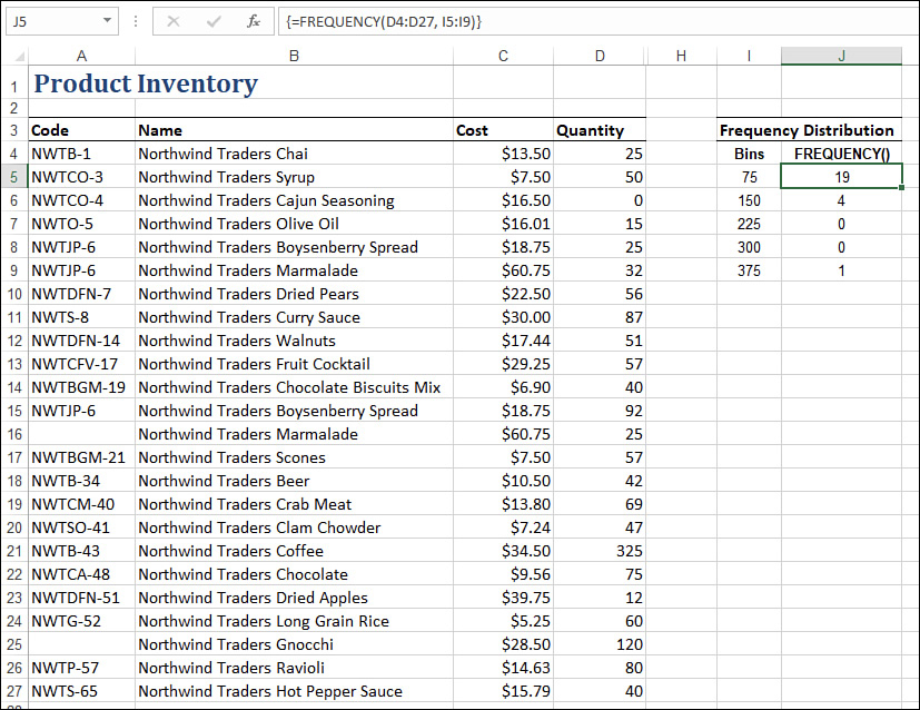
Figure 11-4 shows the final Product Inventory worksheet, including all the descriptive statistical values I discussed in this chapter.
