
Chapter 17
Analyzing data with tables
In this chapter, you will:
Use formulas to perform advanced table sorting
Use formulas to create advanced table filters
Learn how to reference table data in your formulas
Investigate Excel’s powerful database functions for analyzing table data
Excel’s forte is spreadsheet work, of course, but its row-and-column layout also makes it a natural database manager. In Excel, a table is a collection of related information with an organizational structure that makes it easy to find or extract data from its contents. Specifically, a table is a worksheet range that has the following properties:
Field: A single type of information, such as a name, an address, or a phone number. In Excel tables, each column is a field.
Field name: A unique name you assign to every table field. These names are always found in the first row of the table.
Field value: A single item in a field. In an Excel table, the field values are the individual cells.
Record: A collection of associated field values. In Excel tables, each row is a record.
Table range: The worksheet range that includes all the records, fields, and field names of a table.
In this chapter, I assume you know how to create, edit, and format tables, and how to perform basic table maintenance, so I don’t cover any of those things. Instead, I concentrate on using Excel formulas to help you analyze your table data.
Sorting a table
One of the advantages of a table is that you can rearrange its records so that they’re sorted alphabetically or numerically. This feature enables you to view the data in order by customer name, account number, part number, or any other field. You even can sort on multiple fields, which would enable you, for example, to sort a client table by state and then by name within each state.
For quick sorts on a single field, you have two choices to get started:
Select a cell anywhere inside the field and then select the Data tab.
Select the field’s Sort & Filter drop-down arrow.
For an ascending sort, select Sort A to Z (or Sort Smallest To Largest for a numeric field or Sort Oldest To Newest for a date field); for a descending sort, select Sort Z To A (or Sort Largest To Smallest for a numeric field or Sort Newest To Oldest for a date field).
![]() Caution
Caution
Be careful when you sort table records that contain formulas. If the formulas use relative addresses that refer to cells outside their own record, the new sort order might change the references and produce erroneous results. If your table formulas must refer to cells outside the table, be sure to use absolute addresses.
Sorting on part of a field
Excel performs its sorting chores based on the entire contents of each cell in a field. This method is fine for most sorting tasks, but occasionally you need to sort on only part of a field. For example, your table might have a ContactName field that contains a first name and then a last name. Sorting on this field orders the table by each person’s first name, which is probably not what you want. To sort on the last name, you need to create a new column that extracts the last name from the ContactName field. You can then use this new column for the sort.
Excel’s text functions make it easy to extract substrings from a cell. In this case, assume that each cell in the ContactName field has a first name, followed by a space, followed by a last name. Your task is to extract everything after the space, and the following formula does the job (assuming that the name is in cell D4):
=RIGHT(D4, LEN(D4) - FIND(" ", D4))
For an explanation of how this formula works, see “Extracting a first name or last name,” in Chapter 5, “Working with text functions.”
Figure 17-1 shows this formula in action. Column D contains the names, and column A contains the formula to extract the last name. I sorted on column A to order the table by last name.

![]() Tip
Tip
If you’d rather not have the extra sort field (column A in Figure 17-1) cluttering the table, you can hide it by selecting a cell in the field and selecting Home >Format > Hide & Unhide > Hide Columns. Fortunately, you don’t have to unhide the field to sort on it because Excel still includes the field in the Sort dialog box (select Data > Sort).
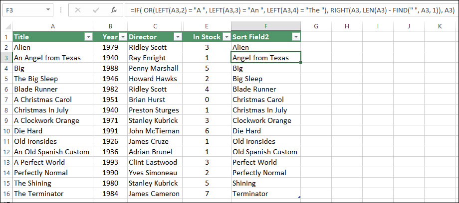
Sorting without articles
Tables that contain field values starting with articles (A, An, and The) can throw off your sorting. To fix this problem, you can borrow the technique from the preceding section and sort on a new field in which the leading articles have been removed. As before, you want to extract everything after the first space, but you can’t just use the same formula because not all the titles have a leading article. You need to test for a leading article by using the following OR() function:
OR(LEFT(A2,2) = "A ", LEFT(A2,3) = "An ", LEFT(A2,4) = "The ")
Here, I’m assuming that the text being tested is in cell A2. If the left two characters are A followed by a space, or the left three characters are An followed by a space, or the left four characters are The followed by a space, this function returns TRUE. (That is, you’re dealing with a title that has a leading article.)
Now you need to package this OR() function inside an IF() test. If the OR() function returns TRUE, the command should extract everything after the first space; otherwise, it should just return the entire title. Here it is:
=IF( OR(LEFT(A2,2) = "A ", LEFT(A2,3) = "An ", LEFT(A2,4) = "The "), RIGHT(A2, LEN(A2) -
FIND(" ", A2, 1)), A2)
Figure 17-2 shows this formula in action using cell A3.
Sorting table data into an array, part I: The SORT() function
Rather than sorting a table in-place, you might prefer to extract a sorted subset of a table and store that subset in a dynamic array. You can do that with ease using Excel 2019’s new SORT() function:
SORT(array [, sort_index][, sort_order][, by_col])
array |
The range, array, or table data to extract into the dynamic array. |
sort_index |
The column to use for the sort. If by_col is TRUE, then this is the row to use for the sort. Either way, the default value, if omitted, is 1. |
sort_order |
A number that specifies the sort order: 1 for ascending (this is the default) or -1 for descending. |
by_col |
A Boolean value that specifies the sort direction: FALSE to sort by row (this is the default) or TRUE to sort by column. |
For example, suppose you want to extract the first two columns in the table shown in Figure 17-2 and you want to sort the resulting array by the values in the Year column. Here’s a SORT() formula that will get the job done:
=SORT(A2:B16, 2)
Sorting table data into an array, part II: The SORTBY() function
One possible annoyance with the SORT() function introduced in the previous section is that it requires the sort field to be part of the resulting dynamic array. If you don’t mind seeing the sort field in the results, then there’s no problem. However, if you don’t want the sort field in the results, then you need to turn to yet another new Excel 2019 function called SORTBY():
SORTBY(array, by_array1 [, sort_order1][, by_array2][, sort_order2],...)
array |
The range, array, or table data to extract into the dynamic array. |
by_array1 |
The first range, array, or table data on which to sort array. |
sort_order1 |
A number that specifies the sort order for by_array1: 1 for ascending (this is the default) or -1 for descending. |
by_array2 |
The second range, array, or table data on which to sort array. |
sort_order2 |
A number that specifies the sort order for by_array2: 1 for ascending (this is the default) or -1 for descending. |
The key difference here is that by_array1 can be outside of array. For example, suppose you want to extract the first four columns in the table shown in Figure 17-2, and you want to sort the resulting array by the values in the Sort Field2 column. Here’s a SORTBY() formula that will do it:
=SORTBY(A2:E16, F2:F16)
Filtering table data
One of the biggest problems with large tables is that it’s often hard to find and extract the data you need. Sorting can help, but in the end, you’re still working with the entire table. What you need is a way to define the data that you want to work with and then have Excel display only those records onscreen. This is called filtering your data, and Excel’s Filter command makes filtering out subsets of your data as easy as selecting an option from a drop-down list. In fact, that’s literally what happens. When you convert a range to a table, Excel automatically turns on the Filter feature, which is why you see drop-down arrows in the cells containing the table’s column labels. (You can toggle the Filter buttons off and on by choosing Data > Filter.) Selecting one of these arrows displays a table of all the unique entries in the column. Figure 17-3 shows the drop-down table for the Account Name field in the accounts receivable table.
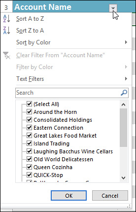
There are two basic techniques you can use in a Filter list:
Deselect an item’s check box to hide that item in the table.
Deselect the Select All item, which deselects all the check boxes, and then select the check box for each item you want to see in the table.
Using complex criteria to filter a table
The Filter command should take care of most of your filtering needs, but it’s not designed for heavy-duty work. For example, it can’t handle the following accounts receivable criteria:
Invoice amounts greater than $100, less than $1,000, or greater than $10,000
Account numbers that begin with 01, 05, or 12
Days overdue greater than the value in cell J1
To work with these more sophisticated requests, you need to use complex criteria.
Setting up a criteria range
Before you can work with complex criteria, you must set up a criteria range. A criteria range has some or all of the table field names in the top row, with at least one blank row directly underneath. You enter your criteria in the blank row below the appropriate field name, and Excel searches the table for records with field values that satisfy the criteria. This setup gives you two major advantages over the Filter command:
By using either multiple rows or multiple columns for a single field, you can create compound criteria with as many terms as you like.
Because you’re entering your criteria in cells, you can use formulas to create computed criteria.
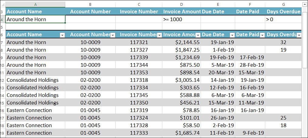
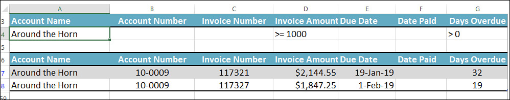
You can place the criteria range anywhere on the worksheet outside the table range. The most common position, however, is a couple of rows above the table range. Figure 17-4 shows the accounts receivable table with a criteria range (A3:G4). As you can see, the criteria are entered in the cell below the field name. In this case, the displayed criteria will find all Around the Horn invoices that are greater than or equal to $1,000 and that are overdue (that is, invoices that have a value greater than 0 in the Days Overdue field).
Filtering a table with a criteria range
After you’ve set up your criteria range, you can use it to filter the table. The following steps take you through the basic procedure:
Copy the table field names that you want to use for the criteria, and paste them into the first row of the criteria range. If you’ll be using different fields for different criteria, consider copying all your field names into the first row of the criteria range.
 Tip
TipThe only problem with copying the field names to the criteria range is that if you change a field name, you must change it in two places (that is, in the table and in the criteria). So, instead of just copying the names, you can make the field names in the criteria range dynamic by using a formula to set each criteria field name equal to its corresponding table field name. For example, you could enter =A6 in cell A3 of Figure 17-4.
Below each field name in the criteria range, enter the criteria you want to use.
Select a cell in the table and then select Data > Advanced. Excel displays the Advanced Filter dialog box, shown in Figure 17-5.
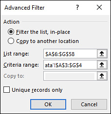
FIGURE 17-5 Use the Advanced Filter dialog box to select your table and criteria ranges. Ensure that the List Range text box contains the table range (which it should if you selected a cell in the table beforehand). If it doesn’t, select the text box and select the table (including the field names).
In the Criteria Range text box, select the criteria range (again, including the field names you copied).
To avoid including duplicate records in the filter, select the Unique Records Only check box.
Select OK. Excel filters the table to show only those records that match your criteria (see Figure 17-6).
Entering compound criteria
To enter compound criteria in a criteria range, use the following guidelines:
To find records that match all the criteria, enter the criteria on a single row.
To find records that match one or more of the criteria, enter the criteria on separate rows.
Finding records that match all the criteria is equivalent to activating the And button in the Custom AutoFilter dialog box. The sample criteria shown in Figure 17-6 match records with the account name Around the Horn and an invoice amount greater than $1,000 and a positive number in the Days Overdue field. To narrow the displayed records, you can enter criteria for as many fields as you like.
![]() Tip
Tip
You can use the same field name more than once in compound criteria. To do this, you include the appropriate field multiple times in the criteria range and enter the appropriate criteria below each label.
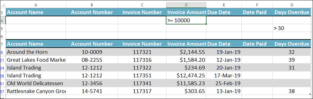
Finding records that match at least one of several criteria is equivalent to activating the Or button in the Custom AutoFilter dialog box. In this case, you need to enter each criterion on a separate row. For example, to display all invoices with amounts greater than or equal to $10,000 or that are more than 30 days overdue, you would set up your criteria as shown in Figure 17-7.
![]() Caution
Caution
Don’t include any blank rows in your criteria range because blank rows throw off Excel when it tries to match the criteria.
Entering computed criteria
The fields in your criteria range aren’t restricted to the table fields. You can create computed criteria that use a calculation to match records in the table. The calculation can refer to one or more table fields, or even to cells outside the table, and must return either TRUE or FALSE. Excel selects records that return TRUE.
To use computed criteria, add a column to the criteria range and enter the formula in the new field. Make sure that the name you give the criteria field is different from any field name in the table (or leave the name blank). When referencing the table cells in the formula, use the first data row of the table. For example, to select all records in which Date Paid is equal to Due Date in the accounts receivable table, enter the following formula:
=F6=E6
Note the use of relative addressing. If you want to reference cells outside the table, use absolute addressing.
![]() Tip
Tip
Use Excel’s AND, OR, and NOT functions to create compound computed criteria. For example, to select all records in which the Days Overdue value is less than 90 and greater than 31, type this:
=AND(G6<90, G6>31)
Figure 17-8 shows a more complex example. The goal is to select all records whose invoices were paid after the due date. The new criterion—named Late Payers—contains the following formula:
=IF(ISBLANK(F7), FALSE(), F7 > E7)
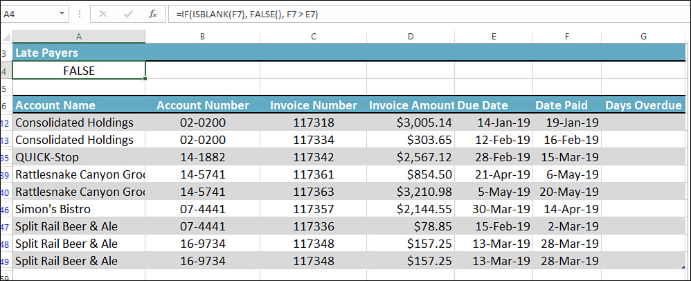
If the Date Paid field (column F) is blank, the invoice hasn’t been paid, so the formula returns FALSE. Otherwise, the logical expression F7 > E7 is evaluated. If the Date Paid field (column F) is greater than the Due Date field (column E), the expression returns TRUE, and Excel selects the record. In Figure 17-8, the Late Payers cell (A4) displays FALSE because the formula evaluates to FALSE for the first row in the table.
Filtering table data with the FILTER() function
Rather than filtering a table in-place, you might prefer to extract a filtered subset of a table and store that subset in a dynamic array. You can do that using Excel 2019’s new FILTER() function:
FILTER(array, include[, if_empty])
array |
The range, array, or table data to extract into the dynamic array. |
include |
A comparison array that determines which elements of array are included in the filtered results. |
if_empty |
The value you want Excel to return if the filter matches no values (that is, returns an empty result). |
For example, suppose you want to extract the first four columns in the table shown in Figure 17-2 and you want to filter the resulting array to include only those DVDs where the Year value is greater than or equal to 1980. Here’s a FILTER() formula that does this:
=FILTER(A2:E16, B2:B16 >= 1980)
UNIQUE()
To filter a table to return only its unique values into a dynamic array, give Excel 2019’s new UNIQUE() function a whirl:
UNIQUE(array [, by_col][, occurs_once])
array |
The range, array, or table data to extract into the dynamic array. |
by_col |
A Boolean value that specifies the filter direction: FALSE to filter by row (this is the default) or TRUE to filter by column. |
occurs_once |
A Boolean value that determines how Excel returns unique values. The default is FALSE, which means that Excel includes all unique values; to include unique values only if they occur once, use TRUE. |
For example, suppose you want to extract the unique director names in the table shown in Figure 17-2. Here’s a UNIQUE() formula that does this:
=UNIQUE(C2:C16)
Referencing tables in formulas
Excel supports a feature called structured referencing of tables. This means that Excel offers a set of defined names—or specifiers, as Microsoft calls them—for various table elements (such as the data, the headers, and the entire table), as well as the automatic creation of names for the table fields. You can include these names in your table formulas to make your calculations much easier to read and maintain.
Using table specifiers
First, let’s look at the predefined specifiers that Excel offers for tables. Table 17-1 lists the names you can use.
TABLE 17-1 Excel’s predefined table specifiers
Specifier |
Refers To |
|
The entire table, including the column headers and total row. |
|
The table data (that is, the entire table, not including the column headers and total row). |
|
The table’s column headers. |
|
The table’s total row. |
|
The table row in which the formula appears. (This was |
Most table references start with the table name (as given by the Design, Table Name property). In the simplest case, you can use the table name by itself. For example, the following formula counts the numeric values in a table named Table1:
=COUNT(Table1)
If you want to reference a specific part of the table, you must enclose that reference in square brackets after the table name. For example, the following formula calculates the maximum data value in a table named Sales:
=MAX(Sales[#Data])
![]() Tip
Tip
You can also reference tables in other workbooks by using the following syntax:
'Workbook'!Table
Here, replace Workbook with the workbook file name, and replace Table with the table name.
![]() Note
Note
Using just the table name by itself is equivalent to using the #Data specifier. So, for example, the following two formulas produce the same result:
=MAX(Sales[#Data])
=MAX(Sales)
Excel also generates column specifiers based on the text in the column headers. Each column specifier references the data in the column, so it doesn’t include the column’s header or total. For example, suppose you have a table named Inventory, and you want to calculate the sum of the values in the field named Qty On Hand. The following formula does the trick:
=SUM(Inventory[Qty On Hand])
If you want to refer to a single value in a table field, you need to specify the row you want to work with. Here’s the general syntax for this:
Table[[Row],[Field]]
Here, replace Table with the table name, Row with a row specifier, and Field with a field specifier. For the row specifier, you have only two choices: the current row and the totals row. The current row is the row in which the formula resides, and in Excel 2010 and later you use the @ specifier to designate the current row (in Excel 2007, this specifier was #This Row). In this case, however, you use @ followed by the name of the field in square brackets, like so:
@[Standard Cost]
For example, in a table named Inventory with a field named Standard Cost, the following formula multiplies the Standard Cost value in the current row by 1.25:
=Inventory[@[Standard Cost]] * 1.25
![]() Note
Note
If your formula needs to reference a cell in a row other than the current row or the totals row, you need to use a regular cell reference such as A3 or D6.
For a cell in the totals row, use the #Totals specifier, as in this example, which references the totals row for both the Qty On Hand field and the Qty On Hold field:
=Inventory[[#Totals],[Qty On Hand]] - Inventory[[#Totals],[Qty On Hold]]
Finally, you can also create ranges by using structured table referencing. As with regular cell references, you create a range by inserting a colon between two specifiers. For example, the following reference includes all the data cells in the Inventory table’s Qty On Hold and Qty On Hand fields:
Inventory[[Qty On Hold]:[Qty On Hand]]
Entering table formulas
When you build a formula using structured referencing, Excel offers several tools that make it easy and accurate. First, note that table names are part of Excel’s Formula AutoComplete feature. This means that after you type the first few letters of the table name, you’ll see the formula name in the AutoComplete list, so you can then select the name and press Tab to add it to your formula. When you then type the opening square bracket ([), Excel displays a list of the table’s available specifiers, as shown in Figure 17-9. The first few items are the field names, and the bottom four are the built-in specifiers. Select the specifier and press Tab to add it to your formula. Each time you type an opening square bracket, Excel displays the specifier list.

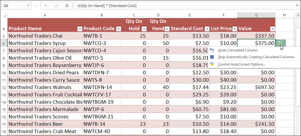
One of my favorite Excel features is its support for automatic calculated columns. To demonstrate how this works, Figure 17-10 shows a full formula that I’ve typed into a table cell but haven’t yet completed (by, say, pressing Enter). When I press Enter, Excel automatically fills the same formula into the rest of the table’s rows, as you can see in Figure 17-11. Excel also displays an AutoCorrect Options button, which enables you to reverse the calculated column, if desired.

![]() Note
Note
In Figure 17-11, notice also that Excel simplified the table formula by removing the table names, which it considers redundant.
Excel’s table functions
To take your table analysis to a higher level, you can use Excel’s table functions, which give you the following advantages:
You can enter the functions into any cell in the worksheet.
You can specify the range the function uses to perform its calculations.
You can reference a criteria range to perform calculations on subsets of the table.
About table functions
To illustrate the table functions, consider an example: If you want to calculate the sum of a table field, you can enter SUM(range), and Excel produces the result. If you want to sum only a subset of the field, you must specify as arguments the particular cells to use. For tables containing hundreds of records, however, this process is impractical.
The solution is to use DSUM(), which is the table equivalent of the SUM() function. The DSUM() function takes three arguments: a table range, field name, and criteria range. DSUM() looks at the specified field in the table and sums only records that match the criteria in the criteria range.
These functions take a little longer to set up, but the advantage is that you can enter compound and computed criteria. All these functions have the following general syntax:
Dfunction(database, field, criteria)
Dfunction |
The function name, such as DSUM or DAVERAGE. |
database |
The range of cells that make up the table you want to work with. You can use either a range name, if one is defined, or the range address. |
field |
The name of the field on which you want to perform the operation. You can use either the field name or the field number as the argument (in which the leftmost field is field number 1, the next field is field number 2, and so on). If you use the field name, enclose it in quotation marks (for example, "Total Cost"). |
criteria |
The range of cells that hold the criteria you want to work with. You can use either a range name, if one is defined, or the range address. |
![]() Tip
Tip
To perform an operation on every record in a table, leave all the criteria fields blank. This causes Excel to select every record in the table.
![]() Note
Note
If you don’t want to set up a separate criteria range, you can still analyze your tables with calculations such as counts, averages, and sums using Excel’s criteria-based worksheet functions, including COUNTIF(), AVERAGEIF(), and SUMIF(). See Chapter 11, “Building descriptive statistical formulas.”
Table 17-2 summarizes the table functions.
TABLE 17-2 Excel’s table functions
Function |
Description |
|
Returns the average of the matching records in a specified field |
|
Returns the count of the matching records |
|
Returns the count of the nonblank matching records |
|
Returns the value of a specified field for a single matching record |
|
Returns the maximum value of a specified field for the matching records |
|
Returns the minimum value of a specified field for the matching records |
|
Returns the product of the values of a specified field for the matching records |
|
Returns the estimated standard deviation of the values in a specified field if the matching records are a sample of the population |
|
Returns the standard deviation of the values of a specified field if the matching records are the entire population |
|
Returns the sum of the values of a specified field for the matching records |
|
Returns the estimated variance of the values of a specified field if the matching records are a sample of the population |
|
Returns the variance of the values of a specified field if the matching records are the entire population |
(To learn about statistical operations such as standard deviation and variance, see Chapter 11.)
You enter table functions the same way you enter any other Excel function. You type an equal sign (=) and then enter the function—either by itself or combined with other Excel operators in a formula. The following examples show valid table functions:
=DSUM(A6:H14, "Total Cost", A1:H3)
=DSUM(Table, "Total Cost", Criteria)
=DSUM(AR_Table, 3, Criteria)
=DSUM(2018_Sales, "Sales", A1:H13)
The next two sections provide examples of the DAVERAGE() and DGET() table functions.
Using DAVERAGE()
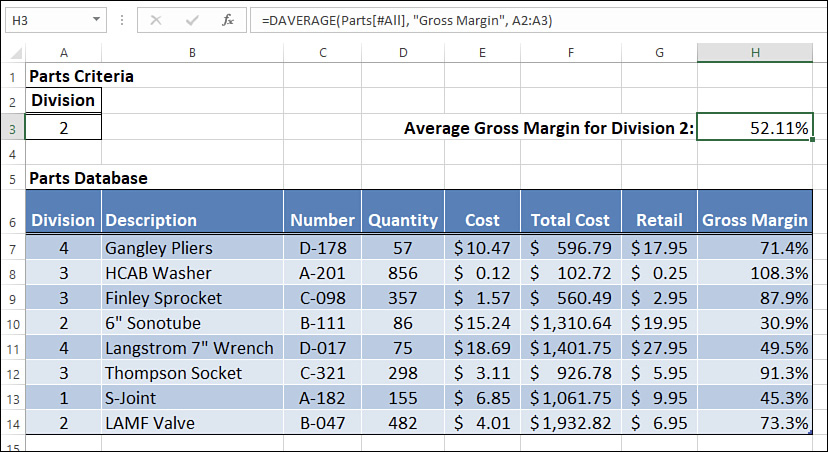
The DAVERAGE() function calculates the average field value in the database records that match the criteria. In the Parts database, for example, suppose that you want to calculate the average gross margin for all parts assigned to Division 2. You set up a criteria range for the Division field and enter 2, as shown in Figure 17-12. You then enter the following DAVERAGE() function (see cell H3):
=DAVERAGE(Parts[#All], "Gross Margin", A2:A3)
Using DGET()
The DGET() function extracts the value of a single field in the database records that match the criteria. If there are no matching records, DGET() returns #VALUE!. If there’s more than one matching record, DGET() returns #NUM!.
DGET() typically is used to query the table for a specific piece of information. For example, in the Parts table, you might want to know the cost of the Finley Sprocket. To extract this information, you would first set up a criteria range with the Description field and enter Finley Sprocket. You would then extract the information with the following formula (assuming that the table and criteria ranges are named Parts and Criteria, respectively):
=DGET(Parts[#All], "Cost", Criteria)
A more interesting application of this function would be to extract the name of a part that satisfies a certain condition. For example, you might want to know the name of the part that has the highest gross margin. Creating this model requires two steps:
Set up the criteria to match the highest value in the Gross Margin field.
Add a DGET() function to extract the description of the matching record.
Figure 17-13 shows how this is done. For the criteria, a new field called Highest Margin is created. As the text box shows, this field uses the following computed criteria:
=H7 = MAX(Parts2[Gross Margin])

Excel matches only the record that has the highest gross margin. The DGET() function in cell H3 is straightforward:
=DGET(Parts2[#All], "Description", A2:A3)
This formula returns the description of the part that has the highest gross margin.
Case study: Applying statistical table functions to a defects database
Many table functions are most often used to analyze statistical populations. Figure 17-14 shows a table of defects found among 12 work groups in a manufacturing process. In this example, the table (B3:D15) is named Defects, and two criteria ranges are used—one for each of the group leaders, Johnson (G3:G4 is Criteria1) and Perkins (H3:H4 is Criteria2).
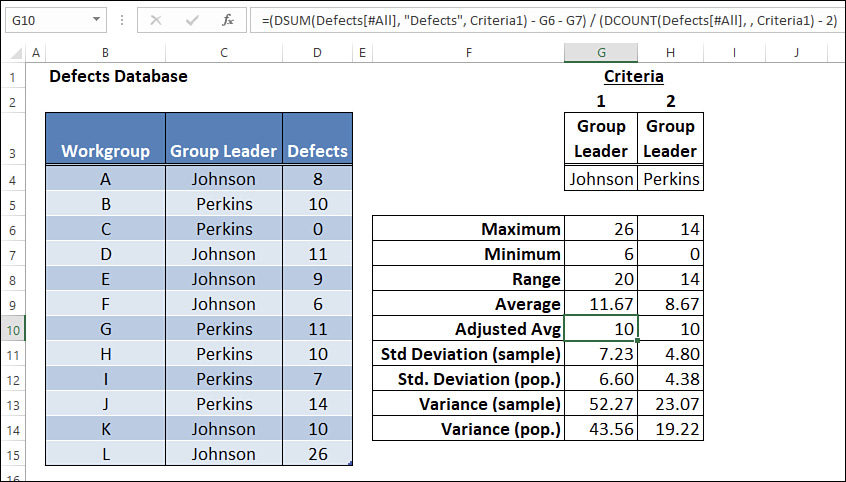
The table shows several calculations. First, DMAX() and DMIN() are calculated for each criterion. The range (a statistic that represents the difference between the largest and smallest numbers in the sample; it’s a crude measure of the sample’s variance) is then calculated using the following formula (Johnson’s groups):
=DMAX(Defects[#All], "Defects", Criteria1) - DMIN(Defects[#All], "Defects",
Criteria1)
Of course, instead of using DMAX() and DMIN() explicitly, you can simply refer to the cells containing the DMAX() and DMIN() results.
The next line uses DAVERAGE() to find the average number of defects for each group leader. Notice that the average for Johnson’s groups (11.67) is significantly higher than that for Perkins’s groups (8.67). However, Johnson’s average is skewed higher by one anomalously large number (26), and Perkins’s average is skewed lower by one anomalously small number (0).
To allow for this situation, the Adjusted Avg line uses DSUM(), DCOUNT(), and the DMAX() and DMIN() results to compute a new average without the largest and smallest number for each sample. As you can see, without the anomalies, the two leaders have the same average.
![]() Note
Note
As shown in cell G10 of Figure 17-14, if you don’t include a field argument in the DCOUNT() function, it returns the total number of records in the table.
The rest of the calculations use the DSTDEV(), DSTDEVP(), DVAR(), and DVARP() functions.