
Chapter 18
Analyzing data with PivotTables
In this chapter, you will:
Hide and customize PivotTable subtotals
Change the value field summary calculation
Create custom PivotTable calculations, including calculated fields and calculated items
Learn how to use PivotTable results in worksheet formulas
Tables and external databases can contain hundreds or even thousands of records. Analyzing that much data can be a nightmare without the right kinds of tools. To help you, Excel offers a powerful data analysis tool called a PivotTable. This tool enables you to summarize hundreds—or even hundreds of thousands—of records in a concise tabular format. You can then manipulate the layout of the table to see different views of your data. Because this is a book about Excel formulas and functions, I don’t provide instructions on building and customizing PivotTables. Instead, I focus on the extensive work you can do with built-in and custom PivotTable calculations.
Working with PivotTable subtotals
When you build a PivotTable, Excel adds grand totals for the row field and the column field. However, Excel also displays subtotals for the outer field of a PivotTable with multiple fields in the row or column area. For example, in Figure 18-1, you see two fields in the row area: Product (Mouse pad, HDMI cable, and so on) and Promotion (1 Free with 10 and Extra Discount). Product is the outer field, so Excel displays subtotals for that field.

The next few sections show you how to manipulate both the grand totals and the subtotals.
Hiding PivotTable grand totals
To remove grand totals from a PivotTable, follow these steps:
Select a cell inside the PivotTable.
Select the Design tab.
Select Grand Totals > Off for Rows and Columns. Excel removes the grand totals from the PivotTable.
Hiding PivotTable subtotals
PivotTables with multiple row or column fields display subtotals for all fields except the innermost field (that is, the field closest to the data area). To remove these subtotals, follow these steps:
Select a cell in the field.
Select the Design tab.
Select Subtotals > Do Not Show Subtotals. Excel removes the subtotals from the PivotTable.
Customizing the subtotal calculation
The subtotal calculation that Excel applies to a field is the same calculation it uses for the data area. (See the next section for details on how to change the value field summary calculation.) You can, however, change this calculation, add extra calculations, and even add a subtotal for the innermost field. Select the field you want to work with, select Analyze > Field Settings, and then use either of these methods:
To change the subtotal calculation, select Custom in the Subtotals group, select one of the calculation functions (Sum, Count, Average, and so on) in the Select One Or More Functions list, and then select OK.
To add extra subtotal calculations, select Custom in the Subtotals group, use the Select One Or More Functions list to select each calculation function you want to add, and then select OK.
Changing the value field summary calculation
By default, Excel uses a Sum function for calculating the value field summaries. Although Sum is the most common summary function used in PivotTables, it’s by no means the only one. In fact, Excel offers 11 summary functions, as outlined in Table 18-1.
TABLE 18-1 Excel’s value field summary calculations
Function |
Description |
Sum |
Adds the values for the underlying data |
Count |
Displays the total number of values in the underlying data |
Average |
Calculates the average of the values for the underlying data |
Max |
Returns the largest value for the underlying data |
Min |
Returns the smallest value for the underlying data |
Product |
Calculates the product of the values for the underlying data |
Count Numbers |
Displays the total number of numeric values in the underlying data |
StdDev |
Calculates the standard deviation of the values for the underlying data, treated as a sample |
StdDevp |
Calculates the standard deviation of the values for the underlying data, treated as a population |
Var |
Calculates the variance of the values for the underlying data, treated as a sample |
Varp |
Calculates the variance of the values for the underlying data, treated as a population |
Follow these steps to change the value field summary calculation:
Right-click any cell inside the value field.
Select Summarize Values By. Excel displays a partial list of the available summary calculations.
If you see the calculation you want, select it and skip the rest of these steps; otherwise, select More Options to open the Value Field Settings dialog box.
Select the summary calculation you want to use.
Select OK. Excel changes the value field calculation.
Using a difference summary calculation
When you analyze business data, it’s almost always useful to summarize the data as a whole: the sum of the units sold, the total number of orders, the average margin, and so on. For example, the PivotTable report shown in Figure 18-2 summarizes invoice data from a two-year period. For each customer in the row field, we see the total of all invoices broken down by the invoice date, which in this case has been grouped by year (2018 and 2019).

However, it’s also useful to compare one part of the data with another. In the PivotTable shown in Figure 18-2, for example, it would be valuable to compare each customer’s invoice totals in 2019 with those in 2018.
In Excel, you can perform this kind of analysis by using PivotTable difference calculations:
Difference From: This difference calculation compares two numeric items and calculates the difference between them.
% Difference From: This difference calculation compares two numeric items and calculates the percentage difference between them.
In each case, you must specify both a base field (the field in which you want Excel to perform the difference calculation) and the base item (the item in the base field that you want to use as the basis of the difference calculation). In the PivotTable shown in Figure 18-2, for example, Order Date would be the base field, and 2018 would be the base item.
Here are the steps to follow to set up a difference calculation:
Right-click any cell inside the value field.
Select Show Values As and then select either Difference From or % Difference From. Excel displays the Show Values As dialog box.
In the Base Field list, select the field you want to use as the base field.
In the Base Item list, select the item you want to use as the base item.
Select OK. Excel updates the PivotTable with the difference calculation.
Figure 18-3 shows both the completed Show Values As dialog box and the updated PivotTable with the Difference From calculation applied to the report from Figure 18-2.
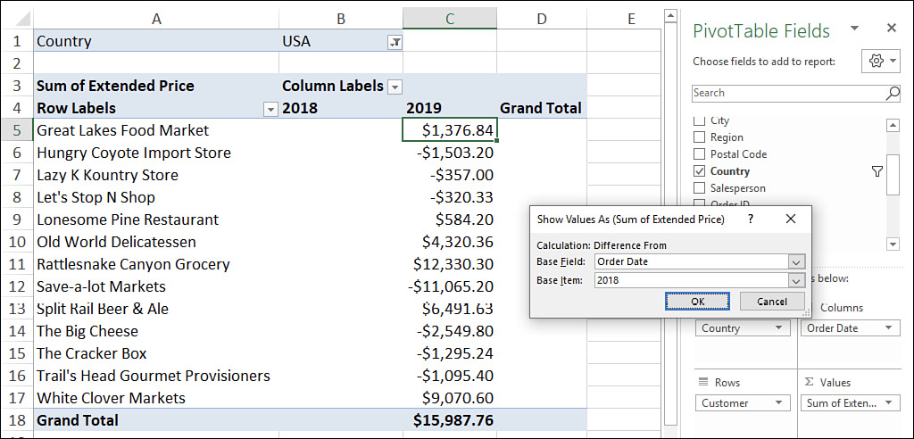
Toggling the difference calculation with VBA
Here’s a VBA macro that toggles the PivotTable report in Figure 18-3 between a Difference From calculation and a % Difference From calculation:
Sub ToggleDifferenceCalculations()
    ' Work with the first value field
    With Selection.PivotTable.DataFields(1)
        ' Is the calculation currently Difference From?
        If .Calculation = xlDifferenceFrom Then
            ' If so, change it to % Difference From
            .Calculation = xlPercentDifferenceFrom
            .BaseField = "Order Date"
            .BaseItem = "2018"
            .NumberFormat = "0.00%"
        Else
            ' If not, change it to Difference From
            .Calculation = xlDifferenceFrom
            .BaseField = "Order Date"
            .BaseItem = "2018"
            .NumberFormat = "$#,##0.00"
        End If
    End With
End Sub
Using a percentage summary calculation
When you need to compare the results that appear in a PivotTable report, just looking at the basic summary calculations isn’t always useful. For example, consider the PivotTable report in Figure 18-4, which shows the total invoices put through by various sales reps, broken down by quarter. In the fourth quarter, Margaret Peacock put through $64,429, whereas Robert King put through only $16,951. You can’t say that the first rep is (roughly) four times as good a salesperson as the second rep because their territories or customers might be completely different. A better way to analyze these numbers would be to compare the fourth quarter figures with some base value, such as the first quarter total. The numbers are down in both cases, but again the raw differences won’t tell you much. What you need to do is calculate the percentage differences and then compare them with the percentage difference in the Grand Total.
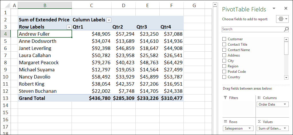
Similarly, knowing the raw invoice totals for each rep in a given quarter gives you only the most general idea of how the reps did with respect to each other. If you really want to compare them, you need to convert those totals into percentages of the quarterly grand total.
When you want to use percentages in your data analysis, you can use Excel’s percentage calculations to view data items as a percentage of some other item or as a percentage of the total in the current row, column, or the entire PivotTable. Excel offers the following percentage calculations:
% Of: This calculation returns the percentage of each value with respect to a selected base item. If you use this calculation, you must also select a base field and a base item upon which Excel will calculate the percentages.
% of Row Total: This calculation returns the percentage that each value in a row represents with respect to the Grand Total for that row.
% of Column Total: This calculation returns the percentage that each value in a column represents with respect to the Grand Total for that column.
% of Parent Row Total: If you have multiple fields in the row area, this calculation returns the percentage that each value in an inner row represents with respect to the total of the parent item in the outer row. (This calculation also returns the percentage that each value in the outer row represents with respect to the Grand Total.)
% of Parent Column Total: If you have multiple fields in the column area, this calculation returns the percentage that each value in an inner column represents with respect to the total of the parent item in the outer column. (This calculation also returns the percentage that each value in the outer column represents with respect to the Grand Total.)
% of Parent Total: If you have multiple fields in the row or column area, this calculation returns the percentage of each value with respect to a selected base field in the outer row or column. If you use this calculation, you must also select a base field upon which Excel will calculate the percentages.
% of Grand Total: This calculation returns the percentage that each value in the PivotTable represents with respect to the Grand Total of the entire PivotTable.
Here are the steps to follow to set up a difference calculation:
Right-click any cell inside the value field.
Select Show Values As and then select the percentage calculation you want to use. Excel displays the Show Values As dialog box.
If you selected either % Of or % Of Parent Total, use the Base Field list to select the field you want to use as the base field.
If you selected % Of, use the Base Item list to select the item you want to use as the base item.
Select OK. Excel updates the PivotTable with the percentage calculation.
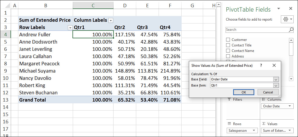
Figure 18-5 shows both the completed Show Values As dialog box and the updated PivotTable with the % Of calculation applied to the report from Figure 18-4.
![]() Tip
Tip
If you want to use a VBA macro to set the percentage calculation for a value field, set the PivotField object’s Calculation property to one of the following constants: xlPercentOf, xlPercentOfRow, xlPercentOfColumn, or xlPercentOfTotal.
When you switch back to Normal in the Show Values As list, Excel formats the value field as General, so you lose any numeric formatting you had applied. You can restore the numeric format by selecting inside the value field, choosing Analyze > Field Settings, selecting Number Format, and then choosing the format in the Format Cells dialog box. Alternatively, you can use a macro that resets the NumberFormat property. Here’s an example:
Sub ReapplyCurrencyFormat()
    With Selection.PivotTable.DataFields(1)
        .NumberFormat = "$#,##0.00"
    End With
End Sub
Using a running total summary calculation
When you set up a budget, it’s common to have sales targets not only for each month but also cumulative targets as the fiscal year progresses. For example, you might have sales targets for the first month and the second month and also for the two-month total. You’d also have cumulative targets for three months, four months, and so on. Cumulative sums such as these are known as running totals, and they can be valuable in analysis. For example, if you find that you’re running behind budget cumulatively at the six-month mark, you can make adjustments to process, marketing plans, customer incentives, and so on.
Excel PivotTable reports come with a Running Total summary calculation that you can use for this kind of analysis. Note that the running total is always applied to a base field, which is the field on which you want to base the accumulation. This is almost always a date field, but you can use other field types, as appropriate.
Here are the steps to follow to set up a running total calculation:
Right-click any cell inside the value field.
Select Show Values As > Running Total In. Excel displays the Show Values As dialog box.
Use the Base Field list to select the field you want to use as the base field.
Select OK. Excel updates the PivotTable with the running total calculation.
Figure 18-6 shows both the completed Show Values As dialog box and a PivotTable with the Running Total In calculation applied to the Order Date field (grouped by month).

![]() Tip
Tip
If you use many of these extra summary calculations, you might find yourself constantly returning the No Calculation value in the Show Values As menu. That requires a few mouse clicks, so it can be a hassle to repeat the procedure frequently. You can save time by creating a VBA macro that resets the PivotTable to Normal by setting the Calculation property to xlNoAdditionalCalculation. Here’s an example:
Sub ResetCalculationToNormal()
    With Selection.PivotTable.DataFields(1)
        .Calculation = xlNoAdditionalCalculation
    End With
End Sub
Using an index summary calculation
A PivotTable is great for reducing a large amount of relatively incomprehensible data into a compact, more easily grasped summary report. As you’ve seen in the past few sections, however, a standard summary calculation doesn’t always provide you with the best analysis of the data.
Another good example of this is trying to determine the relative importance of the results in the value field. For example, consider the PivotTable report shown in Figure 18-7. This report shows the unit sales of four items (mouse pad, HDMI cable, card reader, and USB charger), broken down by the type of advertisement the customer responded to (social media, blog network, and search).
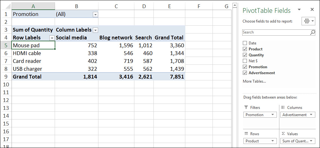
You can see, for example, that 1,012 mouse pads were sold via the search ad (the second-highest number in the report), but only 562 USB chargers were sold through the search ad (one of the lower numbers in the report). Does this mean that you should only sell mouse pads in search ads? That is, is the mouse pad/search combination somehow more “important” than the USB charger/search combination?
You might think the answer is yes to both questions in the previous paragraph, but that’s not necessarily the case. To get an accurate answer, you’d need to take into account the total number of mouse pads sold, the total number of USB chargers sold, the total number of units sold through the search ad, and the number of units overall. This is a complicated bit of business, to be sure, but each PivotTable report has an Index calculation that handles it for you automatically. The Index calculation returns the weighted average of each cell in the PivotTable value field, using the following formula:
(Cell Value * Grand Total) / (Row Total * Column Total)
In the Index calculation results, the higher the value, the more important the cell is in the overall results. Here are the steps to follow to set up an Index calculation:
Right-click any cell inside the value field.
Select Summarize Values By and then select the summary calculation you want to use.
Right-click any cell inside the value field.
Select Show Values As > Index. Excel updates the PivotTable with the index summary calculation.
Figure 18-8 shows the updated PivotTable with the Index applied to the report from Figure 18-7. As you can see, the mouse pad/search combination scored an index of only 0.90 (the second-lowest value), whereas the USB charger/search combination scored 1.17 (the highest value).

Creating custom PivotTable calculations
Excel’s 11 built-in summary functions enable you to create powerful and useful PivotTable reports, but they don’t cover every data analysis possibility. For example, suppose you have a PivotTable report that summarizes invoice totals by sales rep using the Sum function. That’s useful, but you might also want to pay out a bonus to those reps whose total sales exceed some threshold. You could use the GETPIVOTDATA() function to create regular worksheet formulas to calculate whether bonuses should be paid and how much they should be (assuming each bonus is a percentage of the total sales). (For the details on the GETPIVOTDATA() function, see “Using PivotTable results in a worksheet formula,” later in this chapter.)
However, this isn’t very convenient. If you add sales reps, you need to add formulas; if you remove sales reps, existing formulas generate errors. And, in any case, one of the points of generating a Pivot-Table report is to perform fewer worksheet calculations, not more.
The solution in this case is to take advantage of Excel’s calculated field feature. A calculated field is a new value field based on a custom formula. For example, if your invoice’s PivotTable has an Extended Price field and you want to award a 5% bonus to those reps who did at least $75,000 worth of business, you’d create a calculated field based on the following formula:
=IF('Extended Price' >= 75000, 'Extended Price' * 0.05, 0)
![]() Note
Note
When you reference a field in your formula, Excel interprets this reference as the sum of that field’s values. For example, if you include the logical expression 'Extended Price' >= 75000 in a calculated field formula, Excel interprets this as Sum of 'Extended Price' >= 75000. That is, it adds the Extended Price field and then compares it with 75000.
A slightly different PivotTable problem is when a field you’re using for the row or column labels doesn’t contain an item you need. For example, suppose your products are organized into various categories: Beverages, Condiments, Confections, Dairy Products, and so on. Suppose further that these categories are grouped into several divisions: Beverages and Condiments in Division A, Confections and Dairy Products in Division B, and so on. If the source data doesn’t have a Division field, how do you see PivotTable results that apply to the divisions?
One solution is to create groups for each division. (That is, select the categories for one division, select Analyze, Group Selection, and repeat for the other divisions.) That works, but Excel gives you a second solution: Use calculated items. A calculated item is a new item in a row or column where the item’s values are generated by a custom formula. For example, you could create a new item named Division A that is based on the following formula:
=Beverages + Condiments
Before getting to the details of creating calculated fields and items, you should know that Excel imposes a few restrictions on them. Here’s a summary:
You can’t use a cell reference, range address, or range name as an operand in a custom calculation formula.
You can’t use the PivotTable’s subtotals, row totals, column totals, or Grand Total as an operand in a custom calculation formula.
In a calculated field, Excel defaults to a Sum calculation when you reference another field in your custom formula. However, this can cause problems. For example, suppose your invoice table has Unit Price and Quantity fields. You might think that you can create a calculated field that returns the invoice totals with the following formula:
=Unit Price * Quantity
This won’t work, however, because Excel treats the Unit Price operand as Sum of Unit Price, and it doesn’t make sense to “add” the prices together.
For a calculated item, the custom formula can’t reference items from any field except the one in which the calculated item resides.
You can’t create a calculated item in a PivotTable that has at least one grouped field. You must ungroup all the PivotTable fields before you can create a calculated item.
You can’t use a calculated item as a filter.
You can’t insert a calculated item into a PivotTable in which a field has been used more than once.
You can’t insert a calculated item into a PivotTable that uses the Average, StdDev, StdDevp, Var, or Varp summary calculations.
Creating a calculated field
Here are the steps to follow to insert a calculated field into a PivotTable data area:
Select any cell in the PivotTable’s value field.
Select Analyze > Fields, Items, & Sets > Calculated Field. Excel displays the Insert Calculated Field dialog box.
Use the Name text box to enter a name for the calculated field.
Use the Formula text box to enter the formula you want to use for the calculated field.
 Note
NoteIf you need to use a field name in the formula, position the cursor where you want the field name to appear, select the field name in the Fields list, and then select Insert Field.
Select Add.
Select OK. Excel inserts the calculated field into the PivotTable.
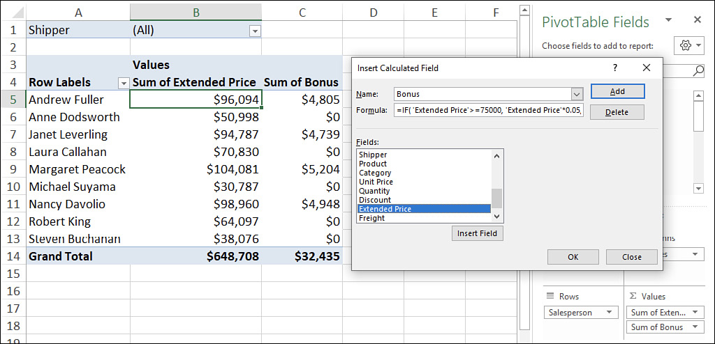
Figure 18-9 shows a completed version of the Insert Calculated Field dialog box, as well as the resulting Bonus field in the PivotTable. Here’s the full formula that appears in the Formula text box:
=IF('Extended Price' >= 75000, 'Extended Price' * 0.05, 0)
![]() Note
Note
If you need to make changes to a calculated field, select any cell in the PivotTable’s value field, select Analyze > Fields, Items, & Sets > Calculated Field, and then use the Name list to select the calculated field you want to work with. Make your changes to the formula, select Modify, and then select OK.
![]() Caution
Caution
In Figure 18-9, notice that the Grand Total row also includes a total for the Bonus field. Notice, too, that the total displayed is incorrect! This is almost always the case with calculated fields. The problem is that Excel doesn’t derive the calculated field’s Grand Total by adding up the field’s values. Instead, Excel applies the calculated field’s formula to the Grand Total of whatever field you reference in the formula. For example, in the logical expression 'Extended Price' >= 75000, Excel uses the Grand Total of the Extended Price field. Because this is definitely more than 75,000, Excel calculates the “bonus” of 5%, which is the value that appears in the Bonus field’s Grand Total.
Creating a calculated item
Here are the steps to follow to insert a calculated item into a PivotTable’s row or column area:
Select any cell in the row or column field to which you want to add the item.
Select Analyze >Fields, Items, & Sets > Calculated Item. Excel displays the Insert Calculated Item in “Field” dialog box (where Field is the name of the field you’re working with).
Use the Name text box to enter a name for the calculated item.
Use the Formula text box to enter the formula you want to use for the calculated item.
NoteTo add a field name to the formula, position the cursor where you want the field name to appear, select the field name in the Fields list, and then select Insert Field. To add a field item to the formula, position the cursor where you want the item name to appear, select the field in the Fields list, select the item in the Items list, and then select Insert Item.
Select Add.
Repeat steps 3–5 to add other calculated items to the field.
Select OK. Excel inserts the calculated item or items into the row or column field.
Figure 18-10 shows a completed version of the Insert Calculated Item in “Field” dialog box, as well as three items added to the Category row field:
Division A: =Beverage + Condiments
Division B: =Confections + 'Dairy Products'
Division C: ='Grains/Cereals' + 'Meat/Poultry' + Produce + Seafood

![]() Note
Note
To make changes to a calculated item, select any cell in the field that contains the item, select Analyze > Fields, Items, & Sets > Calculated Item, and then use the Name list to select the calculated item you want to work with. Make your changes to the formula, select Modify, and then select OK.
![]() Caution
Caution
When you insert an item into a field, Excel remembers that item. (Technically, it becomes part of the data source’s pivot cache.) If you then insert the same field into another PivotTable based on the same data source, Excel also includes the calculated items in the new PivotTable. If you don’t want the calculated items to appear in the new PivotTable report, drop down the field’s menu and deselect the check box beside each calculated item.
Using PivotTable results in a worksheet formula
What do you do when you need to include a PivotTable result in a regular worksheet formula? At first, you might be tempted just to include a reference to the appropriate cell in the PivotTable’s data area. However, that works only if your PivotTable is static and never changes. In the vast majority of cases, the reference won’t work because the addresses of the report values change as you pivot, filter, group, and refresh the PivotTable.
If you want to include a PivotTable result in a formula and you want that result to remain accurate even as you manipulate the PivotTable, use Excel’s GETPIVOTDATA() function. This function uses the value field, PivotTable location, and one or more (row or column) field/item pairs that specify the exact value you want to use. Here’s the syntax:
GETPIVOTDATA(data_field, pivot_table[, field1, item1...])
data_field |
The name of the PivotTable value field that contains the data you want |
pivot_table |
The address of any cell or range within the PivotTable, or a named range within the PivotTable |
field1 |
The name of the PivotTable row or column field that contains the data you want |
item1 |
The name of the item within field1 that specifies the data you want |
Note that you always enter the fieldn and itemn arguments as a pair. If you don’t include any field/item pairs, GETPIVOTDATA() returns the PivotTable Grand Total. You can enter up to 126 field/item pairs. This might make GETPIVOTDATA() seem like more work than it’s worth, but the good news is that you’ll rarely have to enter the GETPIVOTDATA() function by hand. By default, Excel is configured to generate the appropriate GETPIVOTDATA() syntax automatically. That is, you start your worksheet formula, and when you get to the part where you need the PivotTable value, just select the value. Excel then inserts the GETPIVOTDATA() function with the syntax that returns the value you want.
For example, in Figure 18-11, you can see that I started a worksheet formula in cell F5 by typing an equal sign (=), and then I selected cell B5 in the PivotTable. Excel generated the GETPIVOTDATA() function shown.

If Excel doesn’t generate the GETPIVOTDATA() function automatically, that feature may be turned off. Follow these steps to turn it back on:
Select File > Options to open the Excel Options dialog box.
Select Formulas.
Select the Use GetPivotData Functions For PivotTable References check box.
Select OK.
![]() Tip
Tip
You can also use a VBA procedure to toggle automatic GETPIVOTDATA() functions on and off. Set the Application.GenerateGetPivotData property to True or False, as in the following macro:
Sub ToggleGenerateGetPivotData()
    With Application
       .GenerateGetPivotData = Not .GenerateGetPivotData
    End With
End Sub