
Chapter 11
Connecting Worksheets and Workbooks
In Chapter 7, “Understanding Functions,” and Chapter 8, “Using Everyday Functions: Math, Date and Time, and Text Functions,” you find out how to set up formulas that calculate based on values within one worksheet. You can also easily connect a worksheet to several other worksheets or connect various workbooks. Excel 2019 offers easier-than-ever ways to connect a worksheet to data from the Web, data from text files, or data from databases such as Access.
In this chapter, you discover how to do the following:
Connect two worksheets
Connect two workbooks
Manage links between workbooks
Connecting Two Worksheets
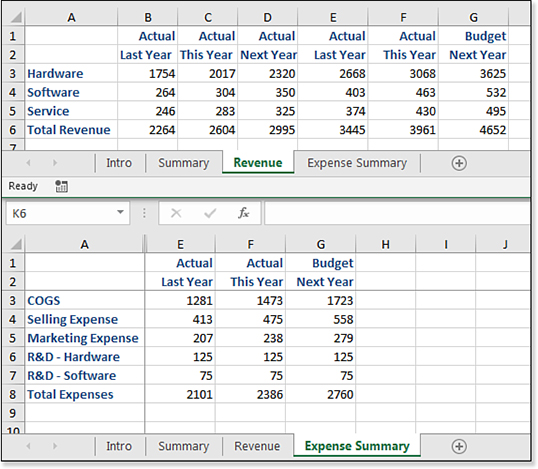
Although Excel 2019 offers 17 billion cells on every worksheet, it is fairly common to separate any model onto several worksheets. You might choose to have one worksheet for each month in a year or to have one worksheet for each functional area of a business. For example, Figure 11.1 shows a workbook with worksheets for revenue and expenses. Because different departments might be responsible for the functional areas, it makes sense to separate them into different worksheets. Eventually, though, you will want to pull information from the various worksheets into a single summary worksheet.
Excel in Practice: Seeing Two Worksheets of the Same Workbook Side by Side
The workbook in Figure 11.1 illustrates a useful trick—seeing two worksheets of the same workbook side by side. Follow these steps to see two worksheets of the same workbook side by side:
Open the first worksheet that you want to view.
On the View tab, click New Window. If your workbook is in full-screen mode, it appears that nothing happened. However, when you look in the title bar, you see your workbook title has “:2” after the title.
On the View tab, click Arrange All and then click either Vertical or Horizontal. Click the Windows of Active Workbook check box. The arrangement in Figure 11.1 is horizontal, whereas the arrangement in Figure 11.2 is vertical. Note that the Arrange All command will not work if you have any hidden workbooks open, such as the Solver add-in or a Personal Macro Workbook. In those cases, you have to resize and arrange the Excel windows manually.
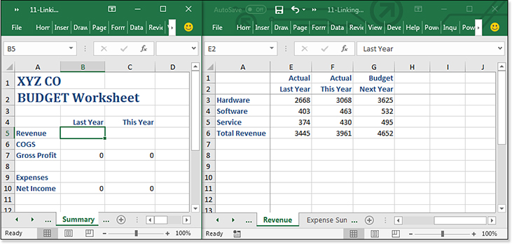
Figure 11.2 Set up a link to get information from the Revenue tab to appear on the Summary tab. In the second window, click the second worksheet tab that you want to view. You can now see both worksheets of the same workbook side by side. In Excel 2019, each window has its own ribbon and status bar.
To return to a single window, click the Close Window icon, which is the X in the top-right corner of window 2.
As shown in Figure 11.2, the goal is to have the values from cells F6:G6 on the Revenue tab carry forward to cells B5:C5 on the Summary tab. There are four ways to achieve this goal:
Type a formula, such as
=Revenue!F6, in cell B5.Build the formula using the mouse.
Right-drag cells F6:G6 on the Revenue tab to the proper location on the Summary tab and then select Link Here.
Copy cells F6:G6 on the Revenue tab. Paste to cells B5:C5 and then use the Paste Options fly-out menu to Link Here. This is the newest method and is discussed in the next section.
Note
Note that you have not created a second workbook. Instead, you have created a second camera looking at a different section of the same workbook. Any changes you make in one window appear in the other window.
Creating Links Using the Paste Options Menu
Follow these steps to set up a link using the new Paste Options fly-out menu:
Select the cells that have the figures you want to copy. For this example, select cells F6:G6 on the Revenue tab.
Press Ctrl+C to copy those cells.
Right-click the cell where the link should appear. For this example, right-click B5 on the Summary tab. In the menu that pops up, the sixth icon under Paste Options is Paste Link.
Choose Paste Link from the menu that appears (see Figure 11.3). Excel will insert formulas in B5:C5 on the Summary worksheet.
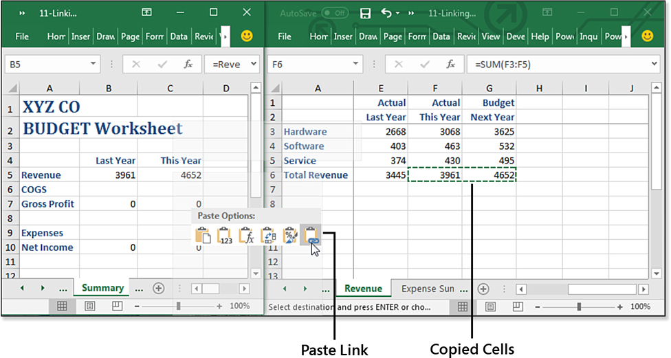
Figure 11.3 Copy the source cells to the target range.
Excel inserts a formula with the correct syntax to point to cells G6 on the Revenue tab (see Figure 11.4). Note that if data changes on the Revenue worksheet, the new results appear on the Summary worksheet.

Creating Links Using the Right-Drag Menu
If you are adept with the mouse, there is an easier way to create links. This is particularly true if you have the two worksheets arranged side by side, which was presented previously in the Excel in Practice sidebar.
This method uses the Alternate Drag-And-Drop menu. This amazing menu, which has been hiding in Excel for several versions, offers a fast way to copy cells, link cells, change formulas to values, and more.
The Alternate Drag-and-Drop menu appears anytime you right-click the border of a selection, right-drag to a new location, and then release the mouse button.
In Figure 11.5, on the Expense Summary tab, select cells F3:G3. Hover over the edge of the selection rectangle until you see the four-headed arrow. Right-click and begin to drag to the other window.

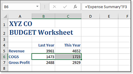
When you have arrived at the new location, release the right mouse button and select Link Here, as shown in Figure 11.6. Excel builds a formula in the target location that has the proper syntax to link to the source cells. Note that because the worksheet name contains a space, Excel wraps the sheet name in apostrophes: ='Expense Summary'!F3 (see Figure 11.7).
Building a Link by Using the Mouse
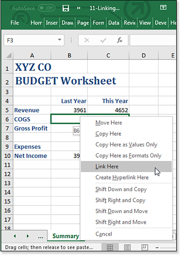
Another method is to build a formula by pointing to the correct cell with the mouse. Start in a target cell, such as cell B9 on the Summary tab (see Figure 11.8).
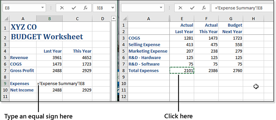
Instead of trying to remember the exact syntax, you can point to the correct cell. Type the equal sign and then click the desired worksheet tab. Using the mouse, click a cell to get the value from that cell. Excel builds the formula ='Expense Summary'!F8 in the formula bar (see Figure 11.8). Excel waits for you to either press the Enter key to accept the formula or press another operator key to add other cells to the formula.
Note
The formula that Excel builds is a relative formula. You can copy B9 to B10 to retrieve the 2018 budget.
When you press the Enter key to accept the formula, Excel jumps back to the starting worksheet. The desired figure is carried through to the worksheet.
Links to External Workbooks Default to Absolute References
You can use any of the four methods described previously for building links to other worksheets when you want to build links to external workbooks. It is easiest if you open both workbooks.
Note that if you use any of the methods illustrated previously, Excel defaults to adding dollar signs into the external reference. The dollar signs create an absolute reference that makes it more difficult to copy.
Here is an example. When you use the mouse method described in Figure 11.8 to link to a worksheet in the same workbook, the cell reference is something like F8. If you use the same method to link to a worksheet in a different workbook, the cell reference created by Excel is automatically $F$8. The dollar signs make this an absolute reference, which is difficult to copy. If you need to copy this formula to other cells, you should press the F4 key three times to change from an absolute reference to a relative reference.
Building a Formula by Typing
You can always build the links by typing the formula. This is the least popular method because you need to understand an array of syntax rules. Keep in mind that these syntax rules change depending on whether the worksheet name contains a space, whether the link is external, and whether the linked workbook is open or closed.
Here are the syntax rules:
For an internal link in which the worksheet name does not contain a space or special characters, use
=SheetName!CellAddress. An example is=Result!B3.When the worksheet name contains a space or certain special characters, Excel automatically adds apostrophes around the workbook name and sheet name. An example is
='Result Sheet'!B3.For an external link, the name of the workbook is wrapped in square brackets and appears before the sheet name. An example is
=[LinkToMe.xlsm]Sheet1!B3.If the workbook name or sheet name contains a space, add an apostrophe before the opening square bracket and after the sheet name. An example is
='[My File.xls]Income Statement'!B3.When Excel refers to a file such as [RegionTotals.xlsm], you can assume that the file is currently open. When you close the linked file, Excel updates the formula in the linking workbook to include the complete pathname. An example is
=SUM('C:[Region Totals.xlsm]Quota'!$B$2:$E$2).
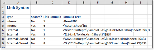
Figure 11.9 illustrates examples of various formulas.
Creating Links to Unsaved Workbooks
You can build a formula that links to a source workbook that has not been saved. This formula might point to Book1 or Book3 or the like. When you attempt to save the target workbook, Excel presents a dialog box that asks, Save <filename> with References to Unsaved Documents? In general, you should cancel the save, switch to the unsaved source workbook, and then select File, Save As to save the file with a permanent name. Then you can come back to save the linking workbook.
Using the Links Tab on the Trust Center
By default, Excel applies security settings that frustrate your attempts to pull values from closed workbooks. Consider the following scenario using two workbooks labeled Workbook A and Workbook B:
Establish a link from Workbook A to Workbook B.
Save and close Workbook A.
Make changes to Workbook B. Save and close Workbook B.
Later, open Workbook B.
Open Workbook A.
In this case, the new values in Workbook B automatically flow through to Workbook A.
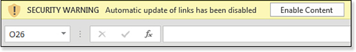
However, if you attempt to later open Workbook A before opening Workbook B, you see the following message: Automatic Update of Links Has Been Disabled (see Figure 11.10).
After you enable the content the first time, Excel marks the document as a trusted document. The next time you open the workbook, Excel displays a different cautionary message about links to external sources that could be unsafe, as shown in Figure 11.11.
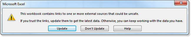
You might wonder what could be unsafe about a link. I do, too. When I asked someone at Microsoft about this, they painted an incredibly convoluted scenario that I have never seen happen. The links that are described in this section are safe. Feel free to click Update.
Opening Workbooks with Links to Closed Workbooks
Suppose that you have saved and closed the linking workbook. You update numbers in the linked workbook. You save and close the linked workbook. Later, when you open the linking workbook, Excel asks if you want to update the links to the other workbook. If you created both workbooks and you have possession of both workbooks, it is fine to allow the workbooks to update.
Dealing with Missing Linked Workbooks
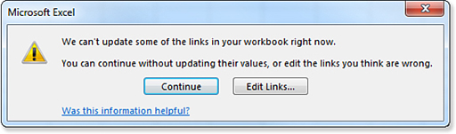
If you receive a linking workbook via email and you do not have access to the linked workbooks, Excel alerts you that the workbook contains links that cannot be updated right now. In this case, you should click Continue in the dialog box, as shown in Figure 11.12.
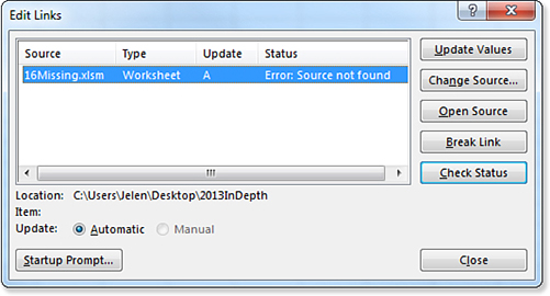
You also get this message if the linked workbook was renamed, moved, or deleted. In that case, you should click the Edit Links button to display the Edit Links dialog box (see Figure 11.13). Then you should click the Change Source button to tell Excel that the linked workbook has a new name or location. Alternatively, you might need to click the Break Link button to change all linked formulas to their current values.
Troubleshooting
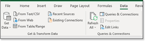
Excel warns you about links when you open the workbook and offers an Edit Links button. If you skip that box and need to Edit Links later, how do you get back to the Edit Links dialog box?
Finding the Edit Links icon does not seem logical. I am old enough to remember that it used to be on the Excel 2003 Edit menu. Now, it turns out that Edit Links is in the Queries & Connections group on the Data tab of the ribbon.
Preventing the Update Links Dialog Box from Appearing
Suppose that you need to send a linking workbook to a co-worker. You want your co-worker to see the current values of the linking formulas without having the linked workbook. In this case, you want the co-worker to click Continue in Figure 11.12. However, some newer Excel customers think that every warning box is a disaster, so you might prefer to suppress that box for your co-worker. To do so, follow these steps:
On the Data tab, in the Connections group, select Edit Links.
In the lower-left corner of the dialog box that appears, click the Startup Prompt button. The Startup Prompt dialog box appears.
Select Don’t Display The Alert And Don’t Update Automatic Links (see Figure 11.14).
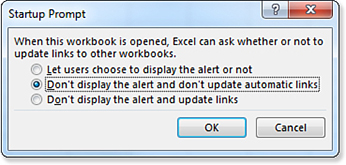
Figure 11.14 You can prevent others from seeing the Update Links message.
After emailing the workbook to your co-worker, you need to redisplay the Startup Prompt dialog box and change it back so that you will get the updated links.