Chapter 20
More Tips and Tricks for Excel 2019

The chapters in this book are full of tips and tricks. This particular chapter is a catch-all for some of the tips that did not find a home elsewhere in the book.

Watching the Results of a Distant Cell

Sometimes you need to keep an eye on a single result on a worksheet other than the one you’re currently in. For example, you might have a workbook in which assumptions on multiple worksheets produce a final ROI. As you change the assumptions, it would be good to know the effect on ROI.

It can be time consuming to constantly switch back and forth to the results worksheet after every change. Instead, you can set up a watch to show you the current value of the distant cell(s).

To set up a watch, follow these steps:

1. Select Formulas, Watch Window to display the floating Watch Window dialog box over the worksheet.

2. Click Add Watch in the Watch Window dialog box.

3. In the Add Watch dialog box, click the RefEdit button and then click the cells you want to watch.

4. Click Add to add the cell(s) to the Watch Window dialog box.

5. Repeat steps 2 through 4, as necessary.

6. Position the Watch Window dialog box in an out-of-the-way location above your worksheet so that you can continue to work.

Every time you make a change to the worksheet, the Watch Window dialog box shows you the current value of the watched cells, as shown in Figure 20.1.

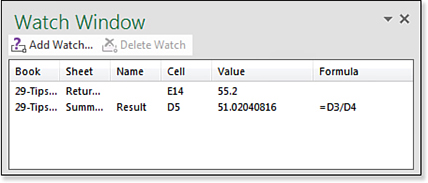
When the watch is defined, you can toggle the Watch Window dialog box by using the Watch Window icon in the Formulas tab.

Calculating a Formula in Slow Motion

If you have a particularly complicated formula, you can watch how Excel calculates the formula in slow motion. This can help you locate any logic errors in the worksheet.

To evaluate a formula in slow motion, follow these steps:

1. Select the cell that contains the formula.

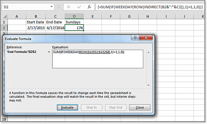
2. Select Formulas, Evaluate Formula. The Evaluate Formula dialog box appears, showing the formula. One element of the formula is underlined, indicating that this element will be calculated next.

3. To see the value of the underlined element immediately, click Evaluate.

4. If you want to see how that element is calculated, instead of clicking Evaluate, click Step In. Excel shows the formula for that element.

5. Eventually, the final level is evaluated to a number. Click Step Out to return one level up the dialog box.

6. Continue clicking Evaluate until you arrive at the answer shown in the cell.

Figure 20.2 shows an Evaluate Formula dialog box after Evaluate was clicked a few times.

Inserting a Symbol in a Cell

Obscure key combinations are available to insert many symbols. However, you do not have to learn any of them. Instead, you can use the Symbol icon on the Insert tab to display the Symbol dialog box.

In the Symbol dialog box, you scroll through many subsets of the current font. When you find the desired symbol, select it and click the Insert button.

Editing an Equation

The Equation drop-down menu on the Insert tab offers eight prebuilt equations. If you happen to need one of these equations, you can select it from the drop-down menu.

If you need to build some other equation, insert a shape in the worksheet first. While the shape is selected, use Insert, Equation, Insert New Equation. A blank equation is added to the shape.

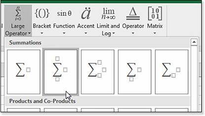
It seems very touchy, but you have to be inside the equation to have the Equation Tools Design tab showing. From the ribbon, you can open the various drop-down menus to insert a mathematical symbol. In Figure 20.3, some symbols have three placeholders. These are tiny text boxes where you can type various values.

Protecting a Worksheet

If you have many formulas in a worksheet, you might want to prevent others from changing them. In a typical scenario, your worksheet might have some input variables at the top. You might want to allow those items to be changed, but you might not want your formulas to be changed.

To protect a worksheet, follow these steps:

1. Select the input cells in your worksheet. These are the cells you want to allow someone to change.

2. Press Ctrl+1 or go to the Cells group of the Home tab and select Format, Format Cells. The Format Cells dialog box appears.

3. On the Protection tab of the Format Cells dialog box, clear the Locked check box. Click OK.

4. Select Review, Protect Sheet. The Protect Sheet dialog box appears.

5. Optionally, change what can happen in the protected workbook.

6. Click OK to apply the protection.

Repeat the Last Command with F4

Most people know that F4 is great for adding dollar signs to a reference when you are building a formula. When you are not editing a formula, the F4 key is used to repeat the previous command. Let’s say that you had to change column widths of every other column to a width of 1. After you select cell B1 and press Alt+OCW1<Enter>, you can simply press the Right Arrow key twice and press F4 to repeat the Column Width command on column D. Keep pressing Right Arrow, Right Arrow, F4 until all the column widths are fixed.

Bring the Active Cell Back in to View with Ctrl+Backspace

Sometimes, you end up at the bottom of a data set while the active cell is at the top. Press Ctrl+Backspace and Excel will scroll the active cell back into view.

Separating Text Based on a Delimiter

Depending on the source of your data, you might find that information is loaded into Excel with many fields in one cell. If the fields are separated by a character, you can separate the data into multiple columns. To do so, follow these steps:

1. Select the one-column range that contains multiple values in each cell.

2. Select Data, Data Tools, Convert Text to Column. Excel displays the Convert Text to Columns Wizard dialog box.

3. In step 1 of the wizard, select Delimited and click Next.

4. In step 2 of the wizard, choose your delimiter. Excel offers check boxes for Tab, Semicolon, Comma, and Space. If your delimiter is something different, select the Other box and type the delimiter. Click Next (see Figure 20.4).

   

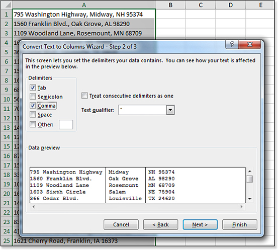
5. In step 3 of the wizard, indicate whether any of your columns are dates. Click the column in the Data Preview section and then select Date in the Column Data Format section. By default, Excel replaces the selected column and uses adjacent blank columns. To write the results to a different output area, enter a destination in step 3 of the wizard.

6. Click Finish to parse the column.

7. Excel does not automatically make the columns wide enough, so select the Cells section of the Home tab and then select Format, Width, AutoFit to make the output columns wide enough for the contents.

Auditing Worksheets Using Inquire

If you have Office 2019 Pro Plus or higher, you can enable the Inquire add-in. The add-in enables tools for discovering potential problems in workbooks. You can see a visual map of relationships, mark cells that contain certain potential problems, or compare two versions of the same workbook.

To enable Inquire, do both of these steps:

1. Press Alt+T followed by I to display the Add-Ins dialog box. Choose Inquire and click OK.

2. Select File, Options, Add-Ins. At the bottom of the screen, choose Manage Com Add-Ins and click Go. Choose Inquire and click OK. A new Inquire tab appears in the ribbon.

Suppose that you have a workbook that you send to a co-worker for review. When you receive the changed version of the workbook from the co-worker, you would like to see if any changes were made to the workbook.

Rename one or both workbooks so you can tell which is the original and which is the changed version. Open both workbooks. From the Inquire tab, choose Compare Files. Specify the newer, changed version of the workbook in the Compare drop-down menu. Specify the original workbook in the To drop-down menu. This might seem backward from the way that you would think the files should be specified.

After you click Compare, the results show in the Spreadsheet Compare tool.

If you don’t care about cell formatting changes, uncheck that category in the lower left of the window.

The top of the window shows a view of the two workbooks. Any changes are color coded to match the color legend shown in the lower left.