
Chapter 13
Transforming Data
Appending Worksheets from One Workbook
Splitting Each Delimiter to a New Row
What if there was a tool that let you clean data 20 percent faster on day one? What if that tool accurately remembered all your steps so you could clean the data 99 percent faster on days two through two hundred? That tool has been hiding on the Data tab since Excel 2016.
Power Query is the best feature to arrive in Excel about which most people have never heard. After Excel 2013 was released, the Power Query add-in was released for Excel 2010 and Excel 2013. The Add-in was great, but many people in corporate environments don’t ever see the add-ins. By the time that Excel 2016 shipped, Power Query was old news for the Excel team, and it was quietly slipped in to the Data tab of the ribbon. Unfortunately, most people never realize that the icons in the Get & Transform group are as powerful as they are.
Between Excel 2016 and Excel 2019, the tool continues to grow by leaps and bounds. You can now split by delimiter to rows, and you can combine a whole folder of Excel files.
This chapter introduces some of the tools available in Power Query as well as traditional tools such as Sort, Filter, Remove Duplicates, and Flash Fill.
Using Power Query
The Power Query tools were created to make it easier to clean ugly data. Suppose that your IT department provides a data set every day that has some problems. Rather than wait for the IT department to rewrite the query, you can use Power Query to memorize the steps needed to clean the data. When the IT department provides a new file, you simply refresh the query and Excel repeats all the data cleansing steps.
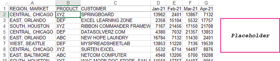
Figure 13.1 shows an ugly data set. Two different fields are in column A, separated by a comma. The customer column is in uppercase. Columns D through O are a repeating group with various month values going across. To pivot this data, you must unpivot D:O, creating an extra date column and then 12 times as many rows.
Establishing a Workflow
Say that the IT department sends you this data every month. Your plan could be to save the workbook in the same folder with the same name, and you will build your query in a new workbook. This workbook will be designed always to open the file located at C:FooUglyDataFromIT.xlsx.
Or, perhaps the file that they send each month must be combined with all of the previous monthly files. In that case, you should create a new folder to hold all of the workbooks from IT. Do not store anything else in this folder. A new workbook with the query would be saved in a different folder. In this case, you would choose Get Data, From File, From Folder.
Either of the above workflows will make it easier to refresh the query in the future. The “wrong” approach is to open the file from IT and then build the query in that file.
Loading Data Using Power Query
Power Query can load data from any of these sources:
Files: Workbook, Text, CSV, XML, JSON, or from a folder
Database: SQL Server, Access, Analysis Services, Oracle, IBM DB2, MySQL, PostgreSQL, Sybase, Teradata, and SAP HANA
Azure: SQL Database, SQL Data Warehouse, HDInsight (HDFS), Blob Storage, Table Storage, and Data Lake Store
Online: SharePoint, Exchange, Dynamics 365, Facebook, Salesforce Objects, and Salesforce Reports
Other: Table, Range, Web, Microsoft Query, SharePoint List, OData Feed, Hadoop File, ActiveDirectory, Microsoft Exchange, ODBC, and OLEDB
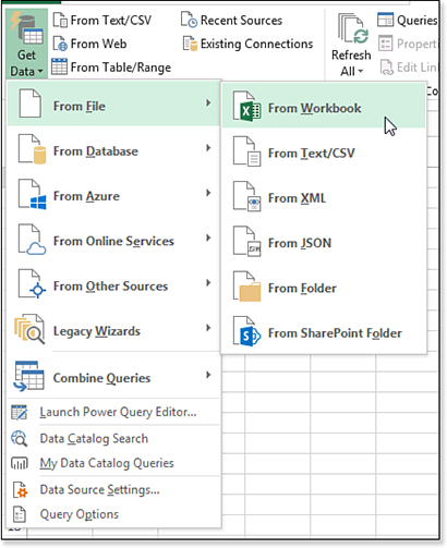
All of the preceding items are found in the Get Data menu. This is the first icon on the Data tab. It is found in the Get & Transform Data group. A few of those choices are repeated in the Get & Transform Data group: From Text/CSV, From Web, and From Table/Range.
Note
You might have previously used the legacy connectors. In previous versions of Excel, the Data tab contained seven icons: From Access, From Web, From Text, From SQL Server, From OData Data Feel, From XML Data Import, and From Data Connection Wizard. While these seven commands still exist, they have been removed from the ribbon. If you need to access the old commands, go to File, Options, Data. The Show Legacy Data Import Wizards allows you to bring the icons back. Any icons you choose here will appear under Data, Get Data, Legacy Wizards.
Loading Data from a Single Excel Workbook
Create a new blank workbook. Save the workbook with a name such as PowerQueryToLoadUglyData.xlsx.
Choose Data, Get Data, From File, From Workbook, as shown in Figure 13.2.
Depending on the source, you will need to browse to the file, provide a connect string to the database, or provide a URL.
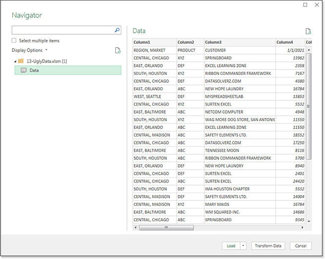
The Navigator dialog box will appear. Initially, nothing is shown in the Data Preview on the right. On the left side of the dialog box, click on the worksheet named Data. The Preview will appear on the right.
Below the Preview, you have choices to Load, Transform Data, or Cancel. You want to choose Transform Data so you can specify the data cleansing steps (see Figure 13.3).
Transforming Data in Power Query
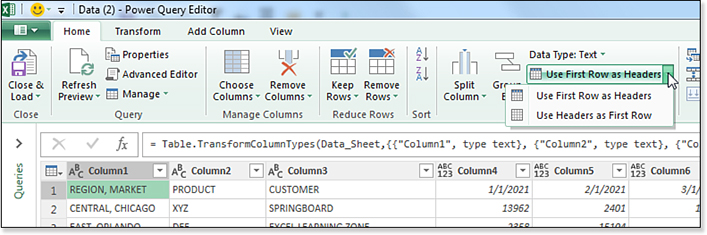
The data appears in a new window called the Query Editor. Ribbon tabs appear for Home, Transform, Add Column, and View.
As shown in Figure 13.4, Power Query is treating the header row as a data row. Use Home, Use First Row As Headers to convert that row to a header row. If you ever had the opposite problem, in which Power Query assumed the first data row is headers, you could open the same drop-down menu and choose Use Headers As First Row.
Column A has both Region and Market in a single column, separated by a comma. Select that column by clicking on the REGION, MARKET header. Use Home, Split Column, By Delimiter.
Take a look at the Split by Delimiter dialog box in Figure 13.5, which feels like the Text To Columns Wizard in Excel. However, this version is far superior.
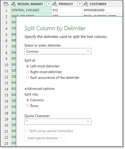
First, Power Query was able to guess that your delimiter is a comma. How did it do this? It looked at every cell in the first 20 rows and noticed a comma in each one. This is not rocket science. It makes me wonder why the Excel Text To Columns Wizard can’t figure it out.
Second, Power Query will let you split at every comma or only the first and last comma. For anyone who ever had “Mary Ellen Walton,” “Judy Norton Taylor,” or “Billy Joe Jim Bob Briggs” overwrite adjacent data after Text To Columns, you will appreciate the ability to force the results into two columns.
Finally, Power Query offers the amazing ability to split each delimiter to a new row. Data in the other columns is copied down to the new rows.
After you split a column, the new column names will be REGION, MARKET.1 and REGION, MARKET.2. Double-click each heading and type a new name such as Region for column A and Market for column B.
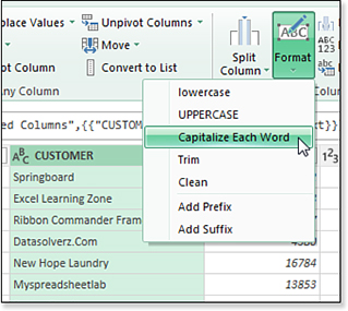
If you need to convert a column of uppercase words to proper case, select the column and select Transform, Format, Capitalize Each Word (see Figure 13.6).
Unpivoting Data in Power Query
It is very common to see data with months or years stretching across the columns. Pivot tables made from this structure are very difficult to use. In the past, fixing the data structure involved repeatedly copying and pasting, or using an obscure trick with Multiple Consolidation Ranges. Power Query makes this process amazingly simple.
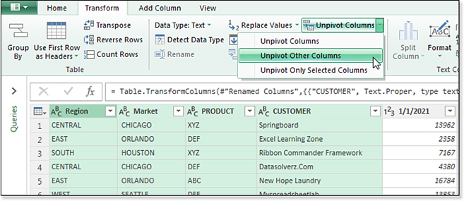
In Figure 13.7, the first four columns are selected. Use Transform, Unpivot Columns, Unpivot Other Columns.
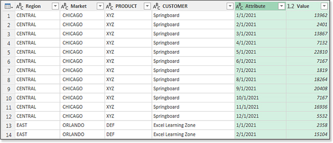
In this example, you go from 81 rows of 16 columns to 972 rows of six columns. As you can see in Figure 13.8, the fifth column is called Attribute, and the sixth column is called Value. You can use the Rename function to give these meaningful names, such as Month and Value or Month and Revenue.
Select the Date column. Look at the Data Type value on the Transform tab. Power Query is treating these dates like text. With the Date column selected, choose Date from the Data Type drop-down menu.
If there are customers who had no revenue in a certain month, you could open the Filter drop-down menu on the Value column and uncheck 0 values to remove those records.
Adding Columns in Power Query
The new Column From Examples feature in Power Query for Excel 2019 is a nice improvement. Back in Excel 2016, you would have to write a new formula to create a column. The formula language is not like the Excel language. The formula to get a month name from a date is Date.MonthName([Date]). Power Query would not accept date.monthname or Date.Monthname. You had to type Date.MonthName with the three capital letters.
Every time that I had to create a formula in Power Query, I was always going out to the web to the Power Query Function Reference.
Today, the new Column From Examples features simplifies the process (see Figure 13.9). Follow these steps:
Select the Date column.
In Power Query, choose Add Column, Column From Examples. A new Column1 appears on the far-right side of the window.
Click the first cell of Column1 and type
January.Power Query will offer a choice of Month Name from Date. Click OK.
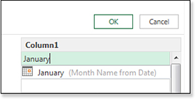
Figure 13.9 Add a new column to the query by typing an example.
Power Query will add a new column called Month Name. The Formula bar shows the formula that you would use if you plan on learning Power Query formulas.
Reviewing the Query
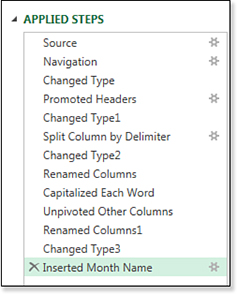
As shown in Figure 13.10, the right side of the Query Editor shows all the transformation steps that you’ve taken so far. You can see any settings associated with a step by clicking the gear icon. You can see the data at any point in the process by clicking the step. You can delete a step by using the X icon to the left of any step.
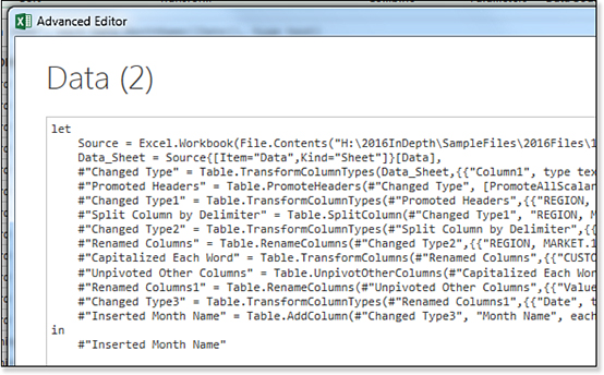
Power Query is writing an entire program in the M language behind the scenes. Go to View, Advanced Editor to see the M that was generated as you performed the data cleansing steps. Figure 13.11 shows an example.
Loading and Refreshing the Data
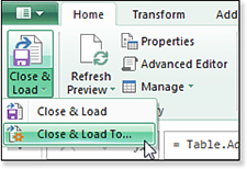
After doing all the steps to clean the data, you can choose Home, Close & Load, as shown in Figure 13.12. You can either load to an Excel worksheet or directly to the Data Model. Obviously, if you are loading more than 1,048,576 records, you will want to load the data to the Data Model.
Here is the beautiful feature: After you load the data to Excel, you can use Data, Refresh All to have the query go back to the data source, load the current data, and perform all the data cleansing steps automatically.
This is one example of the transformations available in Power Query. There is more functionality, and new functions are added monthly. You can use Power Query to consolidate all worksheets from a single file or one worksheet from multiple files.
Appending Worksheets from One Workbook
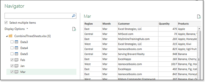
What if you have a workbook with monthly worksheets and you need to combine those records? In the Navigator dialog box, choose Select Multiple Items. Select each of the worksheet names, as shown in Figure 13.13.
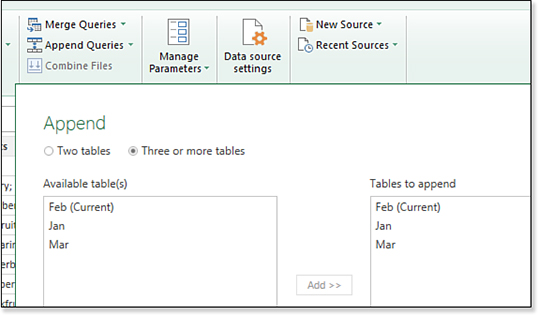
When you click Transform Data, the Power Query editor opens showing the first of several queries. On the Home tab, choose Append Queries. In the Append dialog box, choose Three Or More Tables and then move all the tables to the box on the right (see Figure 13.14).
The result will be a single query with records from all of the worksheets.
Splitting Each Delimiter to a New Row
Look at the second row of Figure 13.15. MyOnlineTrainingHub.com ordered 637 bundles of Apple; Cherry; Iceberg. You need to split those products to three rows. The customer name and all other information should be copied to the new rows.
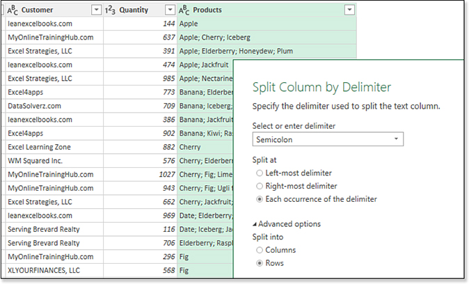
Select the Product column. Select Split Column, By Delimiter. Power Query displays the Split Column By Delimiter dialog box and correctly guesses the delimiter is a semi-colon.
Click the Advanced Options, and you will see an option to Split Into either columns or rows; choose Rows.
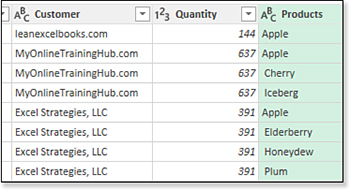
When you click OK to complete the split, the 126 rows transforms into 367 rows. Look how the 637 items for MyOnlineTrainingHub.com now appears on three separate rows in Figure 13.16.
Appending One Worksheet from Every Workbook in a Folder
While combining sheets from one workbook works, as described in the previous section, it will become unwieldy. You will have to re-create the query each month as new sheets are added. Power Query’s best trick is to combine all of the single-sheet workbooks from a single folder.
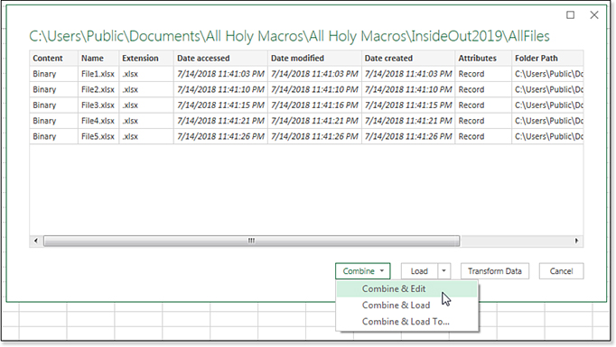
From Excel, choose Get Data, From File, From Folder, then specify the folder. Power Query will show you a list of files in the folder. Choose Combine & Edit, as shown in Figure 13.17. In the Navigator screen, choose the correct worksheet.
Power Query is smart enough to promote the first row of the first file as headers. It will then discard all of the other headers in the remaining workbooks.
If you have extra columns in some files, those columns will appear in the final query, with the word “null” for the records that did not have the extra column.
Over time, if more workbooks are added to the folder, you simply have to click Refresh to have Excel reload everything from the folder.
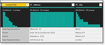
There are 91 valid values in the column.
There are 12 distinct values.
Two values occur exactly once in the column. Power Query calls these “Unique Values,” even though this seems misleading.
A chart at the top of the column indicates a histogram of the 12 unique values.
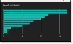
A chart at the bottom right indicates the length of the text entries.
Cleaning Data with Flash Fill
Suppose that you have data with first names in column A and last names in column B. The names are in uppercase. You would like to reshape the data, so you have the full names in proper case.
Add a heading in column C. Type the first and last name from A2 and B2 in cell C2. As soon as you type the first letter in the second cell, Excel springs into action and offers to fill the rest of the column for you (see Figure 13.18). Provided the preview looks right or even close, press Enter.
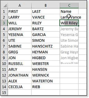
W in C3 and Excel offers to fill in the rest of the column.In addition to filling the column, Excel provides two pieces of feedback. First, the status bar in the lower-left corner of the screen indicates that Flash Fill changed a certain number of cells.
Second, a tiny on-grid Flash Fill drop-down menu icon appears next to the first changed cell. The drop-down menu offers choices such as Undo and Accept. You can also choose to select all changed cells or all unchanged cells.
Coaching Flash Fill with a Second Example
After Flash Fill operates, look for any cells that don’t fit the pattern. You might have a person with two first names (Mary Ellen Walton) or no last name (Pele). Type a new value in column C, and Flash Fill looks for other cells that match that pattern, correcting as it goes.
Flash Fill Will Not Automatically Fill in Numbers
With only 10 digits (in contrast to 26 letters), it is too likely that Excel could detect other patterns that are not the pattern you are intending. When Flash Fill sees a potential pattern, it temporarily “grays in” the suggestion but then removes the suggestion. Press Ctrl+E or click the Flash Fill icon on the Data tab to allow Flash Fill to work.
Flash Fill does not understand mathematical transformations. If the original number is 477 and you type 479 (add 2 to each cell) or 500 (round to the nearest hundred), Excel does not know how to Flash Fill the remaining cells.
Using Formatting with Dates
Dates are particularly troublesome. Suppose that you have a date of birth in column E with the format of YYYYMMDD. If you type 3/5/1970 in G2 and then press the Flash Fill icon, Excel does not correctly recognize the pattern. You get 3/5/ and the first four digits from E in each row, which is an interesting result. You can sort of understand how Excel was tricked into seeing the wrong pattern.
You can solve the date problem by formatting the column to show MM/DD/YYYY first.
Troubleshooting Flash Fill
The following are some tips for making Flash Fill work correctly:
There can be no blank columns. It is not necessary to be in the column immediately to the right of the data, but you can’t have any completely blank columns between where you want to Flash Fill and the source data.
For the automatic Flash Fill to work, you should type the first value and then immediately type the second value. Do not perform any other commands between the first and second values. Don’t type
G2, go to Sheet 3, and then come back and typeG3. By then, Flash Fill has stopped watching for patterns. The only exception is sorting. You could typeG2, sort, typeG3, and Flash Fill will work.Type a heading in the column that you are filling to prevent Flash Fill from filling your heading. Also, you could use bold for the other headings. Flash Fill follows the same rules that the Sort dialog box and the Ctrl+T Table dialog box use to detect whether there are headings. If Ctrl+T opens with the My Data Has Headings box checked, then Flash Fill does not overwrite your headings. This matters more than you might think because the headings don’t usually follow the pattern of the data and they confuse Flash Fill if it is trying to find a pattern.
Pressing Esc makes the Flash Fill preview go away. More than once, I’ve pressed Esc by mistake and lost the Flash Fill. Don’t worry. Type the first one or two cells and then use Ctrl+E or click the Flash Fill icon on the Data tab to force Excel to run Flash Fill again.
Flash Fill looks only for patterns. Flash Fill does not understand that AZ is the abbreviation for Arizona. It does not understand that Jan 23 is another way to write 1-23. Flash Fill doesn’t have any opinions. Typing
Awesomenext to Bruce Springsteen does not cue Flash Fill that you are trying to classify musical acts.
Flash Fill provides an easy way to solve many data problems. Even in the cases where an Excel pro knows a formula that can solve the problem, it is still easier to use Flash Fill.
Troubleshooting
Flash Fill can be fooled by ambiguous examples. It has an uncanny ability to see ambiguity where you could not detect it.
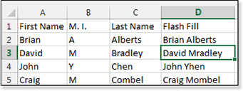
In the following example, you might type Brian Alberts in D2 and invoke Flash Fill from D3. Most rational human beings would assume that you wanted first name, a space, and last name.
Flash Fill, however, assumes that you want the first name from column A, the middle initial from column B, and then everything after the first letter of column C.
This leads to Flash Fill changing David Bradley to David Mradley. Always carefully examine the Flash Fill results to see if they make sense.
Sorting Data
Sorting in Excel 2019 is handled in the Sort dialog box or by using the AZ and ZA buttons on the Data tab. In all, there are six entry points for sorting:
Select the Home tab and then select Editing, Sort & Filter, Custom Sort.
Right-click any cell and choose Sort.
Select Sort from any filter drop-down menu.
Select the Data tab and then select Sort & Filter, AZ or Sort & Filter, ZA.
Open the Sort dialog box by going to the Data tab and selecting Sort & Filter, Sort.
The Sort dialog box in Excel 2019 offers up to 64 different sorting levels. If you get into sorting by color, you often have to specify several rules for one column, so the theoretical number of columns you can sort by is probably fewer than 64.
Sorting by Color or Icon
Excel can sort data by fill color, font color, or icon set. This also works with color applied through conditional formatting or color that you applied by using the cell format icons.
Because color is subjective, there is not a default color sequence. If one column contains 17 colors, you need to set up 17 rules in the Sort dialog box just to sort by that one column.
To sort by color, follow these steps:
Select a cell within your data.
Select the Sort icon on the Data tab. The Sort dialog box appears.
Select the desired field from the Sort By drop-down menu.
Change the Sort On drop-down menu to Cell Color.
In the Order drop-down menu, choose the color that should appear first.
In the final drop-down menu, select On Top.
To specify the next color, click the Copy Level button at the top of the Sort dialog box.
Choose the next color in the Order drop-down menu for the copied rule.
Repeat steps 7 and 8 for each additional color.
If you want to specify that values in another column should be used to break ties in the color column, select the Add Level button and specify the additional columns.
Click OK to sort the data.
Factoring Case into a Sort
Typically, an Excel sort ignores the case of the text. Values that are lowercase, uppercase, or any combination of the two are treated equally in a sort.
You can instead use a case-sensitive sort in Excel 2019 to sort lowercase values before uppercase values. For example, abc sorts before ABC. Similarly, ABc sorts before ABC.
If you want Excel to consider case when sorting, follow these steps:
Select a cell within your data.
Select the Sort icon on the Data tab. The Sort dialog box appears.
Choose the column from the Sort By drop-down menu.
Click the Options button. The Sort Options dialog box appears.
Select the Case Sensitive check box.
Click OK to close the Sort Options dialog box.
Click OK to sort.
Reordering Columns with a Left-to-Right Sort
If you receive a data set from a colleague and the columns are in the wrong sequence, you could cut and paste them into the right sequence, or you could fix them all in one pass by using a left-to-right sort. To do this, follow these steps:
Insert a new blank row above the headings.
In the new row, type numbers corresponding to the correct sequence of the columns.
Make sure that one cell in the range is selected.
Select the Sort icon on the Data tab. The Sort dialog box appears.
Click the Options button. The Sort Options dialog box appears.
Select Sort Left to Right. Click OK to close the Sort Options dialog box.
The Sort By drop-down menu now contains a list of row numbers. Choose the first row.
The remaining drop-down menus should already include Values and Smallest to Largest.
Click OK to perform the sort.
Delete your temporary extra row at the top of the data set. The columns are then resequenced into the desired order.
Tip
Excel does not change the original column widths. Select all cells with Ctrl+A and then use Home, Format, AutoFit Column Width to resize all the columns.
Sorting into a Unique Sequence by Using Custom Lists
Sometimes company tradition dictates that regions or products should be presented in an order that is not alphabetic. For example, the sequence East, Central, West makes more sense geographically than the alphabetic sequence Central, East, West.
It is possible to set up a custom list to tell Excel that the region sequence is East, Central, West. You can then sort your data based on this sequence. You need to set up the custom list only once per computer. Follow these steps to do so:
Go to a blank section of any worksheet. Type the correct sequence for the values in a column.
Select this range.
Select File, Options. The Options dialog box appears.
Click the Advanced Group. Scroll down to the General section and then select Edit Custom Lists. The Custom Lists dialog box appears.
In the Custom Lists dialog box, the bottom section shows the range of cells you selected in step 2. If it is correct, click the Import button. Your new list, with the correct sequence, is added to the default custom lists.
Click OK to close the Custom Lists dialog box. Click OK to close the Options dialog box.
Clear your temporary data range from step 1.
To use the list with custom sorting, follow these steps:
Select one cell in your data.
Select the Sort icon on the Data tab. The Sort dialog box appears.
In the Sort By drop-down menu, choose the region with the custom sort sequence.
From the Order drop-down menu, select Custom List. You should now be back in the Custom Lists dialog box.
Click your custom list and then click OK. The Sort dialog box shows that the order is based on your custom list.
Click OK to sort into the custom sequence.
One-Click Sorting
All the examples discussed so far in this chapter have used the Sort dialog box, which is required for left-to-right sorting, custom sorting, and case-sensitive sorting. It also makes color sorting easier. You can accomplish all other sorts by using the AZ buttons on the various tabs.
It is important to select a single cell in the column to be sorted. When you select a single cell, Excel extends the selection to encompass the entire current region. If you select two cells or even the whole column, Excel warns you that it is about to sort part of your data and ignore the adjacent data. This is rarely what you want.
You can find the one-click sorting options on the Home and Data tabs. On the Home tab, they are buried in the Sort & Filter drop-down menu. On the Data tab, they are clearly visible as AZ and ZA buttons.
You can also find sorting options by right-clicking a cell in the column you want to sort and selecting Sort. Options in this menu enable you to sort in ascending or descending order. You can also put the cell color, font color, or icon on top.
Additional quick-sorting options are located in the Filter drop-down menus. You can use these options to sort in ascending order, in descending order, and by color.
Fixing Sort Problems
If it appears that a sort did not work correctly, check this list of troubleshooting tips:
If the headers were sorted into the data, it usually means that one or more columns had a blank heading. Every column should have a nonblank heading. If you want the heading to appear blank, use an underscore in a white font to fool Excel. If you cannot insert a heading, you will have to use the Sort dialog box.
Unhide rows and columns before sorting. Hidden rows are not resequenced in a sort.
Use only one row for headings. If you need the headings to appear as if they are taking up several rows, put the headings in one row and wrap the text. To have control over where the text wraps, type the first line, press Alt+Enter, and then type the second line.
Data in a column should be a similar type. For example, if you have a column of ZIP Codes, you might have numeric cells for ZIP Codes of 10001 through 99999 and text cells for ZIP Codes of 00001 through 09999. This is one common way to keep leading zeroes. Because text cells are sorted sequentially after numeric cells, sorting the ZIP Codes, in this case, will appear not to work. To fix this problem, convert the entire column to one data type to achieve the expected results.
If your data has volatile formulas or formulas that point to cells outside the sort range, Excel calculates the range after sorting. If your sort sequence is based on this column, Excel accurately sorts the data, based on the information before the recalculation. If the values change after calculation, it will appear that the sort did not work.
If your data must have blank columns or rows, be sure to select the entire sort range before starting the sort process.